Excel 6 grade work book

Учебно-Методический Комплекс Excel 6

Учебно-Методический Комплекс по учебному изданию Excel 6

Содержимое разработки

УМК «EXCEL 6 FOR KAZAKHSTAN» МЕЖДУНАРОДНОГО ИЗДАТЕЛЬСТВА

A different language is a different vision of life

How many languages you know — that many times you are a person.

ОСНОВНЫЕ ЗАДАЧИ МОДЕРНИЗАЦИИ КАЗАХСТАНСКОГО ОБРАЗОВАНИЯ:

• повышение доступности, качества и эффективности образования.
• Это предполагает не только масштабные структурные, организационно-экономические изменения, но и в первую очередь — значительноеобновление содержания образования.

ОСНОВНЫЕ ПРИНЦИПЫ РАЗРАБОТКИ СИСТЕМЫ УЧЕБНИКОВ:

УМК Excel 6 for Kazakhstan:

• Индивидуальные особенности учащихся
• Подача материала с учетом этих особенностей
• Знания как средства для

• Собственная активная деятельность учащихся

ОТЛИЧИТЕЛЬНЫЕ ОСОБЕННОСТИ УМК EXCEL 6 FOR KAZAKHSTAN:

• Задания направлены на формирование и развитие коммуникативных умений в реальных ситуациях общения
• Осуществление меж предметных связей как фактора оптимизации процесса обучения английскому языку
• Проектная деятельность формирующая опыт творческой и поисковой работы

Данный курс позволяет учителю реализовать обучающий, развивающий и воспитательный потенциал каждого урока. Данный школьный возраст является благоприятным для развития творческого воображения, поэтому в учебник включены задания, способствующие приобретению детьми опыта творческой деятельности

• Знакомство с новыми словами
• Формирование предтекстовых ожиданий
• Понимание прочитанного, узнавание языковых структур
• Тренировочные и коммуникативно-ориентированные упражнения
• Песни
• Упражнения на развитие аудитивных навыков и умений

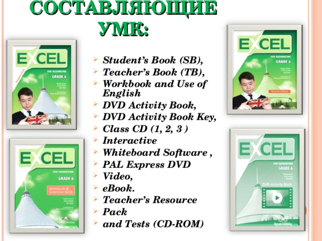
СТРУКТУРНЫЕ КОМПОНЕНТЫ СОСТАВЛЯЮЩИЕ УМК:

В УМК «Excel 6 for Kazakhstan» материал разделен на 9 тематических модулей: полностью соответствует содержанию основного общего образования по английскому языку: предметное содержание речи, коммуникативные умения по видам речевой деятельности, языковые средства и навыки пользования ими.

• Our class
• Helping&Heroes
• Our countryside
• Drama&Comedy
• Our health
• Travel&Holidays
• Reading for Pleasure
• Our neighbourhood
• Transport

Источник

EXCEL lessons for 6th grade

Articles similaires

Documents similaires

EXCEL lessons for accountants

Microsoft EXCEL lessons for high school

Microsoft EXCEL lessons for beginners

Spreadsheets EXCEL lessons intermediate

Lessons to start and advance with the python programming language from A to Z

Learn EXCEL macros and VBA step by step

Excel Cours en ligne

EXCEL course learning outcomes

Learn EXCEL for financial analysis

MS EXCEL advanced tutorial

Cours Excel 2010 Complet

Cours sur les fonctionnalités de base d Excel

Aptech Corporate Training

Corporate Office: Aptech House, A-65, MIDC, Marol, Andheri (E), Mumbai 400 093

Singrauli Network: College Road,belaunji,Waidhan, Singrauli (MP) 486 886

Tel: 07805-233001 / 09425176949 / 09770741190 E-Mail:

TABLE OF CONTENTS

Microsoft Office Button

Quick Access Toolbar

Create a Workbook

Save a Workbook

Open a Workbook Entering Data

Insert Cells, Rows and Columns

Delete Cells, Rows and Columns

Find and Replace

Calculate with Functions

Relative, Absolute, & Mixed Functions

Adding a Picture

Adding Clip Art

Editing Pictures and Clip Art

Copy a Chart to Word

Convert Text to Columns

Format Cells Dialog Box

Add Borders and Colors to Cells Change Column Width and Row Height

Hide or Unhide Rows and Columns

Align Cell Contents

Format Worksheet Tabs

Reposition Worksheets in a Workbook

Insert and Delete Worksheets

Copy and Paste Worksheets

Set Print Titles

Create a Header and a Footer

Set Page Margins

Change Page Orientation

Set Page Breaks

Split a Worksheet

Freeze and Unfreeze Rows & Columns

Hide and Unhide Worksheets

Date and time functions

Math and trigonometry functions

Lookup and reference functions

Some advance tools in excel

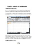
?Getting Started

Getting started with Excel 2007 you will notice that there are many similar features to previous versions. You will also notice that there are many new features that you’ll be able to utilize. There are three features that you should remember as you work within Excel 2007: the Microsoft Office Button, the Quick Access Toolbar, and the Ribbon. The function of these features will be more fully explored below.

Spreadsheets

A spreadsheet is an electronic document that stores various types of data. There are vertical columns and horizontal rows. A cell is where the column and row intersect. A cell can contain data and can be used in calculations of data within the spreadsheet. An Excel spreadsheet can contain workbooks and worksheets. The workbook is the holder for related worksheets.

Microsoft Office Button

The Microsoft Office Button performs many of the functions that were located in the File menu of older versions of Excel. This button allows you to create a new workbook, Open an existing workbook, save and save as, print, send, or close.

Ribbon

The ribbon is the panel at the top portion of the document It has seven tabs: Home, Insert, Page Layouts, Formulas, Data, Review, and View. Each tab is divided into groups. The groups are logical collections of features designed to perform function that you will utilize in developing or editing your Excel spreadsheets.

Commonly utilized features are displayed on the Ribbon. To view additional features within each group, click the arrow at the bottom right corner of each group.

: Clipboard, Fonts, Alignment, Number, Styles, Cells, Editing

: Tables, Illustrations, Charts, Links, Text

: Themes, Page Setup, Scale to Fit, Sheet Options, Arrange

: Function Library, Defined Names, Formula Auditing, Calculation

: Get External Data, Connections, Sort & Filter, Data Tools, Outline

: Proofing, Comments, Changes

: Workbook Views, Show/Hide, Zoom, Window, Macros

The quick access toolbar is a customizable toolbar that contains commands that you may want to use. You can place the quick access toolbar above or below the ribbon. To change the location of the quick access toolbar, click on the arrow at the end of the toolbar and click Show Below the Ribbon.

You can also add items to the quick access toolbar. Right click on any item in the Office Button or the Ribbon and click Add to Quick Access Toolbar and a shortcut will be added.

A new feature in Office 2007 is the Mini Toolbar. This is a floating toolbar that is displayed when you select text or right-click text. It displays common formatting tools, such as Bold, Italics, Fonts, Font Size and Font Color.

WORKING WITH WORKBOOK

Create a Workbook

To create a new Workbook:

§ Click the Microsoft Office Toolbar

§ Choose Blank Document

If you want to create a new document from a template, explore the templates and choose one that fits your needs.

Save a Workbook

When you save a workbook, you have two choices: Save or Save As. To save a document:

§ Click the Microsoft Office Button

You may need to use the Save As feature when you need to save a workbook under a different name or to save it for earlier versions of Excel. Remember that older versions of Excel will not be able to open an Excel 2007 worksheet unless you save it as an Excel 97-2003 Format. To use the Save As feature:

§ Click the Microsoft Office Button

§ Type in the name for the Workbook

§ In the Save as Type box, choose Excel 97-2003 Workbook

Open a Workbook

To open an existing workbook:

§ Click the Microsoft Office Button

§ Browse to the workbook

§ Click the title of the workbook

Entering Data

There are different ways to enter data in Excel: in an active cell or in the formula bar. To enter data in an active cell:

§ Click in the cell where you want the data

To enter data into the formula bar

§ Click the cell where you would like the data

§ Place the cursor in the Formula Bar

§ Type in the data

? MANIPULATING DATA

Excel allows you to move, copy, and paste cells and cell content through cutting and pasting and copying and pasting.

Select Data

To select a cell or data to be copied or cut:

§ Click and drag the cursor to select many cells in a range

Select a Row or Column

To select a row or column click on the row or column header.

Copy and Paste

To copy and paste data:

§ Select the cell(s) that you wish to copy

§ On the Clipboard group of the Home tab, click Copy

§ Select the cell(s) where you would like to copy the data

§ On the Clipboard group of the Home tab, click Paste

Cut and Paste

To cut and paste data:

§ Select the cell(s) that you wish to copy

§ On the Clipboard group of the Home tab, click Cut

§ Select the cell(s) where you would like to copy the data

§ On the Clipboard group of the Home tab, click Paste

Undo and Redo

To undo or redo your most recent actions:

§ On the Quick Access Toolbar

Auto Fill

The Auto Fill feature fills cell data or series of data in a worksheet into a selected range of cells. If you want the same data copied into the other cells, you only need to complete one cell. If you want to have a series of data (for example, days of the week) fill in the first two cells in the series and then use the auto fill feature. To use the Auto Fill feature:

§ Click the Fill Handle

§ Drag the Fill Handle to complete the cells

MODIFYING A WORKSHEET

Insert Cells, Rows, and Columns

To insert cells, rows, and columns in Excel:

§ Place the cursor in the row below where you want the new row, or in the column to the left of where you want the new column

§ Click the Insert button on the Cells group of the Home tab

§ Click the appropriate choice: Cell, Row, or Column

Delete Cells, Rows and Columns To delete cells, rows, and columns:

§ Place the cursor in the cell, row, or column that you want to delete

§ Click the Delete button on the Cells group of the Home tab

§ Click the appropriate choice: Cell, Row, or Column

Find and Replace

To find data or find and replace data:

§ Click the Find & Select button on the Editing group of the Home tab

§ Choose Find or Replace

§ Complete the Find What text box

§ Click on Options for more search options

Go To Command

The Go To command takes you to a specific cell either by cell reference (the Column Letter and the Row Number) or cell name.

§ Click the Find & Select button on the Editing group of the Home tab

Spell Check

To check the spelling:

§ On the Review tab click the Spelling button

PERFORMING CALCULATIONS

A formula is a set of mathematical instructions that can be used in Excel to perform calculations. Formals are started in the formula box with an = sign.

There are many elements to and excel formula.

References : The cell or range of cells that you want to use in your calculation

Operators : Symbols (+, -, *, /, etc.) that specify the calculation to be performed

Constants : Numbers or text values that do not change

Functions : Predefined formulas in Excel

To create a basic formula in Excel:

§ Select the cell for the formula

§ Type = (the equal sign) and the formula

Calculate with Functions

A function is a built in formula in Excel. A function has a name and arguments (the mathematical function) in parentheses. Common functions in Excel:

Sum: Adds all cells in the argument

Average: Calculates the average of the cells in the argument

Min: Finds the minimum value

Max: Finds the maximum value

Count: Finds the number of cells that contain a numerical value within a range of the argument

To calculate a function:

§ Click the cell where you want the function applied

§ Click the Insert Function button

§ Choose the function

§ Complete the Number 1 box with the first cell in the range that you want calculated

§ Complete the Number 2 box with the last cell in the range that you want calculated

Function Library

The function library is a large group of functions on the Formula Tab of the Ribbon. These functions include:

: Easily calculates the sum of a range

: All recently used functions

: Accrued interest, cash flow return rates and additional financial functions

: And, If, True, False, etc.

: Text based functions

: Functions calculated on date and time

Relative, Absolute and Mixed References

Calling cells by just their column and row labels (such as «A1») is called relative referencing. When a formula contains relative referencing and it is copied from one cell to another, Excel does not create an exact copy of the formula. It will change cell addresses relative to the row and column they are moved to. For example, if a simple addition formula in cell C1 «=(A1+B1)» is copied to cell C2, the formula would change to «=(A2+B2)» to reflect the new row. To prevent this change, cells must be called by absolute referencing and this is accomplished by placing dollar signs «$» within the cell addresses in the formula. Continuing the previous example, the formula in cell C1 would read «=($A$1+$B$1)» if the value of cell C2 should be the sum of cells A1 and B1. Both the column and row of both cells are absolute and will not change when copied. Mixed referencing can also be used where only the row OR column fixed. For example, in the formula «=(A$1+$B2)», the row of cell A1 is fixed and the column of cell B2 is fixed.

Linking Worksheets

You may want to use the value from a cell in another worksheet within the same workbook in a formula. For example, the value of cell A1 in the current worksheet and cell A2 in the second worksheet can be added using the format «sheetname!celladdress». The formula for this example would be «=A1+Sheet2!A2» where the value of cell A1 in the current worksheet is added to the value of cell A2 in the worksheet named «Sheet2».

?SORT AND FILTER

Sorting and Filtering allow you to manipulate data in a worksheet based on given set of criteria.

Basic Sorts

To execute a basic descending or ascending sort based on one column:

§ Highlight the cells that will be sorted

§ Click the Sort & Filter button on the Home tab

§ Click the Sort Ascending (A-Z) button or Sort Descending (Z-A) button

Custom Sorts

To sort on the basis of more than one column:

§ Click the Sort & Filter button on the Home tab

§ Choose which column you want to sort by first

§ Click Add Level

§ Choose the next column you want to sort

Filtering

Filtering allows you to display only data that meets certain criteria. To filter:

§ Click the column or columns that contain the data you wish to filter

§ On the Home tab, click on Sort & Filter

§ Click Filter button

§ Click the Arrow at the bottom of the first cell

§ Click the Text Filter

§ Click the Words you wish to Filter

§ To clear the filter click the Sort & Filter button

?GRAPHICS

Adding a Picture To add a picture:

§ Click the Insert tab

§ Click the Picture button

§ Browse to the picture from your files

§ Click the name of the picture

§ To move the graphic, click it and drag it to where you want it

Adding Clip Art To add Clip Art:

§ Click the Insert tab

§ Click the Clip Art button

§ Search for the clip art using the search Clip Art dialog box

§ Click the clip art

§ To move the graphic, click it and drag it to where you want it

Editing Pictures and Clip Art

When you add a graphic to the worksheet, an additional tab appears on the Ribbon. The Format tab allows you to format the pictures and graphics. This tab has four groups:

Adjust: Controls the picture brightness, contrast, and colors

Picture Style: Allows you to place a frame or border around the picture and add effects

Arrange: Controls the alignment and rotation of the picture

Size: Cropping and size of graphic

Adding Shapes To add Shape:

§ Click the Insert tab

§ Click the Shapes button

§ Click the shape you choose

§ Click the Worksheet

§ Drag the cursor to expand the Shape

To format the shapes:

§ Click the Shape

§ Click the Format tab

Adding SmartArt

SmartArt is a feature in Office 2007 that allows you to choose from a variety of graphics, including flow charts, lists, cycles, and processes. To add SmartArt:

§ Click the Insert tab

§ Click the SmartArt button

§ Click the SmartArt you choose

§ Select the Smart Art

§ Drag it to the desired location in the worksheet

To format the SmartArt:

§ Select the SmartArt

§ Click either the Design or the Format tab

§ Click the SmartArt to add text and pictures.

?CHARTS

Charts allow you to present information contained in the worksheet in a graphic format. Excel offers many types of charts including: Column, Line, Pie, Bar, Area, Scatter and more. To view the charts available click the Insert Tab on the Ribbon.

Create a Chart

To create a chart:

§ Select the cells that contain the data you want to use in the chart

§ Click the Insert tab on the Ribbon

§ Click the type of Chart you want to create

Modify a Chart

Once you have created a chart you can do several things to modify the chart.

To move the chart:

§ Click the Chart and Drag it another location on the same worksheet, or

§ Click the Move Chart button on the Design tab

§ Choose the desired location (either a new sheet or a current sheet in the workbook)

To change the data included in the chart:

§ Click the Chart

§ Click the Select Data button on the Design tab

To reverse which data are displayed in the rows and columns:

§ Click the Chart

§ Click the Switch Row/Column button on the Design tab

To modify the labels and titles:

§ Click the Chart

§ On the Layout tab, click the Chart Title or the Data Labels button

§ Change the Title and click Enter

The Chart Tools appear on the Ribbon when you click on the chart. The tools are located on three tabs: Design, Layout, and Format.

Within the Design tab you can control the chart type, layout, styles, and location.

Within the Layout tab you can control inserting pictures, shapes and text boxes, labels, axes, background, and analysis.

Within the Format tab you can modify shape styles, word styles and size of the chart.

Copy a Chart to Word

§ Select the chart

§ Click Copy on the Home tab

§ Go to the Word document where you want the chart located

§ Click Paste on the Home tab

?FORMATTING A WORKSHEET

Convert Text to Columns

Sometimes you will want to split data in one cell into two or more cells. You can do this easily by utilizing the Convert Text to Columns Wizard.

§ Highlight the column in which you wish to split the data

§ Click the Text to Columns button on the Data tab

§ Click Delimited if you have a comma or tab separating the data, or click fixed widths to set the data separation at a specific size.

Modify Fonts

Modifying fonts in Excel will allow you to emphasize titles and headings. To modify a font:

§ Select the cell or cells that you would like the font applied

§ On the Font group on the Home tab, choose the font type, size, bold, italics, underline, or color

Format Cells Dialog Box

In Excel, you can also apply specific formatting to a cell. To apply formatting to a cell or group of cells:

§ Select the cell or cells that will have the formatting

§ Click the Dialog Box arrow on the Alignment group of the Home tab

There are several tabs on this dialog box that allow you to modify properties of the cell or cells.

Number : Allows for the display of different number types and decimal places

Alignment : Allows for the horizontal and vertical alignment of text, wrap text, shrink text, merge cells and the direction of the text.

Font : Allows for control of font, font style, size, color, and additional features

Border : Border styles and colors

Fill: Cell fill colors and styles

Add Borders and Colors to Cells

Borders and colors can be added to cells manually or through the use of styles. To add borders manually:

§ Click the Borders drop down menu on the Font group of the Home tab

§ Choose the appropriate border

To apply colors manually:

§ Click the Fill drop down menu on the Font group of the Home tab § Choose the appropriate color

To apply borders and colors using styles:

§ Click Cell Styles on the Home tab

§ Choose a style or click New Cell Style

Change Column Width and Row Height

To change the width of a column or the height of a row:

§ Click the Format button on the Cells group of the Home tab

§ Manually adjust the height and width by clicking Row Height or Column Width

§ To use AutoFit click AutoFit Row Height or AutoFit Column Width

Hide or Unhide Rows or Columns To hide or unhide rows or columns:

§ Select the row or column you wish to hide or unhide

§ Click the Format button on the Cells group of the Home tab

§ Click Hide & Unhide

Merge Cells

To merge cells select the cells you want to merge and click the Merge & Center button on the Alignment group of the Home tab. The four choices for merging cells are:

Merge & Center: Combines the cells and centers the contents in the new, larger cell

Merge Across: Combines the cells across columns without centering data

Merge Cells: Combines the cells in a range without centering Unmerge Cells: Splits the cell that has been merged

Align Cell Contents

To align cell contents, click the cell or cells you want to align and click on the options within the Alignment group on the Home tab. There are several options for alignment of cell contents:

: Aligns text to the top of the cell

: Aligns text between the top and bottom of the cell

: Aligns text to the bottom of the cell

Align Text Left

: Aligns text to the left of the cell

: Centers the text from left to right in the cell

Align Text Right

: Aligns text to the right of the cell

: Decreases the indent between the left border and the text

: Increase the indent between the left border and the text

: Rotate the text diagonally or vertically

?DEVELOPING A WORKBOOK

Format Worksheet Tab

You can rename a worksheet or change the color of the tabs to meet your needs. To rename a worksheet:

§ Open the sheet to be renamed

§ Click the Format button on the Home tab

§ Click Rename sheet

§ Type in a new name

To change the color of a worksheet tab:

§ Open the sheet to be renamed

§ Click the Format button on the Home tab

§ Click Tab Color

§ Click the color

Reposition Worksheets in a Workbook To move worksheets in a workbook:

§ Open the workbook that contains the sheets you want to rearrange

§ Click and hold the worksheet tab that will be moved until an arrow appears in the left corner of the sheet

§ Drag the worksheet to the desired location

Insert and Delete Worksheets

To insert a worksheet

§ Open the workbook

§ Click the Insert button on the Cells group of the Home tab

§ Click Insert Sheet

To delete a worksheet

§ Open the workbook

§ Click the Delete button on the Cells group of the Home tab

§ Click Delete Sheet

Copy and Paste Worksheets: To copy and paste a worksheet:

§ Click the tab of the worksheet to be copied

§ Right click and choose Move or Copy

§ Choose the desired position of the sheet

§ Click the check box next to Create a Copy

11 PAGE PROPERTIES AND PRINTING

Set Print Titles

The print titles allows you to repeat the column and row headings at the beginning of each new page to make reading a multiple page sheet easier to read when printed. To Print Titles:

§ Click the Page Layout tab on the Ribbon

§ Click the Print Titles button

§ In the Print Titles section, click the box to select the rows/columns to be repeated § Select the row or column

§ Click the Select Row/Column Button

To create a header or footer:

§ Click the Header & Footer button on the Insert tab

§ This will display the Header & Footer Design Tools Tab

§ To switch between the Header and Footer, click the Go to Header or Go to Footer button

§ To insert text, enter the text in the header or footer

§ To enter preprogrammed data such as page numbers, date, time, file name or sheet name, click the appropriate button

§ To change the location of data, click the desired cell

Set Page Margins

To set the page margins:

1. Click the Margins button on the Page Layout tab

2. Select one of the give choices, or

§ Click Custom Margins

§ Complete the boxes to set margins

Change Page Orientation

To change the page orientation from portrait to landscape:

§ Click the Orientation button on the Page Layout tab

§ Choose Portrait or Landscape

Set Page Breaks

You can manually set up page breaks in a worksheet for ease of reading when the sheet is printed. To set a page break:

§ Click the Breaks button on the Page Layout tab

§ Click Insert Page Break

Print a Range

There may be times when you only want to print a portion of a worksheet. This is easily done through the Print Range . To print a range:

§ Select the area to be printed

§ Click the Print Area button on the Page Layout tab

§ Click Select Print Area

Split a Worksheet

You can split a worksheet into multiple resizable panes for easier viewing of parts of a worksheet. To split a worksheet:

§ Select any cell in center of the worksheet you want to split

§ Click the Split button on the View tab

§ Notice the split in the screen, you can manipulate each part separately

Freeze Rows and Columns

You can select a particular portion of a worksheet to stay static while you work on other parts of the sheet. This is accomplished through the Freeze Rows and Columns . To Freeze a row or column:

§ Click the Freeze Panes button on the View tab

§ Either select a section to be frozen or click the defaults of top row or left column

§ To unfreeze, click the Freeze Panes button

Hide Worksheets

To hide a worksheet:

§ Select the tab of the sheet you wish to hide

§ Right-click on the tab

To unhide a worksheet:

§ Right-click on any worksheet tab

§ Choose the worksheet to unhide

Worksheet functions are categorized by their functionality. In Excel there are various categories of functions. These are:

1. Text functions

2. Date and time functions

3. Math and trigonometry functions

4. Logical functions

5. Financial functions

6. Lookup and reference functions

7. Statistical functions

Returns the character specified by the code number

Returns a numeric code for the first character in a text string

Joins several text items into one text item

Returns the leftmost characters from a text value

Returns the number of characters in a text string

Converts text to lowercase

Returns a specific number of characters from a text string starting at the position you specify

Capitalizes the first letter in each word of a text value

Returns the rightmost characters from a text value

Formats a number and converts it to text

Removes spaces from text

Converts text to uppercase

Date and time functions

Returns the serial number of a particular date

Converts a serial number to a day of the month

Calculates the number of days between two dates based on a 360-day year

Converts a serial number to an hour

Converts a serial number to a minute

Converts a serial number to a month

Returns the serial number of the current date and time

Converts a serial number to a second

Returns the serial number of a particular time

Returns the serial number of today’s date

Converts a serial number to a year

Math and trigonometry functions

Returns the absolute value of a number

Rounds a number to the nearest integer or to the nearest multiple of significance

Returns the factorial of a number

Rounds a number down, toward zero

Returns the greatest common divisor

Rounds a number down to the nearest integer

Returns the least common multiple

Returns the remainder from division

Returns the value of pi

Returns the result of a number raised to a power

Multiplies its arguments

Converts an arabic numeral to roman, as text

Rounds a number to a specified number of digits

Rounds a number down, toward zero

Rounds a number up, away from zero

Returns a positive square root

Adds its arguments

Adds the cells specified by a given criteria

Adds the cells in a range that meet multiple criteria

Returns TRUE if all of its arguments are TRUE

Returns TRUE if any argument is TRUE

Reverses the logic of its argument

Specifies a logical test to perform

Returns a value you specify if a formula evaluates to an error; otherwise, returns the result of the formula

Returns the future value of an investment

Returns the periodic payment for an annuity

Returns the payment on the principal for an investment for a given period

Lookup and reference functions

Looks in the top row of an array and returns the value of the indicated cell

Looks up values in a vector or array

Looks in the first column of an array and moves across the row to return the value of a cell

Returns the average of its arguments

Returns the average (arithmetic mean) of all the cells in a range that meet a given criteria

Returns the average (arithmetic mean) of all cells that meet multiple criteria

Counts how many numbers are in the list of arguments

Counts the number of cells within a range that meet the given criteria

Counts the number of cells within a range that meet multiple criteria

Returns the maximum value in a list of arguments

Returns the median of the given numbers

Returns the minimum value in a list of arguments

Returns a vertical array of the most frequently occurring, or repetitive values in an array or range of data

The standard deviation is a measure of how widely values are dispersed from the average value (the mean).

(1) CHAR function

Description: Returns the character specified by the code number.

Syntax: =CHAR(ASCII Code)

(2) CODE function

Description: Returns a numeric code for the first character in a text string.

Syntax: =CODE(ASCII Character)

(3) CONCATENATE function

Description: Joins several text items into one text item.

(4) LEFT function

Description: Returns the leftmost characters from a text value.

Syntax: =LEFT(text, num_chars)

(5) LEN function

Description: Returns the number of characters in a text string.

(6) LOWER function

Description: Converts text to lowercase.

(7) MID function

Description: Returns a specific number of characters from a text string starting at the position you specify.

Syntax: =MID(Text, Statr_num, Num_chars)

(8) PROPER function

Description: Capitalizes the first letter in each word of a text value.

(9) RIGHT function

Description: Returns the rightmost characters from a text value.

Syntax: =RIGHT(text, num_chars) Example:

(10) TEXT function

Description: Formats a number and converts it to text.

Syntax: =TEXT(Value,Format_text) Example:

(11) TRIM function

Description: Removes leading and trailing spaces from text.

Syntax: =TRIM(text) Example:

(12) UPPER function

Description: Converts text to uppercase.

(1) DATE function

Description: Returns the serial number of a particular date.

Syntax: =DATE(year,month,day) Example:

(2) DAY function

Description: Converts a serial number to a day of the month.

(3) DAYS360 function

Description: Calculates the number of days between two dates based on a 360-day year.

Syntax: =DAYS360(start_date ,end_date) Example:

(4) HOUR function

Description: Converts a serial number to an hour.

(5) MINUTE function

Description: Converts a serial number to a minute.

(6) MONTH function

Description: Converts a serial number to a month.

(7) NOW function

Description: Returns the serial number of the current date and time.

(8) SECOND function

Description: Converts a serial number to a second.

(9) TIME function

Description: Returns the serial number of a particular time.

Syntax: =TIME(hour, minute, second) Example:

(10) TODAY function

Description: Returns the serial number of today’s date.

(11) YEAR function

Description: Converts a serial number to a year.

(1) ABS function

Description: Returns the absolute value of a number.

(2) CEILING function

Description: Rounds a number to the nearest integer or to the nearest multiple of significance.

Syntax: =CEILING(number, significance) Example:

(3) FACT function

Description: Returns the factorial of a number.

(4) FLOOR function

Description: Rounds a number down, toward zero.

Syntax: =FLOOR(number, significance) Example:

(5) GCD function

Description: Returns the greatest common divisor.

Syntax: =GCD(number1, number2, ………..) Example:

(6) INT function

Description: Rounds a number down to the nearest integer.

(7) LCM function

Description: Returns the least common multiple.

Syntax: =LCM(number1, number2, …………) Example:

(8) MOD function

Description: Returns the remainder from division.

Syntax: =MOD(number, divisor) Example:

(9) PI function

Description: Returns the value of pi.

Syntax: =PI() Example:

(10) POWER function

Description: Returns the result of a number raised to a power.

Syntax: =POWER(number, power) Example:

(11) PRODUCT function

Description: Multiplies its arguments.

Syntax: =PRODUCT(number1, number2, …………..) Example:

(12) ROMAN function

Description: Converts an arabic numeral to roman, as text.

(13) ROUND function

Description: Rounds a number to a specified number of digits.

Syntax: =ROUND(number, num_digits) Example:

(14) ROUNDDOWN function

Description: Rounds a number down, toward zero

Syntax: =ROUNDDOWN(number, num_digits) Example:

(15) ROUNDUP function

Description: Rounds a number up, away from zero.

Syntax: =ROUNDUP(number, num_digits) Example:

(16) SQRT function

Description: Returns a positive square root.

(17) SUM function

Description: Adds its arguments.

Syntax: =SUM(number1, number2, ………….) OR SUM(range) Example:

(18) SUMIF function

Description: Adds the cells specified by a given criteria.

Syntax: =SUMIF(range, criteria, [sumrange]) Example:

(19) SUMIFS function

Description: Adds the cells in a range that meet multiple criteria.

Syntax: =SUMIFS(sum_range, criteria_range1, criteria1, criteria_range2, criteria2,……) Example:

(1) AND function

Description: Returns TRUE if all of its arguments are TRUE. Syntax: =AND(logical1, logical2, ………) Example:

(2) OR function

Description: Returns TRUE if any argument is TRUE. Syntax: =OR(logical1, logical2,…………..) Example:

(3) NOT function

Description: Reverses the logic of its argument.

Syntax: =NOT(logical) Example:

(4) IF function

Description: Specifies a logical test to perform.

Syntax: =IF(logical_test, value_if_true, value_if_false) Example:

(5) IFERROR function

Description: Returns a value you specify if a formula evaluates to an error; otherwise, returns the result of the formula.

Syntax: =IFERROR(value, value_if_error) Example:

(1) FV function

Description: Returns the future value of an investment.

=FV (rate, nper,-pmt, [pv], [type])

Required. The interest rate per period.

Required. The total number of payment periods in an annuity.

Required. The payment made each period,

Optional. The present value or the lump-sum amount that a series of future

payments is worth right now. If pv is omitted, it is assumed to be 0 (zero), and you must include the pmt argument.

Type: Optional. The number 0 or 1 and indicates when payments are due. If type is

omitted, it is assumed to be 0. Example:

(2) PMT function

Description: Returns the periodic payment for an annuity. Syntax: =PMT (rate, nper,-pmt, [pv], [type]) Example:

(1) HLOOKUP function

Description: Looks in the top row of an array and returns the value of the indicated cell. Syntax: =HLOOKUP(lookup_value, table_array, row_index_num, [range_lookup]) Example:

(2) LOOKUP function

Description: Looks up values in a vector or array.

Syntax: =LOOKUP(lookup_value, lookup_vector, [result_vector]) Example:

(3) VLOOKUP function

Description: Looks in the first column of an array and moves across the row to return the value of a cell.

Syntax: =VLOOKUP(lookup_value, table_array, col_index_num, [range_lookup]) Example:

(1) AVERAGE function

Description: Returns the average of its arguments. Syntax: =AVERAGE(number1, number2, …………………….) Example:

(2) AVERAGEIF function

Description: Returns the average (arithmetic mean) of all the cells in a range that meet a given criteria.

Syntax: =AVERAGEIF (range, criteria, average_range) Example:

(3) AVERAGEIFS function

Description: Returns the average (arithmetic mean) of all cells that meet multiple criteria.

Syntax: =AVERAGEIFS(average_range, criteria_range1, criteria1, criteria_range2, criteria2, ………..) Example:

(4) COUNT function

Description: Counts how many numbers are in the list of arguments.

Syntax: =COUNT(value1, value2, …………………) Example:

(5) COUNTIF function

Description: Counts the number of cells within a range that meet the given criteria.

Syntax: =COUNTIF(range, criteria) Example:

(6) COUNTIFS function

Description: Counts the number of cells within a range that meet multiple criteria. Syntax: =COUNTIFS(range1, criteria1, range2, criteria2, ………………) Example:

(7) MAX function

Description: Returns the maximum value in a list of arguments.

Syntax: =MAX (value1, value2, ……..)

(8) MEDIAN function

Description: Returns the median of the given numbers.

Syntax: =MEDIAN (number1, number2, ………………)

(9) MIN function

Description: Returns the minimum value in a list of arguments.

Syntax: =MIN (value1, value2, ……………..)

(10) MODE function

Description: Returns a vertical array of the most frequently occurring, or repetitive values in an array or range of data.

Syntax: =MODE (number1, number2)

(11) STDEV function

Description: The standard deviation is a measure of how widely values are dispersed from the average value (the mean).

Syntax: =STDEV (number1, number2, …………………)

DATA VALIDATION

If you want to restrict data entry on a worksheet, you can setup data validation by doing the following.

1. Select A1 cell to validate.

2. On the Data tab, in the Data Tools group, click Data Validation.

3. The Data Validation dialog box is displayed.

4. Click on Settingtab. Select Whole Number from Allow dropdown. Select Between from Data dropdown. Enter 100 on Minimum textbox and enter 200 on maximum textbox.

5. Click on Input Message tab.

6. Type ‘Enter a number’ on Input Message textbox.

7. Click on Error Alert tab.

8. Type ‘Number not valid’ on Error message textbox.

9. Click on OK button.

10. Select validated cell and enter a number less than 100.

11. You will receive a validate message.

SUBTOTAL

1. Create a worksheet and enter data as following.

2. For date wise totaling, sort Date column in ascending order.

3. Click on Data tab. Go to Outline group and select Subtotal.

4. The Subtotal dialog box is displayed.

5. Select Date from At each change in drop down. Select Sum from Select Sum from Use function drop down. Click on Diesel, Petrol, Lube checkbox from Add subtotal to checkbox list.

6. Click on OK button.

7. You will see your result as follows:

8. In left hand side there are 3 outline symbols 1,2,3,+ and -.

9. When you click on 1, your output as follows.

10. When you click on 2, your output as follows.

11. When you click on +, your output as follows.

12. When you click on 3, your output as follows.

MACRO

To automate repetitive tasks, you can quickly record a macro in Microsoft Office Excel.

1. To record a new macro, go to View tab à Macro à Record Macro.

2. Click on Record Macro. A dialog box is displayed.

3. Enter Macro1 in Macro name textbox. Enter g in shortcut key textbox, which is associated with Ctrl key.

4. Click on OK button.

5. Make a worksheet (Sheet1) with appropriated formulas as follows.

6. Save workbook and click on Sheet2. Press Ctrl+g, you will see your macro is run and result as follows.

EXERCISE

MS EXCEL 2000 – I

EXERCISES

§ Start MS-Excel and try to select the following (using mouse):

A Cell A Range (A1:B6) A Row (No. 5)

A Column (D) A Complete Sheet Multiple Rows (No. 3,4,5)

Multiple Columns (C, D, E) MultipleRanges (A5:C10 & D10:F14)

§ Try the following keys:

ç è ê é CTRL + ê CTRL + è

§ Enter the following data in respective cells:

Источник