Excel 2007 not blank if - Word и Excel - помощь в работе с программами

Excel for Microsoft 365 Excel for Microsoft 365 for Mac Excel 2021 Excel 2021 for Mac Excel 2019 Excel 2019 for Mac Excel 2016 Excel 2016 for Mac Excel 2013 Excel 2010 Excel 2007 Excel for Mac 2011 More…Less

Sometimes you need to check if a cell is blank, generally because you might not want a formula to display a result without input.

In this case we’re using IF with the ISBLANK function:

=IF(ISBLANK(D2),»Blank»,»Not Blank»)

Which says IF(D2 is blank, then return «Blank», otherwise return «Not Blank»). You could just as easily use your own formula for the «Not Blank» condition as well. In the next example we’re using «» instead of ISBLANK. The «» essentially means «nothing».

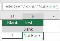
=IF(D3=»»,»Blank»,»Not Blank»)

This formula says IF(D3 is nothing, then return «Blank», otherwise «Not Blank»). Here is an example of a very common method of using «» to prevent a formula from calculating if a dependent cell is blank:

=IF(D3=»»,»»,YourFormula())

IF(D3 is nothing, then return nothing, otherwise calculate your formula).

Need more help?

Источник

Explanation

In this example, the goal is to create a formula that will return «Done» in column E when a cell in column D contains a value. In other words, if the cell in column D is «not blank», then the formula should return «Done». In the worksheet shown, column D is is used to record the date a task was completed. Therefore, if the column contains a date (i.e. is not blank), we can assume the task is complete. This problem can be solved with the IF function alone or with the IF function and the ISBLANK function. It can also be solved with the LEN function. All three approaches are explained below.

IF function

The IF function runs a logical test and returns one value for a TRUE result, and another value for a FALSE result. You can use IF to test for a blank cell like this:

=IF(A1="",TRUE) // IF A1 is blank
=IF(A1<>"",TRUE) // IF A1 is not blank

In the first example, we test if A1 is empty with =»». In the second example, the <> symbol is a logical operator that means «not equal to», so the expression A1<>»» means A1 is «not empty». In the worksheet shown, we use the second idea in cell E5 like this:

=IF(D5<>"","Done","")

If D5 is «not empty», the result is «Done». If D5 is empty, IF returns an empty string («») which displays as nothing. As the formula is copied down, it returns «Done» only when a cell in column D contains a value. To display both «Done» and «Not done», you can adjust the formula like this:

=IF(D5<>"","Done","Not done")

ISBLANK function

Another way to solve this problem is with the ISBLANK function. The ISBLANK function returns TRUE when a cell is empty and FALSE if not. To use ISBLANK directly, you can rewrite the formula like this:

=IF(ISBLANK(D5),"","Done")

Notice the TRUE and FALSE results have been swapped. The logic now is if cell D5 is blank. To maintain the original logic, you can nest ISBLANK inside the NOT function like this:

=IF(NOT(ISBLANK(D5)),"Done","")

The NOT function simply reverses the result returned by ISBLANK.

LEN function

One problem with testing for blank cells in Excel is that ISBLANK(A1) or A1=»» will both return FALSE if A1 contains a formula that returns an empty string. In other words, if a formula returns an empty string in a cell, Excel interprets the cell as «not empty». To work around this problem, you can use the LEN function to test for characters in a cell like this:

=IF(LEN(A1)>0,TRUE)

This is a much more literal formula. We are not asking Excel if A1 is blank, we are literally counting the characters in A1. The LEN function will return a positive number only when a cell contains actual characters.

Источник

EXCEL FORMULA 1. If a cell is not blank using the IF function

EXCEL

Hard coded formula

Cell reference formula

GENERIC FORMULA

=IF(cell_ref<>»», value_if_true, value_if_false)

ARGUMENTS
cell_ref: A cell that you want to check if it’s not blank.
value_if_true: Return a value if the cell that is being tested is not blank.
value_if_false: Return a value if the cell that is being tested is blank.

GENERIC FORMULA

=IF(cell_ref<>»», value_if_true, value_if_false)

EXPLANATION

This formula uses the IF function with a test criteria of two double quotation marks («»), without any value inserted between them and ‘does not equal to’ sign (<>) in front of them, to assess if a cell is not empty and return a specific value. The expression <>»» means «not empty». If a cell is not blank the formula will return a value that has been assigned as the true value, alternatively if a cell is blank the formula will return a value assigned as the false value.

With this formula you can enter the values, that will be returned if the cell is empty or not, directly into the formula or reference them to specific cells that capture these values.

Click on either the Hard Coded or Cell Reference button to view the formula that has the return values directly entered into the formula or referenced to specific cells that capture these values, respectively.

In this example the formula tests if a specific cell is not blank. If the cell is not blank the formula will return a value of «Yes» (hard coded example) or value in cell C5 (cell reference example). If the cell is empty the formula will return a value of «No» (hard coded example) or value in cell C6 (cell reference example).

If you are using the formula with values entered directly in the formula and want to return a numerical value, instead of a text value, you do not need to apply the double quotation marks around the values that are to be returned e.g. (=IF(C5<>»»,1,0)).

EXCEL FORMULA 2. If a cell is not blank using the IF, NOT and ISBLANK functions

EXCEL

Hard coded formula

Cell reference formula

GENERIC FORMULA

=IF(NOT(ISBLANK(cell_ref)), value_if_true, value_if_false)

ARGUMENTS
cell_ref: A cell that you want to check if it’s blank.
value_if_true: Value to be returned if the cell that is being tested is blank.
value_if_false: Value to be returned if the cell that is being tested is not blank.

GENERIC FORMULA

=IF(NOT(ISBLANK(cell_ref)), value_if_true, value_if_false)

EXPLANATION

This formula uses a combination of the IF, NOT and ISBLANK functions to assess if a cell is not blank and return a specific value. Unlike the first formula, which uses the double quotation marks («») to test if the selected cell is not blank, this formula uses the NOT and ISBLANK functions. If the cell is not blank the ISBLANK function will return FALSE, alternatively it will return TRUE. The NOT function will then return the opposite to what the ISBLANK function has returned. Therefore, if the cell is not blank the combination of the NOT and ISBLANK function will return a TRUE value. The formula will then return a value that has been assigned as the true value, alternatively if the cell is blank the formula will return a value assigned as the false value.

With this formula you can enter the values, that will be returned if the cell is empty or not, directly into the formula or reference them to specific cells that capture these values.

VBA CODE 1. If a cell is not blank using the If Statement

VBA

Hard coded against single cell

Sub If_a_cell_is_not_blank()

Dim ws As Worksheet

Set ws = Worksheets(«Analysis»)

If ws.Range(«C5») <> «» Then

ws.Range(«D5») = «Yes»

Else

ws.Range(«D5») = «No»

End If

End Sub

Cell reference against single cell

Sub If_a_cell_is_not_blank()

Dim ws As Worksheet

Set ws = Worksheets(«Analysis»)

If ws.Range(«C9») <> «» Then

ws.Range(«D9») = ws.Range(«C5»)

Else

ws.Range(«D9») = ws.Range(«C6»)

End If

End Sub

Hard coded against range of cells

Sub If_a_cell_is_not_blank()

Dim ws As Worksheet

Set ws = Worksheets(«Analysis»)

For x = 5 To 11

If ws.Cells(x, 3) <> «» Then

ws.Cells(x, 4) = «Yes»

Else

ws.Cells(x, 4) = «No»

End If

Next x

End Sub

Cell reference against range of cells

Sub If_a_cell_is_not_blank()

Dim ws As Worksheet

Set ws = Worksheets(«Analysis»)

For x = 9 To 15

If ws.Cells(x, 3) <> «» Then

ws.Cells(x, 4) = ws.Range(«C5»)

Else

ws.Cells(x, 4) = ws.Range(«C6»)

End If

Next x

End Sub

KEY PARAMETERS
Output Range: Select the output range by changing the cell reference («D5») in the VBA code.
Cell to Test: Select the cell that you want to check if it’s not blank by changing the cell reference («C5») in the VBA code.
Worksheet Selection: Select the worksheet which captures the cells that you want to test if they are not blank and return a specific value by changing the Analysis worksheet name in the VBA code. You can also change the name of this object variable, by changing the name ‘ws’ in the VBA code.
True and False Results: In this example if a cell is not blank the VBA code will return a value of «Yes». If a cell is blank the VBA code will return a value of «No». Both of these values can be changed to whatever value you desire by directly changing them in the VBA code.

NOTES
Note 1: If the cell that is being tested is returning a value of («») this VBA code will identify the cell as blank.
Note 2: If your True or False result is a text value it will need to be captured within quotation marks («»). However, if the result is a numeric value, you can enter it without the use of quotation marks.

KEY PARAMETERS
Output Range: Select the output range by changing the cell reference («D9») in the VBA code.
Cell to Test: Select the cell that you want to check if it’s not blank by changing the cell reference («C9») in the VBA code.
Worksheet Selection: Select the worksheet which captures the cells that you want to test if they are not blank and return a specific value by changing the Analysis worksheet name in the VBA code. You can also change the name of this object variable, by changing the name ‘ws’ in the VBA code.
True and False Results: In this example if a cell is not blank the VBA code will return a value stored in cell C5. If a cell is blank the VBA code will return a value stored in cell C6. Both of these values can be changed to whatever value you desire by either referencing to a different cell that captures the value that you want to return or change the values in those cells.

NOTES
Note 1: If the cell that is being tested is returning a value of («») this VBA code will identify the cell as blank.

KEY PARAMETERS
Output and Test Range: Select the output rows and the rows that captures the cells that are to be tested by changing the x values (5 to 11). This example assumes that both the output and the associated test cell will be in the same row.
Test Column: Select the column that captures the cells that are to be tested by changing number 3, in ws.Cells(x, 3).
Output Column: Select the output column by changing number 4, in ws.Cells(x, 4).
Worksheet Selection: Select the worksheet which captures the cells that you want to test if they are not blank and return a specific value by changing the Analysis worksheet name in the VBA code. You can also change the name of this object variable, by changing the name ‘ws’ in the VBA code.
True and False Results: In this example if a cell is not blank the VBA code will return a value of «Yes». If a cell is blank the VBA code will return a value of «No». Both of these values can be changed to whatever value you desire by directly changing them in the VBA code.

KEY PARAMETERS
Output and Test Range: Select the output rows and the rows that captures the cells that are to be tested by changing the x values (9 to 15). This example assumes that both the output and the associated test cell will be in the same row.
Test Column: Select the column that captures the cells that are to be tested by changing number 3, in ws.Cells(x, 3).
Output Column: Select the output column by changing number 4, in ws.Cells(x, 4).
Worksheet Selection: Select the worksheet which captures the cells that you want to test if they are not blank and return a specific value by changing the Analysis worksheet name in the VBA code. You can also change the name of this object variable, by changing the name ‘ws’ in the VBA code.
True and False Results: In this example if a cell is not blank the VBA code will return a value stored in cell C5. If a cell is blank the VBA code will return a value stored in cell C6. Both of these values can be changed to whatever value you desire by either referencing to a different cell that captures the value that you want to return or change the values in those cells.

NOTES
Note 1: If the cell that is being tested is returning a value of («») this VBA code will identify the cell as blank.

VBA CODE 2. If a cell is not blank using Not and IsEmpty

VBA

Hard coded against single cell

Sub If_a_cell_is_not_blank_using_Not_and_IsEmpty()

Dim ws As Worksheet

Set ws = Worksheets(«Analysis»)

If Not (IsEmpty(ws.Range(«C5»)))Then

ws.Range(«D5») = «Yes»

Else

ws.Range(«D5») = «No»

End If

End Sub

Cell reference against single cell

Sub If_a_cell_is_not_blank_using_Not_and_IsEmpty()

Dim ws As Worksheet

Set ws = Worksheets(«Analysis»)

If Not (IsEmpty(ws.Range(«C9»)))Then

ws.Range(«D9») = ws.Range(«C5»)

Else

ws.Range(«D9») = ws.Range(«C6»)

End If

End Sub

Hard coded against range of cells

Sub If_a_cell_is_not_blank_using_Not_and_IsEmpty()

Dim ws As Worksheet

Set ws = Worksheets(«Analysis»)

For x = 5 To 11

If Not (IsEmpty(ws.Cells(x, 3))) Then

ws.Cells(x, 4) = «Yes»

Else

ws.Cells(x, 4) = «No»

End If

Next x

End Sub

Cell reference against range of cells

Sub If_a_cell_is_not_blank_using_Not_and_IsEmpty()

Dim ws As Worksheet

Set ws = Worksheets(«Analysis»)

For x = 9 To 15

If Not (IsEmpty(ws.Cells(x, 3))) Then

ws.Cells(x, 4) = ws.Range(«C5»)

Else

ws.Cells(x, 4) = ws.Range(«C6»)

End If

Next x

End Sub

NOTES
Note 1: If the cell that is being tested is returning a value of («») this VBA code will identify the cell as not blank.
Note 2: If your True or False result is a text value it will need to be captured within quotation marks («»). However, if the result is a numeric value, you can enter it without the use of quotation marks.

NOTES
Note 1: If the cell that is being tested is returning a value of («») this VBA code will identify the cell as not blank.

NOTES
Note 1: If the cell that is being tested is returning a value of («») this VBA code will identify the cell as blank.

VBA CODE 3. If a cell is not blank using vbNullString

VBA

Hard coded against single cell

Sub If_a_cell_is_not_blank_using_vbNullString()

Dim ws As Worksheet

Set ws = Worksheets(«Analysis»)

If ws.Range(«C5») <> vbNullString Then

ws.Range(«D5») = «Yes»

Else

ws.Range(«D5») = «No»

End If

End Sub

Cell reference against single cell

Sub If_a_cell_is_not_blank_using_vbNullString()

Dim ws As Worksheet

Set ws = Worksheets(«Analysis»)

If ws.Range(«C9») <> vbNullString Then

ws.Range(«D9») = ws.Range(«C5»)

Else

ws.Range(«D9») = ws.Range(«C6»)

End If

End Sub

Hard coded against range of cells

Sub If_a_cell_is_not_blank_using_vbNullString()

Dim ws As Worksheet

Set ws = Worksheets(«Analysis»)

For x = 5 To 11

If ws.Cells(x, 3) <> vbNullString Then

ws.Cells(x, 4) = «Yes»

Else

ws.Cells(x, 4) = «No»

End If

Next x

End Sub

Cell reference against range of cells

Sub If_a_cell_is_not_blank_using_vbNullString()

Dim ws As Worksheet

Set ws = Worksheets(«Analysis»)

For x = 9 To 15

If ws.Cells(x, 3) <> vbNullString Then

ws.Cells(x, 4) = ws.Range(«C5»)

Else

ws.Cells(x, 4) = ws.Range(«C6»)

End If

Next x

End Sub

NOTES
Note 1: If the cell that is being tested is returning a value of («») this VBA code will identify the cell as blank.

KEY PARAMETERS
Output and Test Rows: Select the output rows and the rows that captures the cells that are to be tested by changing the x values (5 to 11). This example assumes that both the output and the associated test cell will be in the same row.
Test Column: Select the column that captures the cells that are to be tested by changing number 3, in ws.Cells(x, 3).
Output Column: Select the output column by changing number 4, in ws.Cells(x, 4).
Worksheet Selection: Select the worksheet which captures the cells that you want to test if they are not blank and return a specific value by changing the Analysis worksheet name in the VBA code. You can also change the name of this object variable, by changing the name ‘ws’ in the VBA code.
True and False Results: In this example if a cell is not blank the VBA code will return a value of «Yes». If a cell is blank the VBA code will return a value of «No». Both of these values can be changed to whatever value you desire by directly changing them in the VBA code.

KEY PARAMETERS
Output and Test Rows: Select the output rows and the rows that captures the cells that are to be tested by changing the x values (9 to 15). This example assumes that both the output and the associated test cell will be in the same row.
Test Column: Select the column that captures the cells that are to be tested by changing number 3, in ws.Cells(x, 3).
Output Column: Select the output column by changing number 4, in ws.Cells(x, 4).
Worksheet Selection: Select the worksheet which captures the cells that you want to test if they are not blank and return a specific value by changing the Analysis worksheet name in the VBA code. You can also change the name of this object variable, by changing the name ‘ws’ in the VBA code.
True and False Results: In this example if a cell is not blank the VBA code will return a value stored in cell C5. If a cell is blank the VBA code will return a value stored in cell C6. Both of these values can be changed to whatever value you desire by either referencing to a different cell that captures the value that you want to return or change the values in those cells.

NOTES
Note 1: If the cell that is being tested is returning a value of («») this VBA code will identify the cell as blank.

Источник

There are many ways to force excel for calculating a formula only if given cell/s are not blank. In this article, we will explore all the methods of calculating only «if not blank» condition.
So to demonstrate all the cases, I have prepared below data
0024
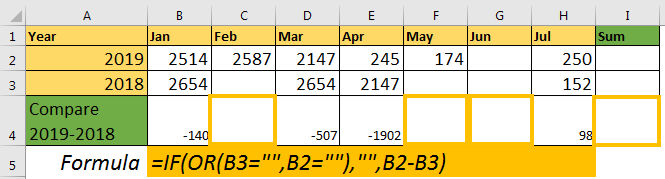
In row 4, I want the difference of months of years 2109 and 2018. For that, I will subtract 2018’s month’s data from 2019’s month’s data. The condition is, if either cell is blank, there should be no calculation. Let’s explore in how many ways you can force excel, if cell is not blank.

Calculate If Not Blank using IF function with OR Function.
The first function we think of is IF function, when it comes to conditional output. In this example, we will use IF and OR function together.
So if you want to calculate if all cells are non blank then use below formula.
Write this formula in cell B4 and fill right (CTRL+R).

=IF(OR(B3=»»,B2=»»),»»,B2-B3)

00025
How Does It work?
The OR function checks if B3 and B2 are blank or not. If either of the cell is blank, it returns TRUE. Now, for True, IF is printing “” (nothing/blank) and for False, it is printing the calculation.

The same thing can be done using IF with AND function, we just need to switch places of True Output and False Output.

=IF(AND(B3<>»»,B2<>»»),B2-B3,»»)

In this case, if any of the cells is blank, AND function returns false. And then you know how IF treats the false output.

Using the ISBLANK function
In the above formula, we are using cell=”” to check if the cell is blank or not. Well, the same thing can be done using the ISBLANK function.

=IF(OR(ISBLANK(B3),ISBLANK(B2)),””,B2-B3)

It does the same “if not blank then calculate” thing as above. It’s just uses a formula to check if cell is blank or not.

Calculate If Cell is Not Blank Using COUNTBLANK
In above example, we had only two cells to check. But what if we want a long-range to sum, and if the range has any blank cell, it should not perform calculation. In this case we can use COUNTBLANK function.

=IF(COUNTBLANK(B2:H2),»»,SUM(B2:H2))

Here, count blank returns the count blank cells in range(B2:H2). In excel, any value grater then 0 is treated as TRUE. So, if ISBLANK function finds a any blank cell, it returns a positive value. IF gets its check value as TRUE. According to the above formula, if prints nothing, if there is at least one blank cell in the range. Otherwise, the SUM function is executed.

Using the COUNTA function
If you know, how many nonblank cells there should be to perform an operation, then COUNTA function can also be used.
For example, in range B2:H2, I want to do SUM if none of the cells are blank.
So there is 7 cell in B2:H2. To do calculation only if no cells are blank, I will write below formula.

=IF(COUNTA(B3:H3)=7,SUM(B3:H3),»»)

As we know, COUNTA function returns a number of nonblank cells in the given range. Here we check the non-blank cell are 7. If they are no blank cells, the calculation takes place otherwise not.

This function works with all kinds of values. But if you want to do operation only if the cells have numeric values only, then use COUNT Function instead.

So, as you can see that there are many ways to achieve this. There’s never only one path. Choose the path that fits for you. If you have any queries regarding this article, feel free to ask in the comments section below.

Related Articles:

How to Calculate Only If Cell is Not Blank in Excel

Adjusting a Formula to Return a Blank

Checking Whether Cells in a Range are Blank, and Counting the Blank Cells

SUMIF with non-blank cells

Only Return Results from Non-Blank Cells

Popular Articles

50 Excel Shortcut to Increase Your Productivity : Get faster at your task. These 50 shortcuts will make you work even faster on Excel.

How to use the VLOOKUP Function in Excel : This is one of the most used and popular functions of excel that is used to lookup value from different ranges and sheets.

How to use the COUNTIF function in Excel : Count values with conditions using this amazing function. You don’t need to filter your data to count specific values. Countif function is essential to prepare your dashboard.

How to use the SUMIF Function in Excel : This is another dashboard essential function. This helps you sum up values on specific conditions.

Источник

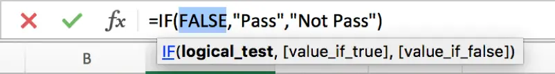
IF function is frequently used in Excel worksheet to return you expect “true value” or “false value” based on the result of created logical test. If you want to see if a cell is blank or not, and leave some comments for not blank cells, you can build a formula with IF function, IF function can return “value if not blank” or “value if blank” based on test “if cell is NOT BLANK”. See example below.

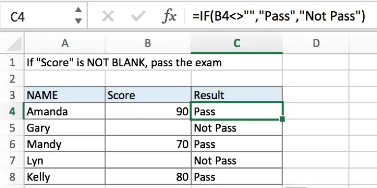
In above example, if cell is not blank in B column for a student, we think he passed the exam, formula returns result of true “Pass”, otherwise for a student, if there is no score in B column, we can assume that he didn’t pass the exam, so formula retrieves false value from the two results and returns “Not Pass” for him.

Table of Contents

FORMULA
EXPLANATION
ISBLANK Function
- Related Functions

FORMULA

To test if cell equals a certain text string, the generic formula is:

=IF(A1<>””,”if not blank value”,”blank value”)

Formula in this example:

=IF(B4<>””,”Pass”,”Not Pass”)

EXPLANATION

In this example, for a student, if cell in “Score” column is not blank, that means he passed the exam, in this case, we want to fill “Pass” in “Result” column. On the other side, if cell is blank, we want to fill “Not pass” for those students who failed the exam. So, there are two results by design, pick which one from the two result is based on the result of the logical test “if cell is blank or not”, in Excel, IF function can handle this case effectively.

IF function allows you to create a logical comparison between your value and reference value (for example “A1>0”), and set true value and false value what you expect to return as test results. IF function returns one of the two results based on logical comparison result.

Syntax: IF(logica_test,[value_if_true],[value_if_false])

To test if B4 is not blank, we can directly create a logical comparison B4<>””. The symbol <> is a logical operator that means “not equal to”. And double quotes “” represents “Empty”, there is no need to add an extra space between “”, but double quotes “” should not be ignored. If missing double quotes, Excel will prompts warning message that the formula you typed contains an error, if you ignore the error, #VALUE! is displayed in cell. Above all, B4<>”” means B4 is not equal to empty.

Besides, for the two arguments “value_if_true” and “value_if_false”, we set “Pass” and “Not Pass” separately. So the formula is:

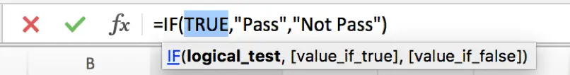
In this example, B4 is not a blank cell, logical test B4<>”” is true, so IF function evaluates True value “Pass” to C4.

For B5, B5 is a blank cell, B5<>”” is false, so IF retrieves False value “Not Pass” to C5.

In IF, true value and false value can be set as empty string “”, a text, a number or a formula, you can set what you expect to these two values.

ISBLANK Function

You can also use ISBLANK function to test if a cell is blank or not. In the formula, we can use ISBLANK(B4) to replace original logical test B4<>””. But we should be aware that ISBLANK function is to test if a cell is blank, so it returns true value if it detects that a cell is blank. So, the two results of true and false should be reversed.

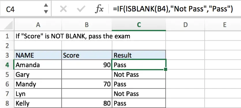
If you want to keep the sequence of your two results, you can add NOT function before ISBLANK.

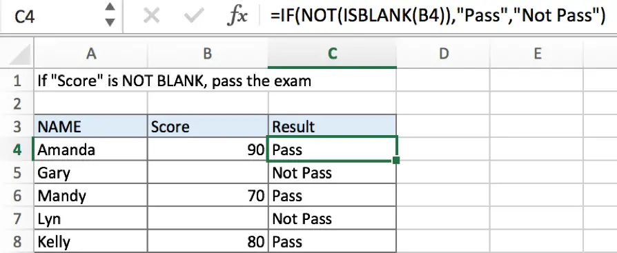
Excel ISBLANK function
The Excel ISBLANK function returns TRUE if the value is blank or null.The syntax of the ISBLANK function is as below:= ISBLANK (value)…
Excel IF function
The Excel IF function perform a logical test to return one value if the condition is TRUE and return another value if the condition is FALSE. The IF function is a build-in function in Microsoft Excel and it is categorized as a Logical Function.The syntax of the IF function is as below:= IF (condition, [true_value], [false_value])….

Источник

We can determine if a cell is not blank in Excel by either using the IF function or by using the IF and ISBLANK function combined. This tutorial will assist all levels of Excel users in both methods to identify non-blank cells

Figure 1. Final result: Determine if a cell is not blank in Excel

IF Function in Excel

IF function evaluates a given logical test and returns a TRUE or a FALSE

Syntax

=IF(logical_test, [value_if_true], [value_if_false])

The arguments “value_if_true” and “value_if_false” are optional. If left blank, the function will return TRUE if the logical test is met, and FALSE if otherwise.

ISBLANK Function in Excel

ISBLANK function is more straightforward. It tests whether a value or a cell is blank or not.

Syntax

=ISBLANK(value)

The function returns TRUE if the value is blank; FALSE if otherwise

Setting up the Data

Below is a list of Projects and a column for Date Completed. We want to know if column C for the “Date Completed” is blank or not.

Figure 2. Sample data to determine if a cell is not blank

Determine If a Cell is Not Blank

Using the IF function

In cell D3, enter the formula:

=IF(C3<>"","Not blank","Blank")

The symbol <> in Excel means “not equal to”
“” in Excel means empty string, or blank
C3<>”” means C3 is not equal to blank, or C3 is not blank

This formula returns “Not blank” because cell C3 is not blank. It has the value “July 26, 2018”.

Figure 3. Entering the IF formula to determine if a cell is not blank

In cell D4, enter the formula:

=IF(C4<>"","Not blank","Blank")

The result is “Blank” because cell D4 is empty.

Figure 4. Output: Using IF to determine if a cell is not blank

Using the IF and ISBLANK function

In cell D5, enter the formula:

=IF(ISBLANK(C5),"Blank","Not Blank")

ISBLANK evaluates whether cell C5 is blank or not
If the ISBLANK function returns TRUE, the formula will return “Blank”; otherwise, it returns “Not Blank”
The result is “Blank” because C5 is empty

Figure 5. Final result: Using IF and ISBLANK to determine if a cell is not blank

Note

We can customize the action that the IF function will return depending on the logical test results.

Example

We want to return the status “Completed” if the cell in column C is not blank, and “In Progress” if otherwise.

Enter the following formula:

In cell D3: =IF(C3<>"","Completed","In Progress")

In cell D4: =IF(C4<>"","Completed","In Progress")

In cell D5: =IF(ISBLANK(C5),"In Progress","Completed")

In cell D6: =IF(ISBLANK(C6),"In Progress","Completed")

Figure 6. Final result: Using IF and ISBLANK to determine the status of a project

Most of the time, the problem you will need to solve will be more complex than a simple application of a formula or function. If you want to save hours of research and frustration, try our live Excelchat service! Our Excel Experts are available 24/7 to answer any Excel question you may have. We guarantee a connection within 30 seconds and a customized solution within 20 minutes.

Are you still looking for help with the IF function? View our comprehensive round-up of IF function tutorials here.

Источник

Home / Excel Formulas / IF Cell is Blank (Empty) using IF + ISBLANK

In Excel, if you want to check if a cell is blank or not, you can use a combination formula of IF and ISBLANK. These two formulas work in a way where ISBLANK checks for the cell value and then IF returns a meaningful full message (specified by you) in return.

In the following example, you have a list of numbers where you have a few cells blank.

Formula to Check IF a Cell is Blank or Not (Empty)

First, in cell B1, enter IF in the cell.
Now, in the first argument, enter the ISBLANK and refer to cell A1 and enter the closing parentheses.
Next, in the second argument, use the “Blank” value.
After that, in the third argument, use “Non-Blank”.
In the end, close the function, hit enter, and drag the formula up to the last value that you have in the list.

As you can see, we have the value “Blank” for the cell where the cell is empty in column A.

=IF(ISBLANK(A1),"Blank","Non-Blank")

Now let’s understand this formula. In the first part where we have the ISBLANK which checks if the cells are blank or not.

And, after that, if the value returned by the ISBLANK is TRUE, IF will return “Blank”, and if the value returned by the ISBLANK is FALSE IF will return “Non_Blank”.

Alternate Formula

You can also use an alternate formula where you just need to use the IF function. Now in the function, you just need to specify the cell where you want to test the condition and then use an equal operator with the blank value to create a condition to test.

And you just need to specify two values that you want to get the condition TRUE or FALSE.

Download Sample File

Ready

And, if you want to Get Smarter than Your Colleagues check out these FREE COURSES to Learn Excel, Excel Skills, and Excel Tips and Tricks.

Источник

I would like to write an IF statement, where the cell is left blank if the condition is FALSE.
Note that, if the following formula is entered in C1 (for which the condition is false) for example:

 =IF(A1=1,B1,"")

and if C1 is tested for being blank or not using =ISBLANK(C1), this would return FALSE, even if C1 seems to be blank. This means that the =IF(A1=1,B1,"") formula does not technically leave the cells blank if the condition is not met.

Any thoughts as to a way of achieving that? Thanks,

Vegard

3,5572 gold badges22 silver badges40 bronze badges

asked Sep 12, 2013 at 15:09

Unfortunately, there is no formula way to result in a truly blank cell, "" is the best formulas can offer.

I dislike ISBLANK because it will not see cells that only have "" as blanks. Instead I prefer COUNTBLANK, which will count "" as blank, so basically =COUNTBLANK(C1)>0 means that C1 is blank or has "".

If you need to remove blank cells in a column, I would recommend filtering on the column for blanks, then selecting the resulting cells and pressing Del. After which you can remove the filter.

answered Sep 12, 2013 at 15:31

tigeravatartigeravatar

26.1k5 gold badges28 silver badges38 bronze badges

Try this instead

=IF(ISBLANK(C1),TRUE,(TRIM(C1)=""))

This will return true for cells that are either truly blank, or contain nothing but white space.

See this post for a few other options.

edit

To reflect the comments and what you ended up doing: Instead of evaluating to «» enter another value such as ‘deleteme’ and then search for ‘deleteme’ instead of blanks.

=IF(ISBLANK(C1),TRUE,(TRIM(C1)="deleteme"))

answered Sep 12, 2013 at 15:12

Automate ThisAutomate This

30.5k11 gold badges62 silver badges82 bronze badges

I wanted to add that there is another possibility — to use the function na().

e.g. =if(a2 = 5,"good",na());

This will fill the cell with #N/A and if you chart the column, the data won’t be graphed. I know it isn’t «blank» as such, but it’s another possibility if you have blank strings in your data and "" is a valid option.

Also, count(a:a) will not count cells which have been set to n/a by doing this.

answered Apr 2, 2016 at 0:03

user3791372user3791372

4,3455 gold badges43 silver badges77 bronze badges

If you want to use a phenomenical (with a formula in it) blank cell to make an arithmetic/mathematical operation, all you have to do is use this formula:

=N(C1)

assuming C1 is a «blank» cell

answered Mar 11, 2017 at 15:07

NickNick

9561 gold badge10 silver badges20 bronze badges

You could try this.

=IF(A1=1,B1,TRIM(" "))

If you put this formula in cell C1, then you could test if this cell is blank in another cells

=ISBLANK(C1)

You should see TRUE. I’ve tried on Microsoft Excel 2013.
Hope this helps.

answered Mar 19, 2020 at 2:48

I’ve found this workaround seems to do the trick:

Modify your original formula:

=IF(A1=1,B1,"filler")

Then select the column, search and replace «filler» with nothing. The cells you want to be blank/empty are actually empty and if you test with «ISBLANK» it will return TRUE. Not the most elegant, but it’s quick and it works.

mdml

22.2k8 gold badges58 silver badges65 bronze badges

answered Feb 7, 2014 at 19:20

The easiest solution is to use conditional formatting if the IF Statement comes back false to change the font of the results cell to whatever color background is. Yes, technically the cell isn’t blank, but you won’t be able to see it’s contents.

answered Sep 27, 2014 at 0:13

This shall work (modification on above, workaround, not formula)

Modify your original formula:
=IF(A1=1,B1,»filler»)

Put filter on spreadsheet, choose only «filler» in column B, highlight all the cells with «filler» in them, hit delete, remove filter

answered Apr 28, 2015 at 19:55

You can do something like this to show blank space:

=IF(AND((E2-D2)>0)=TRUE,E2-D2," ")

Inside if before first comma is condition then result and return value if true and last in value as blank if condition is false

J-Alex

6,72510 gold badges45 silver badges61 bronze badges

answered Jun 21, 2017 at 7:57

The formula in C1

=IF(A1=1,B1,"")

is either giving an answer of «» (which isn’t treated as blank) or the contents of B1.

If you want the formula in D1 to show TRUE if C1 is «» and FALSE if C1 has something else in then use the formula

=IF(C2="",TRUE,FALSE)

instead of ISBLANK

answered Sep 15, 2017 at 13:42

ChrisMChrisM

1,5766 gold badges17 silver badges28 bronze badges

Here is what I do

=IF(OR(ISBLANK(AH38),AH38=""),"",IF(AI38=0,0,AH38/AI38))

Use the OR condition OR(ISBLANK(cell), cell=»»)

answered Dec 24, 2018 at 2:04

TalhaTalha

1,51617 silver badges15 bronze badges

To Validate data in column A for Blanks

Step 1: Step 1: B1=isblank(A1)

Step 2: Drag the formula for the entire column say B1:B100; This returns Ture or False from B1 to B100 depending on the data in column A

Step 3: CTRL+A (Selct all), CTRL+C (Copy All) , CRTL+V (Paste all as values)

Step4: Ctrl+F ; Find and replace function Find «False», Replace «leave this blank field» ; Find and Replace ALL

There you go Dude!

answered Dec 6, 2014 at 23:59

Instead of using «», use 0. Then use conditional formating to color 0 to the backgrounds color, so that it appears blank.

Since blank cells and 0 will have the same behavior in most situations, this may solve the issue.

answered Jun 24, 2014 at 14:13

This should should work: =IF(A1=1, B1)

The 3rd argument stating the value of the cell if the condition is not met is optional.

answered Nov 18, 2014 at 10:04

Источник

Чтобы выполнить действие только тогда, когда ячейка не пуста (содержит какие-то значения), вы можете использовать формулу, основанную на функции ЕСЛИ.
В примере ниже столбец F содержит даты завершения закупок шоколада.
Поскольку даты для Excel — это числа, то наша задача состоит в том, чтобы проверить в ячейке наличие числа.
Формула в ячейке F3:
=ЕСЛИ(СЧЁТЗ(D3:D9)=7,СУММ(C3:C9),»»)

Как работает эта формула?

Функция СЧЕТЗ (английский вариант — COUNTA) подсчитывает количество значений (текстовых, числовых и логических) в диапазоне ячеек Excel.

Если мы знаем количество значений в диапазоне, то легко можно составить условие. Если число значений равно числу ячеек, значит, пустых ячеек нет и можно производить вычисление.

Если равенства нет, значит есть хотя бы одна пустая ячейка, и вычислять нельзя.

Согласитесь, что нельзя назвать этот способ определения наличия пустых ячеек удобным. Ведь число строк в таблице может измениться, и нужно будет менять формулу: вместо цифры 7 ставить другое число.

Давайте рассмотрим и другие варианты. В ячейке F6 записана большая формула —

=ЕСЛИ(ИЛИ(ЕПУСТО(D3),ЕПУСТО(D4),ЕПУСТО(D5),ЕПУСТО(D6),ЕПУСТО(D7),ЕПУСТО(D8),ЕПУСТО(D9)),»»,СУММ(C3:C9))

Функция ЕПУСТО (английский вариант — ISBLANK) проверяет, не ссылается ли она на пустую ячейку. Если это так, то возвращает ИСТИНА.

Функция ИЛИ (английский вариант — OR) позволяет объединить условия и указать, что нам достаточно того, чтобы хотя бы одна функция ЕПУСТО обнаружила пустую ячейку. В этом случае никаких вычислений не производим и функция ЕСЛИ возвращает пустую строку. В противном случае — производим вычисления.

Все достаточно просто, но перечислять кучу ссылок на ячейки не слишком удобно. К тому же, здесь, как и в предыдущем случае, формула не масштабируема: при изменении таблицы она нуждается в корректировке. Это не слишком удобно, да и забыть можно сделать это.

Рассмотрим теперь более универсальные решения.

=ЕСЛИ(СЧИТАТЬПУСТОТЫ(D3:D9),»»,СУММ(C3:C9))

В качестве условия в функции ЕСЛИ мы используем СЧИТАТЬПУСТОТЫ (английский вариант — COUNTBLANK). Она возвращает количество пустых ячеек, но любое число больше 0 Excel интерпретирует как ИСТИНА.

И, наконец, еще одна формула Excel, которая позволит производить расчет только при наличии непустых ячеек.

=ЕСЛИ(ЕЧИСЛО(D3:D9),СУММ(C3:C9),»»)

Функция ЕЧИСЛО ( или ISNUMBER) возвращает ИСТИНА, если ссылается на число. Естественно, при ссылке на пустую ячейку возвратит ЛОЖЬ.

А теперь посмотрим, как это работает. Заполним таблицу недостающим значением.

Как видите, все наши формулы рассчитаны и возвратили одинаковые значения.

А теперь рассмотрим как проверить, что ячейки не пустые, если в них могут быть записаны не только числа, но и текст.

Итак, перед нами уже знакомая формула
=ЕСЛИ(СЧЁТЗ(D3:D9)=7,СУММ(C3:C9),»»)
Для функции СЧЕТЗ не имеет значения, число или текст используются в ячейке Excel.
=ЕСЛИ(СЧИТАТЬПУСТОТЫ(D3:D9),»»,СУММ(C3:C9))
То же можно сказать и о функции СЧИТАТЬПУСТОТЫ.

А вот третий вариант — к проверке условия при помощи функции ЕЧИСЛО добавляем проверку ЕТЕКСТ (ISTEXT в английском варианте). Объединяем их функцией ИЛИ.

=ЕСЛИ(ИЛИ(ЕТЕКСТ(D3:D9),ЕЧИСЛО(D3:D9)),СУММ(C3:C9),»»)

А теперь вставляем в ячейку D5 недостающее значение и проверяем, все ли работает.

Надеемся, этот материал был полезен. А вот еще несколько примеров работы с условиями и функцией ЕСЛИ в Excel.

Функция ЕСЛИ: примеры с несколькими условиями — Для того, чтобы описать условие в функции ЕСЛИ, Excel позволяет использовать более сложные конструкции. В том числе можно использовать и несколько условий. Рассмотрим на примере. Для объединения нескольких условий в… Проверка ввода данных в Excel — Подтверждаем правильность ввода галочкой. Задача: При ручном вводе данных в ячейки таблицы проверять правильность ввода в соответствии с имеющимся списком допустимых значений. В случае правильного ввода в отдельном столбце ставить… Функция ЕСЛИ: проверяем условия с текстом — Рассмотрим использование функции ЕСЛИ в Excel в том случае, если в ячейке находится текст. СодержаниеПроверяем условие для полного совпадения текста.ЕСЛИ + СОВПАДИспользование функции ЕСЛИ с частичным совпадением текста.ЕСЛИ + ПОИСКЕСЛИ… Визуализация данных при помощи функции ЕСЛИ — Функцию ЕСЛИ можно использовать для вставки в таблицу символов, которые наглядно показывают происходящие с данными изменения. К примеру, мы хотим показать, происходит рост или снижение продаж. В столбце N поставим… Как функция ЕСЛИ работает с датами? — На первый взгляд может показаться, что функцию ЕСЛИ для работы с датами можно использовать так же, как для числовых и текстовых значений, которые мы только что обсудили. К сожалению, это…

Источник: https://mister-office.ru/formuly-excel/calculate-if-not-blank.html

Как заполнить пустые ячейки в Excel?

Зачастую мы имеем таблицу в Excel, в которой присутствуют пустые ячейки. Заполнение таких ячеек вручную займет огромное количество времени.

Для заполнения пустых ячеек в таких случаях можно использовать способы, перечисленные ниже.

Способ 1: Заполнение пустых ячеек в Excel с помощью заданного значения

Вы можете заполнить пустые ячейки столбца на листе Excel с помощью указанного значения. Для это можно воспользоваться встроенными возможностями Excel, которые очень легко выполнить.

Первая функция Go To специальной особенностью Excel, а затем заполнить все пустые ячейки с заданным значением.

И этот метод настолько прост , что вы можете использовать без каких — либо специальных знаний.

Следующие шаги иллюстрируют, как заполнить пустые ячейки в Excel с помощью указанного значения.
Шаг 1: Откройте нужный лист Excel, на котором необходимо заполнить пустые ячейки.
Шаг 2: Выберите конкретный столбец, содержащий пустые ячейки.

Шаг 3: Теперь найдите кнопку Найти и выделить в меню Главная и выберите Выделить группу ячеек. Появится окно с различными вариантами. Выберите Пустые ячейки.

Шаг 4: После данного выбора все пустые ячейки в указанном диапазоне будут выделены. Теперь, не нажимая ничего, введите необходимо значение, которое нужно поместить во все пустые ячейки и нажмите Ctrl + Enter. Пустые ячейки заполнятся нужным содержимым.

Таким образом вы можете легко заполнить пустые клетки определенного столбца заданным значением. Это довольно легко сделать, поскольку не требуется какого-либо приложения или программного обеспечения.

Способ 2: Заполнение пустых ячеек в Excel значением, расположенным в ячейке выше

Этот способ пригодится в том случае, если необходимо заполнить пустые ячейки значением, находящимся в ячейке выше пустых. Для того, чтобы заполнить пустые ячейки значением предыдущей ячейки, также можно использовать возможности Excel.

Шаг 1: Откройте нужный лист Excel, который содержит пустые ячейки.

Шаг 2: Выберите диапазон ячеек, в котором нужно заполнить пустые ячейки.

Шаг 4: В строке формул наберите знак «=» и укажите ячейку, содержимым которой необходимо заполнить пустые ячейки. Далее нажмите Ctrl + Enter. Вы увидите, что все пустые ячейки заполнились значением ячейки выше. Смотрите скриншоты ниже.

Таким образом вы можете легко заполнить все пустые ячейки в листе Excel со значением над ними.

Способ 3: Заполнение пустых ячеек Excel со значением выше с помощью макроса VBA

Использование макросов сводит выполнение какой-либо команды до одного нажатия клавиши. Для заполнения пустых ячеек значением предыдущей ячейки также можно задать через макрос. Кроме того, этот макрос автоматически определяет используемый диапазон на листе, а затем он заполняет все пустые ячейки со значением над ними.

Шаг 1: Откройте рабочий лист , в котором вы хотите , чтобы заполнить все пустые ячейки со значением над ними.

Шаг 2: Теперь откройте редактор VBA, нажав Alt + F11.

Шаг 3: Щелкните правой кнопкой мыши на любом проекте и перейдите к Insert > Module. После этого вставьте следующий код VBA.

Sub FillBlankCells()

Static rngUR As Range: Set rngUR = ActiveWorkbook.ActiveSheet.UsedRange

Dim rngBlank As Range: Set rngBlank = rngUR.Find(«»)

While Not rngBlank Is Nothing

rngBlank.Value = rngBlank.Offset(-1, 0).Value

Set rngBlank = rngUR.Find(«», rngBlank)
Wend
End Sub

Шаг 4: Теперь сохраните модуль с помощью клавиши Ctrl + S, появившееся диалоговое окно с предупреждением просто проигнорируйте, нажав на кнопку Нет. Теперь вы можете задать сочетание клавиш для выполнения макроса. (меню Разработчик Макросы выберите нужный макрос Параметры Сочетание клавиш (укажите букву).

Шаг 5: На этом этапе макрокоманда готова к использованию. Чтобы использовать ее, нажмите клавишу быстрого доступа, назначенную для нее, и вы увидите результат в мгновение ока.

Таким образом вы можете легко заполнить пустые ячейки в Excel с помощью этого макроса. Тем не менее, существует недостаток использования макросов: невозможно отменить внесенные с помощью макроса изменения кнопкой Отменить ввод.

Источник: http://pro-spo.ru/internet/5196-kak-zapolnit-pustye-yachejki-v-excel

Excel говорит мне, что мои пустые ячейки не пустые

поэтому в excel я пытаюсь избавиться от пустых ячеек между моими ячейками, в которых есть информация, используя F5 для поиска пустых ячеек, затем Ctrl + — для их удаления и сдвига ячеек вверх. Но когда я пытаюсь это сделать, он говорит мне, что «клеток не найдено».

Итак, мой вопрос в том, как я могу это сделать, но с этими пустыми ячейками, которые Excel считает не пустыми? Я попытался пройти и просто нажать delete над пустыми ячейками, но у меня много данных и понял, что это займет слишком много времени. мне нужно найти способ выбрать эти «пустые» ячейки в пределах выбора данных.

заранее спасибо за вашу помощь! 🙂

откровение: некоторые пустые ячейки на самом деле не пустой! Как я покажу, ячейки могут иметь пробелы, новые строки и true empty:

чтобы найти эти ячейки быстро вы можете сделать несколько вещей.

на =CODE(A1) формула вернет значение#! если клетка действительно пуста, в противном случае вернется. Это число -номер ASCII в =CHAR(32).
если вы выделите ячейку и щелкните в строке формул и используйте курсор, чтобы выбрать все.

удаление этих:

если у вас есть только пробел в клетках они могут быть легко удалены с помощью:

пресс ctrl + h чтобы открыть find и replace.
введите одно место в найти, оставить заменить на пустой и убедитесь, что у вас есть матч всей ячейки содержание галочкой в опциях.
пресс заменить все.

если у вас newlines это сложнее и требует VBA:

щелкните правой кнопкой мыши на вкладке листа > Просмотр кода.
затем введите следующий код. Помните Chr(10) новая строка заменяет это только по мере необходимости, например » » & Char(10) это пробел и новая строка:

Sub find_newlines()
With Me.Cells
Set c = .Find(Chr(10), LookIn:=xlValues, LookAt:=xlWhole)
If Not c Is Nothing Then
firstAddress = c.Address
Do
c.Value = «»
Set c = .FindNext(c)
If c Is Nothing Then Exit Do
Loop While c.Address firstAddress
End If
End With
End Sub
Теперь запустите ваш код нажатие Ф5.

после файл поставляется: выберите диапазон интересов для повышения производительности, затем выполните следующие действия:

Sub find_newlines()
With Selection
Set c = .Find(«», LookIn:=xlValues, LookAt:=xlWhole)
If Not c Is Nothing Then
firstAddress = c.Address
Do
c.Value = «»
Set c = .FindNext(c)
If c Is Nothing Then Exit Do
Loop While c.Address firstAddress
End If
End With
End Sub

простой способ выбрать и очистить эти пустые ячейки, чтобы сделать их пустыми:

пресс ctrl + a или предварительно выберите свой диапазон
пресс ctrl + f
оставить найти пустой и выберите матч всего содержимого ячейки.
нажмите найти все
пресс ctrl + a выбрать все пустые ячейки нашли
закрыть поиск диалоговое окно
пресс backspace или удалить

Это сработало для меня:

CTR-H для поиска и замены
оставьте «найти что» пустой
изменить «заменить на» на уникальный текст, то, что вы
положительный не будет найден в другой ячейке (я использовал ‘xx’)
клик
«Заменить Все»
скопируйте уникальный текст на Шаге 3, чтобы найти то, что’
удалить уникальный текст в «заменить на»
нажмите «заменить все»

У меня была аналогичная проблема, когда разбросанные пустые ячейки из экспорта из другого приложения все еще отображались в подсчетах ячеек.

мне удалось очистить их

выбор столбцов / строк, которые я хотел очистить, а затем делать
«найти» [без текста] и» заменить » [слово выбора].
затем я сделал «найти» [слово выбора] и» заменить » на [нет текста].

он избавился от всех скрытых / фантомных персонажей в тех ячейки. Может, это сработает?

все, это довольно просто. Я пытался сделать то же самое, и это то, что сработало для меня в VBA

Range(«A1:R50»).Select ‘The range you want to remove blanks
With Selection
Selection.NumberFormat = «General»
.Value = .Value
End With

С уважением,
Ананд Ланка

Если у вас нет форматирования или формул, которые вы хотите сохранить, вы можете попробовать сохранить файл в виде текстового файла с разделителями табуляции, закрыть его и снова открыть с помощью excel. Это сработало для меня.

‘Select non blank cells
Selection.SpecialCells(xlCellTypeConstants, 23).Select
‘ REplace tehse blank look like cells to something uniqu
Selection.Replace What:=»», Replacement:=»TOBEDELETED», LookAt:=xlWhole, _
SearchOrder:=xlByRows, MatchCase:=False, SearchFormat:=False, _
ReplaceFormat:=False
‘now replace this uique text to nothing and voila all will disappear
Selection.Replace What:=»TOBEDELETED», Replacement:=»», LookAt:=xlWhole, _
SearchOrder:=xlByRows, MatchCase:=False, SearchFormat:=False, _
ReplaceFormat:=False

нашел другой способ. Установите автофильтр для все столбцы (важно или вы будете смещать данные), выбрав строку заголовка > вкладка «данные» > сортировка и фильтр — «фильтр».

Используйте раскрывающийся список в первом столбце данных, снимите флажок «выбрать все» и выберите только «(пробелы) » > [OK]. Выделите строки (Теперь все вместе) > щелкните правой кнопкой мыши > «удалить строку».

Вернитесь к раскрывающемуся меню > ‘Select all’. Престо:)

Не уверен, что это уже было сказано, но у меня была аналогичная проблема с ячейками, ничего не показывающими в них, но не пустыми при запуске формулы IsBlank ().

Я выбрал весь столбец, выбрал Find & Replace, нашел ячейки ни с чем и заменил на 0, затем снова запустил find и replace, найдя ячейки с 0 и заменив их на «».

Это решило мою проблему и позволило мне искать пустые ячейки (F5, специальные, пробелы) и удалять строки, которые были пусты….БУМ.

может не работать для каждого приложения, но это решило мою проблему.

иногда в ячейках есть пробелы, которые кажутся пустыми, но если вы нажмете F2 на ячейке, вы увидите пробелы. Вы также можете выполнить поиск таким образом, если знаете точное количество пробелов в ячейке

Это работает с цифрами.

Если ваш диапазон O8:O20, то в соседнем пустом диапазоне (например, T8: T20) введите =O8/1 и заполните. Это даст вам результат #VALUE для «пустых» ячеек, и ваш исходный номер останется прежним.

затем с выбранным диапазоном T8: 20 (CTL -*, если это еще не так) нажмите F5 и выберите специальный. В специальном диалоге выберите ошибки и нажмите кнопку ОК. Это отменит выбор фактических номеров, оставив только выбранные ячейки #VALUE. Удалите их, и у вас будут фактические пустые ячейки. Скопируйте T8:T20 и вставьте обратно через O8: O20.

по существу, поскольку пустые ячейки не работают, вам нужно преобразовать «пустые» ячейки во что-то, что может зацепиться за специальное. Любое действие, которое будет преобразовано в #VALUE, будет работать, и другие типы «ошибок» также должны поддерживаться.

мой метод похож на предложение Курта выше о сохранении его как файла с разделителями табуляции и повторном импорте.
Предполагается, что данные имеют только значения без формул.

Это, вероятно, хорошее предположение, потому что проблема «плохих» пробелов вызвана путаницей между пробелами и нулями-обычно в данных, импортированных из какого-то другого места, — поэтому не должно быть никаких формул.

Мой метод —разобрать на месте — очень похоже на сохранение в виде текстового файла и повторный импорт, но вы можете сделать это без закрытия и повторного открытия файла.

Он находится в разделе Данные > текст в Столбцы > разделители > удалить все символы синтаксического анализа (также можно выбрать текст, если хотите) > готово. Это должно заставить Excel повторно распознавать ваши данные с нуля или из текста и распознавать пробелы как действительно пустые.
Вы можете автоматизировать это в подпрограмме:

Sub F2Enter_new()
Dim rInput As Range
If Selection.Cells.Count > 1 Then Set rInput = Selection
Set rInput = Application.InputBox(Title:=»Select», prompt:=»input range», _
Default:=rInput.Address, Type:=8)
‘ Application.EnableEvents = False: Application.ScreenUpdating = False
For Each c In rInput.Columns
c.TextToColumns Destination:=Range(c.Cells(1).Address), DataType:=xlDelimited, _
TextQualifier:=xlDoubleQuote, ConsecutiveDelimiter:=False, Tab:=False, _
Semicolon:=False, Comma:=False, Space:=False, Other:=False, _
FieldInfo:=Array(1, 1), TrailingMinusNumbers:=True
Next c
Application.EnableEvents = True: Application.ScreenUpdating = True
End Sub

вы также можете включить эту прокомментированную строку, чтобы эта подпрограмма выполнялась «в фоновом режиме». Для этой подпрограммы улучшается производительность только немного (для других это действительно может помочь).
Имя-F2Enter, потому что исходный ручной метод для исправления этой проблемы «пробелов» — заставить Excel распознать формулу, нажав F2 и Enter.

вот как я исправил эту проблему без какого-либо кодирования.

выберите весь столбец, из которого я хотел удалить «пустые» ячейки.
щелкните вкладку Условное форматирование вверху.
Выберите «Новое Правило».
нажать «форматировать только ячейки, которые содержат».
изменить «между» На «равно».
нажмите на поле рядом с полем» равно».
нажмите одну из проблемных» пустых » ячеек.
клик кнопка формат.
выберите случайный цвет для заполнения коробки.
нажмите «OK».
Это должно изменить все проблемные» пустые » ячейки на цвет, который вы выбрали. Теперь щелкните правой кнопкой мыши одну из цветных ячеек и перейдите в раздел «сортировать» и «поместить выбранный цвет ячейки сверху».
это поставит все проблемные ячейки в верхней части столбца, и теперь все ваши другие ячейки останутся в исходном порядке, в котором вы их поместите. Теперь вы можете выбрать все проблемные ячейки в одной группе и нажмите кнопку Удалить ячейку сверху, чтобы избавиться от них.

самым простым решением для меня было:
1) Выберите диапазон и скопируйте его (ctrl+c)
2)Создайте новый текстовый файл (в любом месте, он будет удален в ближайшее время), откройте текстовый файл, а затем вставьте в excel информацию (ctrl+v)
3) Теперь, когда информация в Excel находится в текстовом файле, выполните select all в текстовом файле (ctrl+a), а затем скопируйте (ctrl+c)
4) перейдите к началу исходного диапазона на шаге 1 и вставьте его старая информация из копии на Шаге 3.

готово! Больше никаких фальшивых заготовок! (теперь вы можете удалить временный текстовый файл)

Goto — > Special — >blanks не любит объединенные ячейки. Попробовать unmerging клеток выше диапазона, в котором вы хотите выбрать то, болванками попробовать снова.

У меня была аналогичная проблема с получением формулы COUNTA для подсчета непустых ячеек, она считала все из них (даже пустые как непустые), я попытался =CODE (), но у них не было пробелов или новых строк.

Я обнаружил, что когда я щелкнул в ячейке, а затем щелкнул из нее, формула будет считать ячейку. У меня были тысячи ячеек, поэтому я не мог сделать это вручную.

Я написал этот оператор VBA, чтобы буквально проверить все ячейки, и если они были пустыми, то сделать их пустыми.

Игнорируйте бессмысленность этого макроса и поверьте мне, что он действительно работал, заставляя Excel распознавать пустые ячейки как пустые.

‘This checks all the cells in a table so will need to be changed if you’re using a range
Sub CreateBlanks()

Dim clientTable As ListObject
Dim selectedCell As Range

Set clientTable = Worksheets(«Client Table»).ListObjects(«ClientTable»)

For Each selectedCell In clientTable.DataBodyRange.Cells
If selectedCell = «» Then
selectedCell = «»
End If
Next selectedCell
End Sub

Источник: https://askdev.ru/q/excel-govorit-mne-chto-moi-pustye-yacheyki-ne-pustye-186301/

За 60 секунд: Как в Excel показывать нули как пустые ячейки

Когда вы работаете в Excel с большими таблицами данных, вполне вероятно, что многие из ваших данных, могут оказаться нулями.

Это обычное явление, но это может сделать вашу таблицу трудной для чтения и навигации. Нам не нужно менять все эти нули и удалять их из данных, чтобы очистить нашу таблицу.

Вместо этого мы можем просто изменить то, как они отображаются. Вместо того, чтобы показывать все эти нули, мы могли бы удалить их одним простым способом в Excel. Давайте научимся.

Как быстро отобразить ячейки Excel пустыми, если в них нуль

Примечание: просмотрите этот короткий видеоурок или следуйте шагам ниже, которые дополняют это видео.

1. Откройте файл Excel с нулевыми ячейками

Мы начинаем с файла Excel с многочисленными ячейками 0, которые мы хотим превратить в пустые.

Файл Excel с нулевыми (0) ячейками.

2. Как отключить отображение нулей в Excel

Теперь перейдите на вкладку Файл в Excel. Найдите кнопку Параметры с левой стороны и, давайте, нажмите на неё.

Теперь измените параметр Дополнительно с левой стороны. Прокрутим вниз. И посреди этих параметров, идём в поле, которое говорит: Показывать нули в ячейках, которые содержат нулевые значения. Этот параметр управляет настройками для всей книги. Нам нужно снять этот флажок и, теперь, давайте нажмем OK.

Показывать нули в ячейках, которые содержат нулевые значения.

3. Теперь Excel показывает нулевые ячейки как пустые

Когда мы вернемся к книге, вы увидите, что все нули теперь скрыты. Нулевое значение всё ещё находится внутри ячейки, но Excel меняет способ его отображения, и ячейки выглядят пустыми. Это также может быть полезно, например, для сводной таблицы.

Ячейки Excel теперь пусты, если в них ноль.

Закругляемся!

Теперь вы знаете, как изменить Excel так, что если ячейка равна 0, её можно сделать пустой при необходимости. Этот вариант полезен для того, чтобы электронные таблицы были более читабельными и сосредоточенными на значимых данных.

Более полезные учебники по Excel на Envato Tuts+

Найдите исчерпывающие уроки по Excel на Envato Tuts+, которые помогут вам лучше научиться работать с данными в электронных таблицах. У нас также есть быстрые серии по Excel в 60-секундной, чтобы быстрее изучить больше инструментов Excel.

Вот несколько уроков по Excel, на которые можно перейти в настоящее время:

- Microsoft Excel
- За 60 секунд: Как защищать ячейки, листы и книги в Excel
- Эндрю Чилдресс
1. Microsoft Excel
2. За 60 секунд: Как вставлять, удалять и прятать новые листы в Excel
3. Эндрю Чилдресс
- Microsoft Excel
- За 60 секунд: Как закреплять области и строки в Excel
- Эндрю Чилдресс

Помните: каждый инструмент Microsoft Excel, который вы изучаете, позволяют вам создавать более мощные электронные таблицы.

Источник: https://business.tutsplus.com/ru/tutorials/excel-zeros-as-blank-cells—cms-29487

microsoft-excel — Отображать пустое значение при ссылке на пустую ячейку в Excel 2010

У меня есть книга Excel 2010, в которой содержится несколько отдельных рабочих листов. Ячейки на одном из листов связаны с отдельными ячейками на двух других листах в одной книге.

Я использую ссылку на прямую ячейку, которая по существу говорит, что любое значение, введенное в конкретную ячейку на одном листе, также заполняет ячейки на двух других листах.

Я использовал функцию (=) со ссылкой на ячейку, чтобы выполнить это.

Проблема, с которой я сталкиваюсь, заключается в том, что даже если основная ячейка оставлена пустой, ячейки, которые заполняются из этой первичной ячейки, будут отображать 0, а не оставаться пустыми.

Я хочу, чтобы подчиненные ячейки оставались пустыми, если основная ячейка, с которой они связаны, пуста.

Вам нужно заставить Excel обрабатывать содержимое ячейки как текстовое значение вместо числа, которое оно делает автоматически с пустыми значениями.

=A2 & «»

Это заставит Excel сделать ссылку на ячейку текстовым значением,
тем самым предотвращая превращение заготовок в нули.

ответил wbeard52 28 апреля 2015, 07:56:10

Вот три ответа:

1) Предоставление other.cell.reference представляет собой ссылочную формулу, которую вы в настоящее время используете после = (например, Sheet17!$H$42), замените ссылку на ссылку с помощью

=IF( other.cell.reference «», other.cell.reference , «»)

2) Установите формат «Число» ваших связанных ячеек в «Пользовательский»: General;–General;.

3) В разделе «Параметры Excel», «Дополнительно» на странице «Параметры отображения для этой рабочей таблицы» снимите флажок «Показывать нуль в ячейках с нулевым значением». Предупреждение: это приведет к исчезновению всех нулей на листе.

ответил Scott 7 декабря 2012, 01:30:16

Если ваши ссылочные данные являются либо числовыми (нетекстовыми), либо пустыми, и у вас может быть 0, то это мой предпочтительный подход, только один раз вводя формулу. По общему признанию, слегка косвенный путь, но лучше всего я думаю, потому что:

вам не нужны лишние ячейки для ввода формулы, а затем ссылки на вторую ячейку
Вам не нужно вводить формулу дважды
этот метод различает нулевое значение и пустую ячейку
не требуется VBA
не требует именных диапазонов

Downfall . Если вам нужны текстовые данные, это не сработает. Для текстовых данных мой предпочтительный метод использует формат чисел, как указано в других ответах выше.

=IFERROR((A1 & «») * 1,»»)

A1 в этом случае может быть заменен любой ячейкой, включая другой лист, книгу или INDIRECT ().

Примечания о том, как это работает:
IFERROR () — второй аргумент установлен на пустую строку, поэтому, если возникает ошибка, мы получаем пустую строку. Поэтому нам нужно убедиться, что исходная ячейка пуста, возникает ошибка.

Числовой метод . Строгое значение источника, затем умножьте на 1. Литеральная строка emtpy * 1 = #VALUE, String с числовым автоматически преобразуется в числовое значение и не возникает ошибка.

ответил rayzinnz 28 апреля 2015, 07:19:06

Я тоже не нашел лучшего решения, кроме Скотта.

Но в сочетании с подходом отсюда он может быть почти терпимым, я думаю:

http://www.ozgrid.com/Excel/named-formulas.htm

Скажем, у меня есть такая формула

= IFERROR( INDEX(INDIRECT(«EsZkouska»);
SMALL(IF((INDEX(INDIRECT(«EsZkouska»);;1‌;1)=»ČSN721180″)*(INDEX(INDIRECT(«EsZkouska»);;9;1)=»RC_P_B»);
ROW(INDIRECT»EsZkouska»))-MIN(ROW(INDIRECT(«EsZkouska»)))+1;»»);1);17;1);»»)

Эта формула считывает значение ячейки из листа данных с использованием условного выбора и представляет их на другом листе. У меня нет контроля над формированием ячейки в листе данных.

Я иду в Insert> Имя> Определите и в «Именах в книге» я создаю новое имя «RC_P_B».
Затем в поле «Относится к» я копирую свою формулу (без {} символов — это формула массива).

Затем вы можете использовать формулу Скотта без необходимости повторять весь текст формулы:

{=IF(RC_P_B»»; RC_P_B;»—«)}

Я считаю, что это лучше, чем копировать всю формулу.

ответил Vojtěch Dohnal 25 июля 2014, 16:35:30

Я просто не использую формулу для решения этой проблемы. Все, что я делаю, — это условно форматировать ячейки до цвета шрифта white, если значение ячейки равно 0.

ответил Firas 9 ноября 2014, 09:28:11

Существует еще один трюк: установите пустую ячейку soucre в формулу =»». Подробнее см. .

ответил Aleksey F. 8 июня 2015, 13:22:15

Если связанная ячейка не является числовой, вы можете использовать оператор IF с ISTEXT:

=IF(ISTEXT(Sheet1!A2), Sheet1!A2, «»)

ответил Brad Patton 7 декабря 2012, 01:30:05

Я долго искал элегантное решение этой проблемы.

Я использовал формулу = if (a2 = «», «», a2) в течение многих лет, но я считаю, что это немного громоздко.

Я попробовал выше предложение = a2 & «», и хотя он, похоже, работает, он показывает число, которое на самом деле является текстом, поэтому форматирование номера не может применяться и статистические операции не работают, такие как сумма, средняя, средняя и т. поэтому, если это работоспособные номера, которые вы ищете, это не соответствует счету.

Я экспериментировал с некоторыми другими функциями и нашел то, что я считаю самым элегантным решением на сегодняшний день. Продолжая приведенный выше пример:
= CELL («contents», A2)
возвращает числовое значение, которое может быть отформатировано как число, и оно возвращает пустое значение, когда ссылочная ячейка пуста. По какой-то причине это решение, похоже, не появляется ни в одном из предложенных онлайн-предложений, но оно

ответил Schaetzer 11 июня 2015, 06:35:03

Решение для Excel 2010:

Откройте «Файл»
Нажмите «Опции»
Нажмите «Дополнительно»
В разделе «Параметры отображения» для этого рабочего листа «BBBB»
Разогнать поле «Показать нулевое значение для ячеек с нулевым значением».

ответил C.B.MISRA 22 июня 2017, 15:20:12

Public Function FuncDisplayStringNoValue(MyCell As Variant) As String

Dim Result As Variant

If IsEmpty(MyCell) Then

FuncDisplayStringNoValue = «No Value»

Else
Result = CDec(MyCell)

Result = Round(Result, 2)

FuncDisplayStringNoValue = «» & Result

End If

End Function
ответил Ramon Salazar 8 января 2016, 20:33:14

Я использовал условное форматирование для форматирования шрифта того же цвета, что и фон ячейки, где значение ячейки было равно нулю.

ответил Butonic 22 апреля 2018, 19:42:25

-1

Что работало для меня в Office 2013:

=IF(A2=»»,» «,A2)

Где в первом наборе цитат нет места, а на втором множестве есть пробел.

Надеюсь, что это поможет

ответил Andy 17 марта 2015, 23:24:48

-1

У меня была аналогичная проблема, и я думаю, что нашел метод для вас. Он исправил мои проблемы.

Если вы хотите, чтобы столбец C ссылался на столбец A и записывал только формулу для ссылочной ячейки, вы должны использовать это и перетаскивать столбец.

=A1

Однако в столбце A могут быть исходные ячейки, которые являются пустыми и должны оставаться пустыми в контрольных ячейках в столбце C, вы можете использовать это и перетащить вниз столбец.

=T(A1)

Что касается форматирования ячейки, ссылка (columnn C) должна быть общей.

ответил Will Prater 15 июля 2015, 18:20:22

-1

Решение: =IF(‘Wk1 Data-replace w dt bgn & end’!C2>0, ‘Wk1 Data-replace w dt bgn & end’!C2, «»)

Объяснение:
Чтобы решить эту проблему, я использовал два набора команд If.
Часть первая команды:
Я сказал ячейке отобразить содержимое контрольной ячейки, если эталонная ячейка содержит данные (Excel интерпретирует это как ячейку со значением больше 0)
Часть вторая команды:
Я сказал, как вести себя, если не было данных; «» означает оставить пустым

Примечание:
Wk1 Data-replace w dt bgn & end ‘! C2 — моя опорная ячейка.

ответил Crystal Harris 30 ноября 2015, 08:58:52

-1

Все эти решения слишком сложны для меня, и я понимаю, что это не может быть осуществимо для всех приложений, но я просто заполняю исходное поле пробелом, и я получаю пробел в поле назначения.

ответил John Alonso 14 августа 2016, 00:40:08

-1

У меня есть решение для меня:

IF(cell reference=»»,»»,cell reference)

Пояснение:

«» равен пустой или пустой ячейке.
Теперь я поворачиваю только if. Если ячейка пуста, сделайте ее пустой, в противном случае используйте ссылку на ячейку.

ответил Sebastian Tidare 29 января 2018, 15:01:59

-2

Перейдите к форматированию ячеек.

Затем выберите пользовательский формат,
и введите следующее:
0;-0;;@

ответил Avik 25 сентября 2015, 22:33:35

Источник: https://sprosi.pro/questions/80819/otobrajat-pustoe-znachenie-pri-ssyilke-na-pustuyu-yacheyku-v-excel-2010

Как я могу оставить пустую строку вместо 0 в ячейке в.xlsx?

Можно ли оставить ячейку пустой в.xlsx?

У меня есть процесс, с помощью которого vlookups заполняют электронную таблицу на компьютере, где макросы отключены. Полученные данные копируются/вставляются значения и сохраняются в новой книге.

У нас есть проблема в том, что ячейки с пустыми строками, которые были созданы по формуле, сохраняются в узлах xml как 0.

Когда данные считываются позже внешним процессом, над которым мы не имеем контроля, это вызывает проблемы.

Аналогичные вопросы часто задавались (примеры, найденные здесь) о создании или выходе из пустых ячеек, но ни один из них не был достаточно конкретным, чтобы выявить фактический ответ (более подробно следуя строкам «Вы не хотите этого делать»,).

Чтобы воспроизвести это, откройте новую таблицу Excel (2007-2016), поместите формулу = «» в B2, выберите весь лист, затем скопируйте и вставьте значения. Как и ожидалось, он будет выглядеть пустым, а xlLastCell будет B2 вместо A1. Даже если вы используете activesheet.usedrange он не сбросит xlLastCell на A1, потому что B2 действительно имеет значение.

При сохранении и анализе данных в текстовом редакторе (измените расширение с.xlsx на.zip, извлеките и распакуйте xlworksheetssheet1.xml для незнакомых), вы увидите, что в узле sheetData есть только один value, это узел под B2, и он показывает 0 (что не эквивалентно пустой строке, которая была вставлена в эту ячейку).

Пока вы находитесь там, для тех из вас, кто предприимчивые и творческие души, которые уже думали об использовании апострофа, вы можете проверить это в B3 и найти, что результирующий узел точно такой же, 0.

Найденная замена не работает потому что в этой нашей таблице примеров, когда вы выбираете «Найти все» для пустых строк, он находит только A1, который, как вы помните, мы не набрали (0 не найден вообще).

Есть ли способ фактически оставить пул значений (или хотя бы пустую строку) в результирующем xml этим способом?

Вопросы могут быть, почему бы не использовать CSV файл? Почему бы не сделать все это самостоятельно? Включить макросы для этого пользователя? Почему бы не потратить 20-30 часов и написать.

Net-программу для создания электронной таблицы с помощью xml и ее застегивания при завершении? Или просто: «Вы не хотите этого делать, почему бы не сделать это вместо этого»? Они были рассмотрены комитетом и оказались субоптимальными. Нам просто не повезло?

Является ли Excel просто неспособным сохранять пустые строки как ничего, кроме целого числа 0?

Источник: http://qaru.site/questions/14148216/how-can-i-leave-an-empty-string-instead-of-0-in-a-cell-in-an-xlsx

Пустая ячейка, не регистрирующаяся как ноль в excel

Кажется, это ошибка в Excel 2013.

Можно столкнуться с проблемой кажущейся пустой ячейки. При реферированных отчетах это не число, а не ноль, а не пустое, а не пустое. Но как бы вы ни ссылались на ячейку, вы не можете найти то, что она содержит.

Это результаты, которые я получаю, когда пытаюсь ссылаться на ячейку или видеть ее содержимое:

• = IF (ISBLANK (a1), 1,2) == > возвращает 2. (т. е. ячейка не является пустой).

• = IF (A1 = 0,0,1) == > Возвращает значение 1. (т. Е. Ячейка не содержит нуля).

• = A1 * 2 == > Возвращает #VALUE! (т. е. ячейка не содержит числа).

• = IF ((A1) > 1,1,0) == > Возвращает 1 (т. Е. Ячейка содержит число больше 1!).

• = IF (A + > 999999999999999E + 307,1,0) == > Возвращает 1. (т. Е. Ячейка содержит очень большое число).

•=»X» & amp; A1 & amp; «X» == > Возвращает «XX». (т. е. ячейка A1 действительно пуста.).

• = CELL («формат», A1) == > Возвращает «G». (то есть формат номера ячейки является общим).

• = CELL («префикс», A1) == > Возвращает «^». (т. е. ячейка центра отформатирована для текста и цифр).

• = CELL («type», A1) == > Возвращает «I». (т. е. ячейка содержит текст!).

• = VALUE (A1) == > Возвращает #VALUE! (т. е. вызов не содержит текстовую строку, которая выглядит как число).

• = LEN (A1) == > Возвращает 0. (т. Е. Длина любой строки равна нулю).

• = T (A1) == > Возвращает ничего (т. Е. Возвращает текстовую строку нулевой длины).

• = UNICODE (A1) == > Возвращает #VALUE! (т. е. ячейка не содержит строку).

Для меня это происходит, когда я импортировал данные из другого приложения. (Telekurs Infinacials в моем случае). Функция = If (A1 = 0,0,1) сообщает, что ячейка a1 не равна нулю. Функция = A1 + 1 создает #VALUE! ошибка. Несколько других видов математики в пустой ячейке дают # ВАЛЮТ! результат.

Логическое соединение состоит в том, что ячейка не содержит числа. Однако это противоречит формуле = if (A1 > 99,1,1), что подразумевает, что ячейка содержит большое число.

Я исключил возможность скрытия содержимого ячейки или что ячейка содержит пробел.

(Вы можете проверить это, например, вставив формулу типа=»X» & amp; A1 & amp; «» X «, где A1 — это ячейка, которую вы подозреваете, не пуста. Если формула возвращает« XX », ячейка не содержит никакого номера, ни текста. В противном случае будет пробел, число или текст, содержащий два «X».).

Ячейка, похоже, тоже не пуста, потому что если вы используете формулу = IF (ISBLANK (a1), 1,2), она возвращает 2.

Таким образом, проблема заключается в том, что Excel регистрирует ячейку как не пустую, а не ноль, но не содержит ни числа, ни символа.

Преобразование ячейки в числовой формат или в текст ничего не меняет. Вставка a1 в скобки (a1) не возвращает никакого значения (ни ноль, ни пробел, ни какой-либо символ или пробел).

Единственное решение — щелкнуть по ячейке, затем щелкнуть по строке ввода и нажать клавишу ввода. Проблема исчезает, и она становится пустой ячейкой, которая также возвращает значение нуля.

Это решение прекрасно, если у вас есть только одна ячейка, с которой нужно иметь дело, но если у вас есть таблица с тысячами таких ячеек, это проблема. Поэтому в электронной таблице, содержащей числа и в которой вы хотите, чтобы «видимая» пустая ячейка была рассчитана как ноль, вам нужно использовать функцию iferror следующим образом:
Старая формула: = A1 * 2
Новая формула: = IFERROR ((A1 * 1), 0) * 2

Источник: https://ubuntugeeks.com/questions/407718/a-blank-cell-not-registering-as-zero-in-excel

Источник