Excel 2007 exercise filtering data

Open the somewhat dubious workbook of Wise Owl expenses in the above folder.

Sort the expenses by order of date incurred (oldest first), to show that
expenses 637 is the first one for the table.

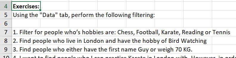
Filter the items to show the 5 most expensive:

Remove this filter, and instead show all of the expenses incurred in May but
paid in June:

Save this
workbook as Impressive filtering, then close it down.

You can unzip
this file to see the answers to this exercise, although please remember this is for your personal use only.

ПРАКТИЧЕСКАЯ РАБОТА № 7

Тема: Сортировка и фильтрация данных в Excel

Цель: приобрести практические навыки в работе с сортировкой и фильтрацией в программе Ms Excel 2007

Необходимо выполнить 3 практических задания входе работы.

1)Задание к практической работе:

Сортировка списков

1.Наберите таблицу в соответствии с рисунком 1

2.Выделите его.

3.Нажмите кнопку «Сортировка и фильтр» на анели «Редактирование» ленты «Главная».

4.Выберите «Сортировка от А до Я». Наш список будет отсортирован по первому столбцу, т.е. по полю ФИО.

5.Если надо отсортировать список по нескольким полям, то для этого предназначен пункт «Настраиваемая сортировка..». Сложная сортировка подразумевает упорядочение данных по нескольким полям. Добавлять поля можно при помощи кнопки «Добавить уровень».Рис3,4

Рис.3

Рис.4.

6.В итоге список будет отсортирован, согласно установленным параметрам сложной сортировки(рис. 5)

Рис.5.

7.Если надо отсортировать поле нестандартным способом, то для этого предназначен пункт меню»Настраиваемый список..» выпадающего списка «Порядок».

Перемещать уровни сортировки можно при помощи кнопок «Вверх» и «Вниз».

Не следует забывать и о контекстном меню. Из него, также, можно настроить сортировку списка. К тому же есть такие интересные варианты сортировки, связанные с выделением того или иного элемента таблицы.

Фильтрация списков

Краткая справка:

Основное отличие фильтра от упорядочивания — это то, что во время фильтрации записи, не удовлетворяющие условиям отбора, временно скрываются (но не удаляются), в то время, как при сортировке показываются все записи списка, меняется лишь их порядок.

Фильтры бывают двух типов: обычный фильтр (его еще называют автофильтр) и расширенный фильтр. Для применения автофильтра нажмите ту же кнопку, что и при сортировке — «Сортировка и фильтр» и выберите пункт «Фильтр» (конечно же, перед этим должен быть выделен диапазон ячеек).

В столбцах списка появятся кнопки со стрелочками, нажав на которые можно настроить параметры фильтра.

Поля, по которым установлен фильтр, отображаются со значком воронки. Если подвести указатель мыши к такой воронке, то будет показано условие фильтрации.

Для формирования более сложных условий отбора предназначен пункт «Текстовые фильтры» или»Числовые фильтры». В окне «Пользовательский автофильтр» необходимо настроить окончательные условия фильтрации.

При использовании расширенного фильтра критерии отбора задаются на рабочем листе.

Фильтры.2) Задание к практической работе:

1.Скопируйте и вставьте на свободное место шапку списка.

В соответствующем поле (полях) задайте критерии фильтрации.

2.Выделите основной список.

3.Нажмите кнопку «Фильтр» на панели «Сортировка и фильтр» ленты «Данные».

4.На той же панели нажмите кнопку «Дополнительно».

5.В появившемся окне «Расширенный фильтр» задайте необходимые диапазоны ячеек.

7.В результате отфильтрованные данные появятся в новом списке.

8.Расширенный фильтр удобно использовать в случаях, когда результат отбора желательно поместить отдельно от основного списка.

3)Задания к практической работе:

Самостоятельно выполните по созданной выше таблице:

А) С помощью фильтра выведите фамилии тех рабочих, оклад которых не превышает 12000 руб.

Б) С помощью расширенного фильтра выведите фамилии тех людей, которые работают в бухгалтерии

Г) Отсортируйте список по убыванию.

Лабораторно-практическая
работа № 11
«MS Excel 2007. Фильтрация (выборка) данных из списка»

Выполнив задания этой темы, вы научитесь:

·        
Выполнять
операции по фильтрации данных по определенному условию;

·        
Различать
операции по сортировке и фильтрации.

Фильтрация (выборка) данных в таблице
позволяет отображать только те строки, содержимое ячеек которых отвечает
заданному условию или нескольким условиям. В отличие от сортировки данные при
фильтрации не переупорядочиваются, а лишь скрываются те записи, которые не
отвечают заданным критериям выборки.

Фильтрация данных может выполняться двумя способами: с
помощью автофильтра или расширенного фильтра.

Для использования автофильтра нужно:

o    установить
курсор внутри таблицы;

o    выбрать
команду Данные — Фильтр — Автофильтр;

o    раскрыть
список столбца, по которому будет производиться выборка;

o    выбрать
значение или условие и задать критерий выборки в диалоговом окне Пользовательский
автофильтр.

Для восстановления всех строк исходной таблицы нужно
выбрать строку все в раскрывающемся списке фильтра или выбрать команду
Данные — Фильтр — Отобразить все.

Для отмены режима фильтрации нужно установить курсор
внутри таблицы и повторно выбрать команду меню Данные — Фильтр — Автофильтр
(снять флажок).

Расширенный фильтр позволяет формировать множественные
критерии выборки и осуществлять более сложную фильтрацию данных электронной
таблицы с заданием набора условий отбора по нескольким столбцам. Фильтрация
записей с использованием расширенного фильтра выполняется с помощью команды меню
Данные — Фильтр — Расширенный фильтр.

Задание.

Создайте таблицу в соответствие с образцом, приведенным
на рисунке. Сохраните ее под именем Sort.xls.

Технология выполнения
задания:

1.             
Откройте
документ Sort.xls

2.             
Установите
курсор-рамку внутри таблицы данных.

3.             
Выполните
команду меню Данные — Сортировка.

4.             
Выберите
первый ключ сортировки: в раскрывающемся списке «сортировать»
выберите «Отдел» и установите переключатель в положение «По
возрастанию» (Все отделы в таблице расположатся по алфавиту).

5.             
Если
же хотите, чтобы внутри отдела товары расположились по алфавиту, то выберите
второй ключ сортировки в раскрывающемся списке «Затем» выберите
«Наименование товара» и установите переключатель в положение «По
возрастанию».

Вспомним,что
нам ежедневно нужно распечатывать список товаров, оставшихся в магазине
(имеющих ненулвой остаток), но для этого сначала нужно получить такой список,
т.е. отфильтровать данные.

6.             
Установите
курсор-рамку внутри таблицы данных.

7.             
Выполните
команду меню Данные — Фильтр — Автофильтр.

8.             
Снимите
выделение в таблицы.

9.             
У
каждой ячейки заголовка таблицы появилась кнопка «Стрелка вниз», она
не выводится на печать, позволяющая задать критерий фильтра. Мы хотим оставить
все записи с ненулевым остатком.

10.          
Щелкните
по кнопке со стрелкой, появившейся в столбце Количество остатка.
Раскроется список, по которому будет производиться выборка. Выберите строку Условие.
Задайте условие: > 0. Нажмите ОК. Данные в таблице будут
отфильтрованы.

11.          
Вместо
полного списка товаров, мы получим список проданных на сегодняшний день
товаров.

12.          
Фильтр
можно усилить. Если дополнительно выбрать какой-нибудь отдел, то можно получить
список неподанных товаров по отделу.

13.          
Для
того, чтобы снова увидеть перечень всех непроданных товаров по всем отделам,
нужно в списке «Отдел» выбрать критерий «Все».

14.          
Можно
временно скрыть остальные столбцы, для этого, выделите столбец «№», и
в контекстном меню выберите Скрыть . Таким же образом скройте остальные
столбцы, связанные с приходом, расходом и суммой остатка. Вместо команды
контекстного меню можно воспользоваться командой Формат — Столбец — Скрыть.

15.          
Чтобы
не запутаться в своих отчетах, вставьте дату, которая будет автоматически
меняться в соответствии с системным временем компьютера Вставка — Функция —
Дата и время — Сегодня.

16.          
Как
вернуть скрытые столбцы? Проще всего выделить таблицу всю целиком, щелкнув по
пустой кнопке и выполнить команду Формат — Столбец — Показать.

17.          
Восстановите
исходный вариант таблицы и отмените режим фильтрации. Для этого щелкните по
кнопке со стрелкой и в раскрывшемся списке выберите строку Все, либо выполните
команду Данные — Фильтр — Отобразить все.

Источник: Ефимова О.В., Моисеева М.В., Шафрин Ю.А. Практикум по
компьтерной технологии. Упражнения, примеры, задачи. М.: АБФ, 1997

Проверочная тестовая работа

1.  Дана электронная таблица:
В ячейку D1 введена формула, вычисляющая выражение по формуле=(A2+B1-C1).

	A	B	C	D
1	1	3	4
2	4	2	5
3	3	1	2

1)  1     2)  2     3)  3
    4)  4

2.  Значение в ячейке С3 электронной таблицы

	A	B	C
1	3	9	=В2+$1
2	7	15	3
3	45	4	=C1-C2

1)  27     2) 5     3)  34
    4)  27

3.  Значение С6 электронной таблицы

	A	B	C
1	3	3	=СУММ(В2:С3)
2	0	2	6
3	=СТЕПЕНЬ(А5;2)	5	3
4	6	=МАКС(В1:В3)	7
5	5	4	35
6			=А3/В4+С1

<BR

равно

1)  22     2) 39     3)  26
    4)  21

4.  Дана электронная таблица:
Значение в ячейке С1 заменили на 7. В результате этого значение в ячейке D1
автоматически изменилось на 11.

	A	B	C	D
1	3	4	8
2	3	2	5
3	7	1	2

1)  записана формула В1+С1
2)  при любом изменении таблицы значение увеличивается на 3
3)  записана формула СУММ(А1:С1)
4)  записана формула СУММ(А1:А3)

5. Дан фрагмент электронной таблицы:
Значение ячейки С1 вычисляется по формуле =В1+$1

	A	B	C
1	3	2	5
2	7	1
3	4	4

1)  10     2) 6     3)  7
    4)  8

One of the most useful tools you have in Excel is the Filter tool.

You know that the filter is ON when you see arrows on the header of your table.

Activate the Filter

1. Select one of the cells of your table

2. Activate the filter in the Data > Filter

3. Now you see arrows in the header of your table

Display only a few rows

With the filter you can easily reduce the number of rows visible by selecting only one criterion.

Select one criterion (Filter on one column)

For instance, you might want to select only the rows in the beverages category.

1. Click on the arrow containing your criterion (here the column Category)
2. Uncheck all items (Select All)
3. Select only the item you want (in this case, Beverages)

Only the row containing this criterion is visible but the other rows are not deleted.

Rows are not deleted

When you activate the filter, you can hide the rows not equal to your filter.

As you can see, only the row numbers of the rows containing your filter are visible.

Moreover, the row numbers are blue. This indicates that a filter is active on your table.

Select multiple criteria (Filter on many columns)

You can select as many columns as you want.

For instance, if you want to select men from Germany (DE) and Austria (AT) who have bought from the Grocery category, you can do it like this:

How many rows are returned in your filter

When you activate a filter, you can see how many rows are returned by looking at the bottom left in the status bar

Remove the filter

There are many ways to remove a filter.

You can select the columns one by one and clear the filter for each one by clicking on the arrow and choosing Clear Filter From «Column Name», as illustrated here.

You can also remove all the filters at once with the option Data > Clear

Explanation

Advanced Filter allows us to quickly filter based on several criteria that are predefined in a separate table.

Advantages of Advanced Filter over “normal” filter:

• No need to choose each item we want to filter (imagine wanting to filter for 100 values out of 1,000), we can create a table instead.
• Allows us to filter based on several columns at once, using “AND” & “OR” operators.
  • AND – all conditions have to be met
  • OR  – At least one condition has to be met

Click here to download our absolutely FREE Advanced Filter exercise!

Advanced Filter example

In the table below, we would like to filter for people who live in London, Manchester, Glasgow or Cardiff:

Of course, you can manually tick the 4 cities, but what if you had to filter for 50 cities?

Let’s use Advanced Filter to do this!

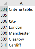
First step – We will create a table with one column, where we will list the cities for which we wish to filter. Above that list we will put a header.
Important: For Advanced Filter to work, we have to give our new column the same header as in the table we are filtering, for our example that will be “City”:

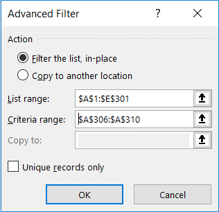
Second step – We will go the the “Data” ribbon and click on “Advanced”

Third step – We will now select the ranges for our list range (the range we want to filter) and criteria range (the table we created in the first step):

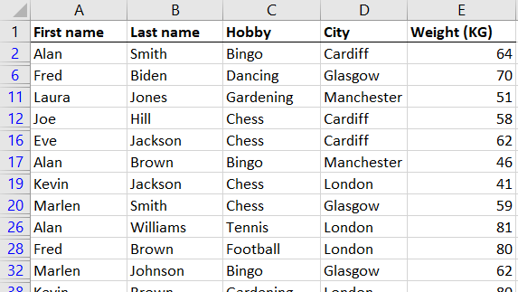
Success! Your table should now look like this:

To un-filter, simply click on “Clear” in the “Data” Ribbon:

And now let’s see it in action:

Advanced Filter with multiple columns

Besides filtering for multiple values, we can also use Advanced Filter to filter using several columns.

Filtering using AND logic:

This filter is useful when we want all the criteria to be met, for example:
We want to find all the people who are named Alan and like chess. How will we do this?

Answer: we’ll create a table that uses “AND” by putting all the criteria values in the same row.

 

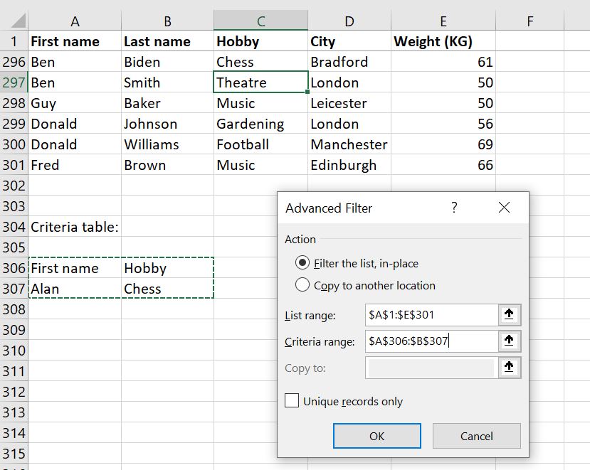
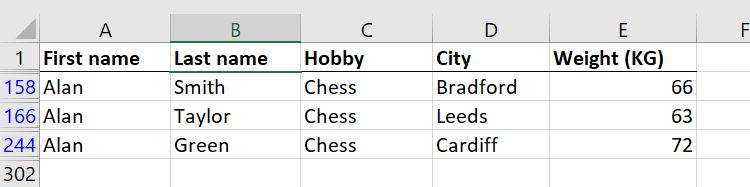
We asked the Advanced Filter to show us all the people who are named Alan AND like Chess. We did that by putting all the criteria in one row and using headers that match the original table.

And here’s the final result:

Filtering using OR logic:

This filter is useful when we want at least one of the criteria to be met, for example:
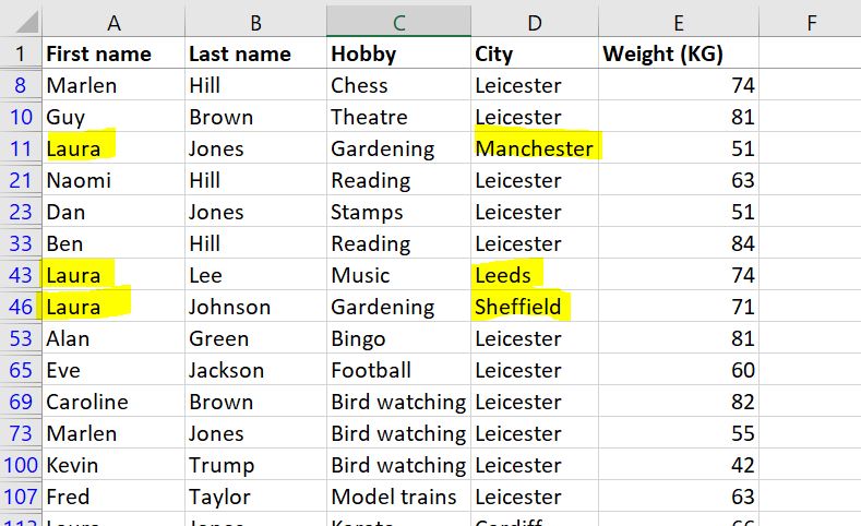
We want to find all the people who are either named Laura OR live in Leicester. How will we do this?

Answer: we’ll create a table that uses “OR” by putting all the criteria values in separate rows:

We asked the advanced Filter to show us all the people who are either named Laura OR live in Leicester (or both!). We did that by putting all the criteria in separate rows and using headers that match the original table.

Here’s the result:

Filtering numerical values using Advanced Filter

We can use Advanced Filter when we want to filter for all numerical values which are larger/smaller than a specific value.

We would follow the same steps as in previous examples, except in the criteria we will add “<“ or “>”.

And the result will be:

Tip – You can also use these operators:

<> – Does not equal to…
>= – Equals to or larger than…
<= – Equals to or smaller than…

Using wildcards in Advanced Filter

Excel Wildcards can be extremely useful when filtering complex tables.

We can use the “?” and “*” wildcards combined with Advanced Filter to do magics!

The ? (Question mark) wildcard

When we use “?” wildcard, Excel knows we want it to guess ONE character.
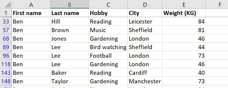
For example, if we look for the first name “B?n”, it will return a list filtered for first names that have the sequence b?n within them:

The result will be:

The * (Asterisk) wildcard

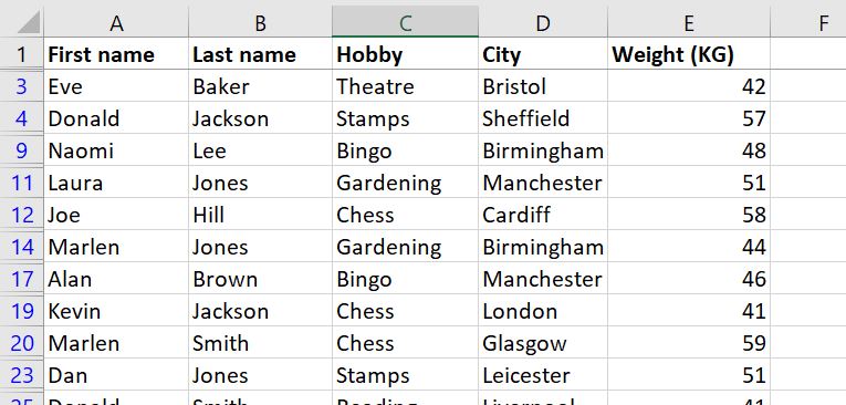
When we use “*”, Excel understands that we want it to guess an unknown number of characters – Anything between zero or more characters.
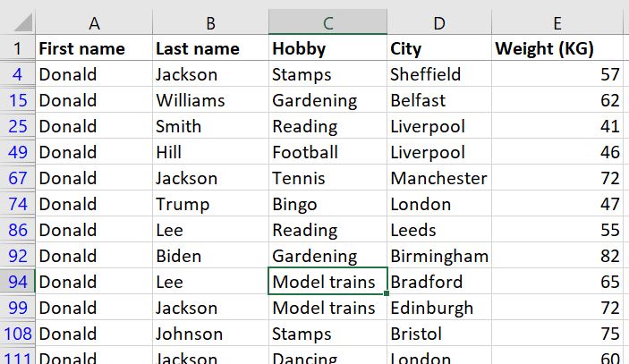
For example, if we look for the First Name “D*d” it will return a list filtered for first names that have the sequence “D*d” in them:

And the result:

Creating a new table from the filtered range

We learned how to filter a table, but what if we want to create a new table from the filtered data?
Simply click “Copy to another location” and mention where you want to have the new table in the “Copy to” field:

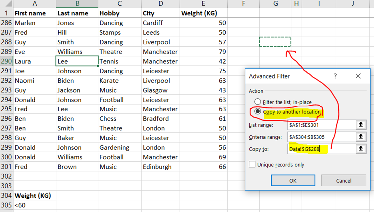
Warning – When you copy the filtered list to another location, you can’t undo (ctrl+z)

Now, time to practice Advanced Filter in Excel!

Click here to download the Advanced Filter Exercise – Which includes basic filtering, and/or filtering, wildcards and more. All exercises include solutions!  

Download the Advanced Filter exercise now!   

Федеральное агентство по образованию рф

Новосибирский
Государственный Университет
экономики
и управления

Кафедра
Экономической информатики

БОРИДЬКО
О.Н.

Методические
указания по выполнению
лабораторной
работы

«Фильтрация
в Microsoft Excel 2007,функции базы данных»

по
дисциплине «Информатика»

для
студентов 1 курса дневного
отделения
экономических специальностей

Новосибирск

2009

Табличный
процессор Microsoft
Excel 2007

Методические
указания к выполнению
лабораторной
работы № 3

”Фильтрация
в Excel,функции
базы данных”

1СПИСКИ
данных в EXCEL 3

2Фильтрация
данных в EXCEL 3

2.1Типы
критериев 3

2.1.1Критерии
на основе сравнения 4

2.1.2Критерии
в виде образца-шаблона 5

2.1.3Множественные
критерии на основе логических операций 5

2.1.4Вычисляемые
критерии на основе логических формул 5

3Средства
фильтрации 6

3.1Автофильтр 6

3.2Расширенный
фильтр 9

13

4ВСТРОЕННЫЕ
ФУНКЦИИ базы данных 15

5Вопросы
к защите лабораторной работы 18

1. СПИСКИ данных в
   EXCEL

При
работе с таблицами большую помощь могут
оказать содержащиеся в Excel
средства работы с базой данных.

Таблица
в Excel
представляет собой однотабличную
базу
данных.

В
Excel
базы данных называются списками.

Список
– определенным образом сформированный
на рабочем листе Excel
массив данных со столбцами и строками.

Список
может использоваться как база данных,
в которой строки выступают в качестве
записей,
а столбцы являются полями.
Первая строка списка при этом содержит
названия столбцов. Список должен быть
организован так, чтобы в каждом столбце
содержалась однотипная информация.
Пустые ячейки недопустимы.

1. Фильтрация данных в excel

Фильтрация
данных – это наиболее частые действия,
производимые со списком или базой
данных. Фильтрация
производится
на основе задаваемых пользователем
критериев
–
требований, налагаемых на информацию.
Результатом фильтрации является
временное скрытие записей, не
удовлетворяющих заданным критериям.

Для
фильтрации списков в Excel
существует две команды :

• Автофильтр

• Расширенный
  фильтр

Автофильтр
обеспечивает
простой и быстрый способ скрытия лишних
записей, оставляя на экране только те,
что удовлетворяют критериям.

Расширенный
фильтр
позволяет накладывать более сложные
условия отбора, которые могут включать
вычисляемые критерии.

1. Типы критериев

Чтобы
отфильтровать данные, необходимо прежде
всего описать то, что необходимо найти,
другими словами, задать диапазон
критериев.
Принципы составления диапазона
одинаковы и для автофильтра, и для
расширенного фильтра, хотя записываются
они в различных местах. Excel
поддерживает несколько типов критериев,
приведем основные из них:

• Критерии
  на основе сравнения
  – позволяют
  находить точные соответствия с помощью
  гибкого набора операций сравнения;

• Критерии
  в виде образца-шаблона
  – позволяют
  находить данные по соответствию
  некоторому шаблону (применяется только
  к тексту, либо к числам, отформатированным
  как текст);

• Множественные
  критерии на основе логических операций
  –
  позволяют объединить несколько критериев
  с помощью логических операций;

• Вычисляемые
  критерии на основе логических формул
  – позволяют
  создавать условия отбора, зависящие
  от значений логических формул.

Соседние файлы в предмете [НЕСОРТИРОВАННОЕ]

• #
• #
• #
• #
• #
• #
• #
• #
• #
• #
• #

Цель работы: научиться форматировать
данные в Microsoft Excel; ознакомится с понятиями
фильтрация, автофильтр, сортировка; научиться
использовать формулы в Microsoft Excel 2007.

Задание: Создайте таблицу в
соответствие с образцом, приведенным на рис. 1.

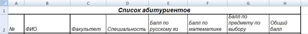
Рисунок 1. Образец таблицы

Выполнение:

Создайте новую книгу и сохраните ее под
названием Фильтрация. Откройте Лист 1 и
переименуйте его в Фильтр (ПКМ на Лист 1 ––>
Переименовать).
Отформатируйте лист Фильтр в соответствии с
требованиями:

– Объедините диапазон ячеек А1:G1 и введите
заголовок Список абитуриентов (шрифт – Arial, кегль
– 14, начертание – полужирное).
– В ячейки диапазона А2:Н2 введите заголовки
строк (шрифт – Arial, кегль – 12).
– В диапазон ячеек А3:А15 введите номер по порядку,
используя функцию протягивания.
– Установите границы для Заголовков.
– С помощью формы ввода (рис. 2) заполните
диапазон В3:G15. Выделите ячейки В2:G2 выберите пункт
меню Данные ––> Форма.

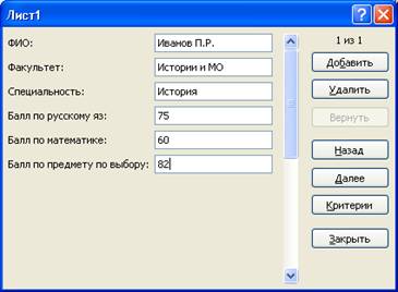
Рисунок 2. Форма ввода

Заполните таблицу 10-15 значениями.
В ячейке Н3 посчитайте сумму баллов за три
экзамена: =СУММ(E3:G3). Протяните эту формулу на
весь диапазон H3:H15. Задайте фон столбцам таблицы
(рис. 3).

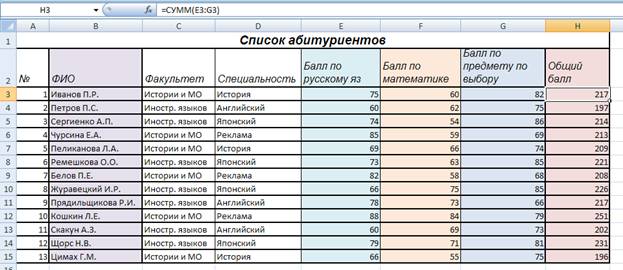
Рисунок 3. Оформление листа

Установите курсор-рамку внутри таблицы данных.
Выполните команду меню Данные ––>
Сортировка.
Выберите первый ключ сортировки: в
раскрывающемся списке «сортировать»
выберите Факультет и установите переключатель в
положение «По возрастанию» (Все факультеты в
таблице расположатся по алфавиту).
Если же хотите, чтобы внутри отдела
Специальности расположились по алфавиту, то
выберите второй ключ сортировки в
раскрывающемся списке «Затем» выберите
Специальность и установите переключатель в
положение «По возрастанию» (рис. 4).

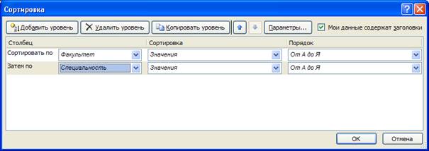
Рисунок 4. Сортировка записей

Затем необходимо отфильтровать данные.
Установите курсор-рамку внутри таблицы данных.
Выполните команду меню Данные ––> Фильтр
––> Автофильтр. Снимите выделение в
таблицы. Результат выполнение операции
представлен на рис. 5.

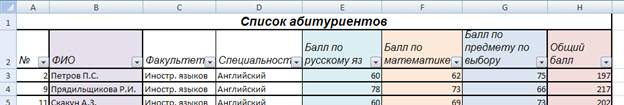
Рисунок 5. Применение автофильтра

У каждой ячейки заголовка таблицы появилась
кнопка «Стрелка вниз», она не выводится на
печать, позволяющая задать критерий фильтра.
Допустим, нам необходимы все записи, где Общий
балл будет больше 210.
Щелкните по кнопке со стрелкой, появившейся в
столбце Общий балл. Раскроется список,
по которому будет производиться выборка.
Выберите строку Условие. Задайте
условие: > 210. Нажмите ОК. Данные в
таблице будут отфильтрованы (рис. 6).

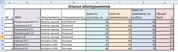
Рисунок 6. Результат применения фильтра

Вместо полного списка абитуриентов, мы получим
список набравших более 210 баллов. Фильтр можно
усилить. Если дополнительно выбрать какой-нибудь
факультет, то можно получить список абитуриентов
по факультету, набравших более 210 баллов.
Для того, чтобы снова увидеть перечень всех
абитуриентов, нужно в списке Факультет выбрать
критерий Все.
Можно временно скрыть остальные столбцы, для
этого, выделите столбец «№», и в контекстном
меню выберите Скрыть. Таким же образом
скройте остальные столбцы, связанные с баллами
по предметам. Вместо команды контекстного меню
можно воспользоваться командой Формат ––>
Столбец ––> Скрыть.
Чтобы не запутаться в своих отчетах, вставьте
дату в ячейку Н1, которая будет автоматически
меняться в соответствии с системным временем
компьютера Вставка ––> Функция ––> Дата
и время ––> Сегодня (рис. 7).

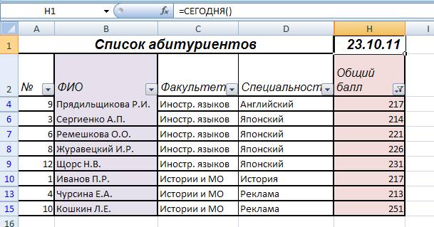
Рисунок 7. Добавления функции СЕГОДНЯ()

Для того чтобы вернуть скрытые столбцы
необходимо выделить таблицу всю целиком, щелкнув
по пустой кнопке и выполнить команду Формат
––> Столбец ––> Показать.
Восстановите исходный вариант таблицы и
отмените режим фильтрации. Для этого щелкните по
кнопке со стрелкой и в раскрывшемся списке
выберите строку Все, либо выполните команду
Данные ––> Фильтр ––> Отобразить все.

Контрольные вопросы:

1. Как создать новую книгу?
2. Каким образом можно переименовать лист?
3. Что такое форматирование документа?
4. Как изменить гарнитуру, кегль, начертание,
выравнивание текста?
5. Каким образом можно задать фон ячейки, листа?
6. Что такое функция протягивания? Как ей
пользоваться?
7. Каким образом можно заполнить ячейки с помощью
формы?
8. Для чего используется функция СУММ()?
9. Что такое диапазон ячеек? Как определяется
адрес диапазона?
10. Как можно использовать сортировку в Microsoft Excel?
11. Что такое автофильтр?
12. Каким образом можно задать специальные
значения для фильтрации?
13. Для чего используется функция СЕГОДНЯ()?

Data Filters are a very powerful way of analysing tables of data in Excel. Put simply they are a way of reducing the table down to just the items you want to see based on the selections you choose.

For example a simple table like this one, may have several hundred or thousand rows of data. However there may be only a few lines you are interested in. For example you may be only interested in people under the age of 18 or sales amounts that are negative (indicating a refund) or only see sales of red Ferraris.

Turning on the Filters

In Office 2003 Turn on the filters by selecting any cell in your table (contiguous section of data) and selecting Data, Filter, Auto Filter from the menu. (Keystroke ALT D F F)

The arrows will show up as in the next picture.

In Office 2007 the filters are quite different. They are turned on differently and behave differently also.

Turn them on by selecting  any cell in the data table and clicking Data, then Filter. (Keystroke CTRL+SHIFT+L)

Turning off the filters in both versions is simply repeating the same clicks or keystrokes.

Filtering the data

Once you have the filters turned on you are able to reduce the visible cells by clicking the arrow for any column and then selecting from the available items.

In 2003 this looks like this:

Selecting Navy reduces the data set from, in this case, 79 items to 7. Note the blue row numbers. These indicate the filtering that has hidden the rows between. Some formulas only work with visible cells. And these hidden cells will now be excluded from those formulas.

SUBTOTAL for example is a formula that will sum only visible cells. Select the cell two cells below the bottom of the table under a value column (Sales) and then double click the SIGMA Sum icon on the toolbar.

Note how the resulting formula displays only the value of the visible cells, though it is evaluating all cells in the column of the table.

The same effect can be achieved in Office 2007. However the selection process is somewhat different.

When you select the arrow you are presented with a number of different options. The sort function is made available from this menu. The custom number and text filters are contextual and made available through a right arrow and secondary menu.

The filters based on the actual data in the column are now presented as check boxes with the default being they are all selected. You can turn off all the items you don’t want to see, or in this case you can turn off Select All and then turn on Navy.

Now Click OK and the resulting data set will display the same items – those sales where the car colour was Navy.

Unfortunately in Office 2007 double clicking the sigma function button won’t give you subtotals but just the normal SUM formula. However entering the SUBTOTAL formula in will get the same mathematical result as Excel 2003.

There is a lot more that can be done with filters. Next time we will look at using the custom text and number filters.

See my previous posts on this subject and similar subjects.

Office 2007 Excel Data Auto Filter

Using the Advanced Filter in Excel

Turning Excel Auto Filters on and off in VBA

Creating Subtotals in Excel

Using the Advanced Filter Function in Excel to locate unique records

Saving Autofilter Criteria