
Use Excel as your calculator
Instead of using a calculator, use Microsoft Excel to do the math!
You can enter simple formulas to add, divide, multiply, and subtract two or more numeric values. Or use the AutoSum feature to quickly total a series of values without entering them manually in a formula. After you create a formula, you can copy it into adjacent cells — no need to create the same formula over and over again.
Subtract in Excel

Multiply in Excel
Divide in Excel
Learn more about simple formulas
All formula entries begin with an equal sign (=). For simple formulas, simply type the equal sign followed by the numeric values that you want to calculate and the math operators that you want to use — the plus sign (+) to add, the minus sign (—) to subtract, the asterisk (*) to multiply, and the forward slash (/) to divide. Then, press ENTER, and Excel instantly calculates and displays the result of the formula.
For example, when you type =12.99+16.99 in cell C5 and press ENTER, Excel calculates the result and displays 29.98 in that cell.
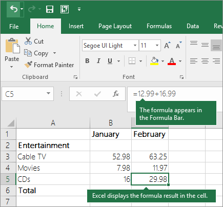
The formula that you enter in a cell remains visible in the formula bar, and you can see it whenever that cell is selected.
Important: Although there is a SUM function, there is no SUBTRACT function. Instead, use the minus (-) operator in a formula; for example, =8-3+2-4+12. Or, you can use a minus sign to convert a number to its negative value in the SUM function; for example, the formula =SUM(12,5,-3,8,-4) uses the SUM function to add 12, 5, subtract 3, add 8, and subtract 4, in that order.
Use AutoSum
The easiest way to add a SUM formula to your worksheet is to use AutoSum. Select an empty cell directly above or below the range that you want to sum, and on the Home or Formula tabs of the ribbon, click AutoSum > Sum. AutoSum will automatically sense the range to be summed and build the formula for you. This also works horizontally if you select a cell to the left or right of the range that you need to sum.
Note: AutoSum does not work on non-contiguous ranges.
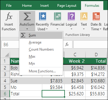
AutoSum vertically
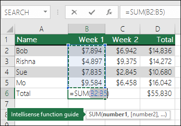
In the figure above, the AutoSum feature is seen to automatically detect cells B2:B5 as the range to sum. All you need to do is press ENTER to confirm it. If you need to add/exclude more cells, you can hold the Shift Key + the arrow key of your choice until your selection matches what you want. Then press Enter to complete the task.
Intellisense function guide: the SUM(number1,[number2], …) floating tag beneath the function is its Intellisense guide. If you click the SUM or function name, it will change o a blue hyperlink to the Help topic for that function. If you click the individual function elements, their representative pieces in the formula will be highlighted. In this case, only B2:B5 would be highlighted, since there is only one number reference in this formula. The Intellisense tag will appear for any function.
AutoSum horizontally

Learn more in the article on the SUM function.
Avoid rewriting the same formula
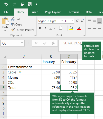
After you create a formula, you can copy it to other cells — no need to rewrite the same formula. You can either copy the formula, or use the fill handle  to copy the formula to adjacent cells.
For example, when you copy the formula in cell B6 to C6, the formula in that cell automatically changes to update to cell references in column C.
When you copy the formula, ensure that the cell references are correct. Cell references may change if they have relative references. For more information, see Copy and paste a formula to another cell or worksheet.
What can I use in a formula to mimic calculator keys?
|
Calculator key |
Excel method |
Description, example |
Result |
|
+ (Plus key) |
+ (plus) |
Use in a formula to add numbers. Example: =4+6+2 |
12 |
|
— (Minus key) |
— (minus) |
Use in a formula to subtract numbers or to signify a negative number. Example: =18-12 Example: =24*-5 (24 times negative 5) |
-120 |
|
x (Multiply key) |
* (asterisk; also called «star») |
Use in a formula to multiply numbers. Example: =8*3 |
24 |
|
÷ (Divide key) |
/ (forward slash) |
Use in a formula to divide one number by another. Example: =45/5 |
9 |
|
% (Percent key) |
% (percent) |
Use in a formula with * to multiply by a percent. Example: =15%*20 |
3 |
|
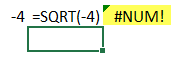
√ (square root) |
SQRT (function) |
Use the SQRT function in a formula to find the square root of a number. Example: =SQRT(64) |
8 |
|
1/x (reciprocal) |
=1/n |
Use =1/n in a formula, where n is the number you want to divide 1 by. Example: =1/8 |
0.125 |
Need more help?
You can always ask an expert in the Excel Tech Community or get support in the Answers community.
Need more help?
How to Calculate in Excel (Table of Contents)
- Introduction to Calculations in Excel
- Examples of Calculations in Excel
Introduction to Calculations in Excel
The following article provides an outline for Calculations in Excel. MS Excel is the most preferred option for calculation; most investment bankers and financial analysts use it to do data crunching, prepare presentations, or model data.
There are two ways to perform the Excel calculation: Formula and the second is Function. Where formula is the normal arithmetic operation like summation, multiplication, subtraction, etc. Function is the inbuilt formula like SUM (), COUNT (), COUNTA (), COUNTIF (), SQRT () etc.
Operator Precedence: It will use default order to calculate; if there is some operation in parentheses, then it will calculate that part first, then multiplication or division after that addition or subtraction. It is the same as the BODMAS rule.
Examples of Calculations in Excel
Here are some examples of How to Use Excel to Calculate Basic calculations.
You can download this Calculations Excel Template here – Calculations Excel Template
Example #1 – Basic Calculations like Multiplication, Summation, Subtraction, and Square Root
Here we are going to learn how to do basic calculations like multiplication, summation, subtraction, and square root in Excel.
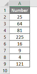
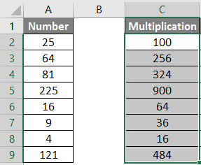
Let’s assume a user wants to perform calculations like multiplication, summation, subtraction by 4 and find out the square root of all numbers in Excel.
Let’s see how we can do this with the help of calculations.
Step 1: Open an Excel sheet. Go to sheet 1 and insert the data as shown below.
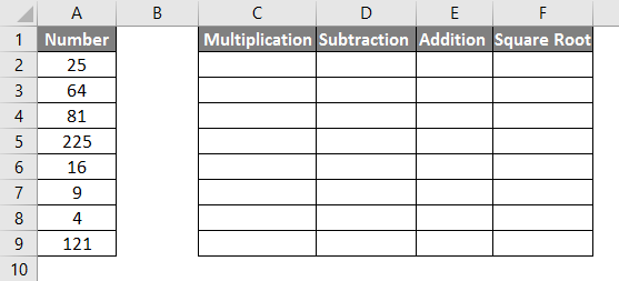
Step 2: Now create headers for Multiplication, Summation, Subtraction, and Square Root in row one.
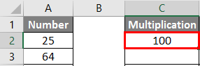
Step 3: Now calculate the multiplication by 4. Use the equal sign to calculate. Write in cell C2 and use asterisk symbol (*) to multiply “=A2*4“

Step 4: Now press on the Enter key; multiplication will be calculated.
Step 5: Drag the same formula to the C9 cell to apply to the remaining cells.
Step 6: Now calculate subtraction by 4. Use an equal sign to calculate. Write in cell D2 “=A2-4“
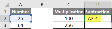
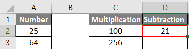
Step 7: Now click on the Enter key, the subtraction will be calculated.
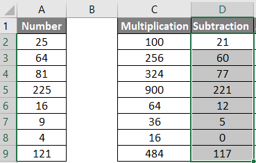
Step 8: Drag the same formula till cell D9 to apply to the remaining cells.
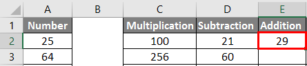
Step 9: Now calculate the addition by 4, use an equal sign to calculate. Write in E2 Cell “=A2+4“
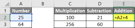
Step 10: Now press on the Enter key, the addition will be calculated.
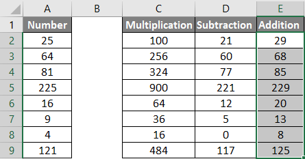
Step 11: Drag the same formula to the E9 cell to apply to the remaining cells.
Step 12: Now calculate the square root>> use equal sign to calculate >> Write in F2 Cell >> “=SQRT (A2“
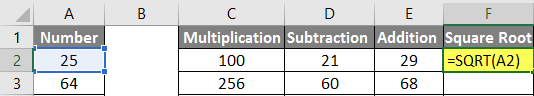
Step 13: Now, press on the Enter key >> square root will be calculated.
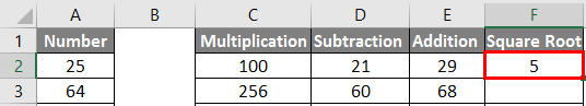
Step 14: Drag the same formula till the F9 cell to apply the remaining cell.
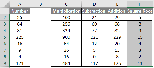
Summary of Example 1: As the user wants to perform calculations like multiplication, summation, subtraction by 4 and find out the square root of all numbers in MS Excel.
Example #2 – Basic Calculations like Summation, Average, and Counting
Here we are going to learn how to use Excel to calculate basic calculations like summation, average, and counting.
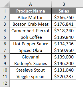
Let’s assume a user wants to find out total sales, average sales, and the total number of products available in his stock for sale.
Let’s see how we can do this with the help of calculations.
Step 1: Open an Excel sheet. Go to Sheet1 and insert the data as shown below.
Step 2: Now create headers for Result table, Grand Total, Number of Product and an Average Sale of his product in column D.
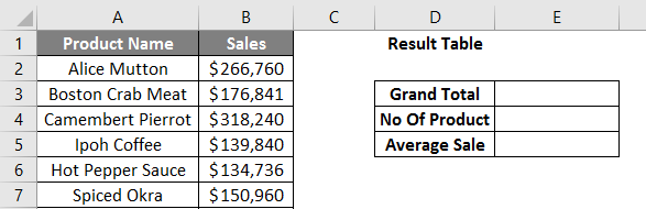
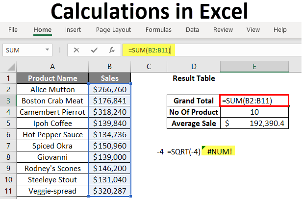
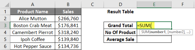
Step 3: Now calculate grand total sales. Use the SUM function to calculate the grand total. Write in cell E3. “=SUM (“
Step 4: Now, it will ask for the numbers, so give the data range, which is available in column B. Write in cell E3. “=SUM (B2:B11) “
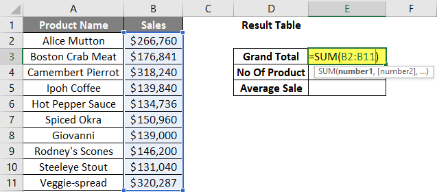
Step 5: Now press on the Enter key. Grand total sales will be calculated.
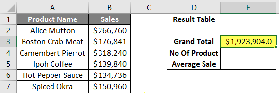
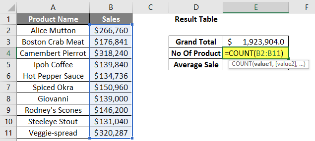
Step 6: Now calculate the total number of products in the stock, use the COUNT function to calculate the grand total. Write in cell E4 “=COUNT (“
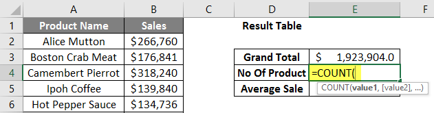
Step 7: Now, it will ask for the values, so give the data range, which is available in column B. Write in cell E4. “=COUNT (B2:B11) “
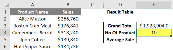
Step 8: Now press on the Enter key. The total number of products will be calculated.
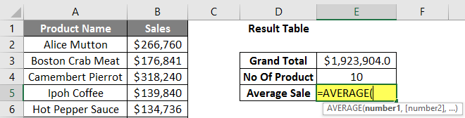
Step 9: Now calculate the average sale of products in the stock, use the AVERAGE function to calculate the average sale. Write in cell E5. “=AVERAGE (“
Step 10: Now, it will ask for the numbers, so give the data range which is available in column B. Write in cell E5. “=AVERAGE (B2:B11) “
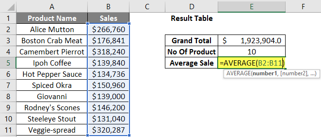
Step 11: Now click on the Enter key. The average sale of products will be calculated.
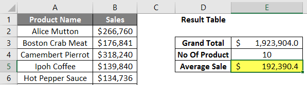
Summary of Example 2: As the user wants to find out total sales, average sales, and the total number of products available in his stock for sale.
Things to Remember about Calculations in Excel
- During calculations, if there are some operations in parentheses, then it will calculate that part first, then multiplication or division after that addition or subtraction.
- It is the same as the BODMAS rule: Parentheses, Exponents, Multiplication and Division, Addition and Subtraction.
- When a user uses an equal sign (=) in any cell, it means that the user is going to put some formula, not a value.
- A small difference from the normal mathematics symbol like multiplication uses asterisk symbol (*) and for division uses forward-slash (/).
- There is no need to write the same formula for each cell; once it is written, then just copy-paste to other cells, it will calculate automatically.
- A user can use the SQRT function to calculate the square root of any value; it has only one parameter. But a user cannot calculate square root for a negative number; it will throw an error #NUM!
- If a negative value occurs as output, use the ABS formula to determine the absolute value, which is an in-built function in MS Excel.
- A user can use the COUNTA in-built function if there is confusion in the data type because COUNT supports only numeric values.
Recommended Articles
This is a guide to Calculations in Excel. Here we discuss how to use excel to calculate along with examples and a downloadable excel template. You may also look at the following articles to learn more –
- Create a Lookup Table in Excel
- Use of COLUMNS Formula in Excel
- CHOOSE Formula in Excel with Examples
- What is Chart Wizard in Excel?
How to Use Excel as a Calculator?
In Excel, by default, there is no calculator button or option available in it. But, we can enable it manually from the “Options” section and then from the “Quick Access Toolbar,” where we can go to the commands not available in the ribbon. There further, we will find the calculator option available. Just click on “Add” and the “OK” to add the calculator to our Excel ribbon.
I have never seen beyond Excel to do the calculations in my career. Most of the calculations are possible with Excel spreadsheets. Not only are the calculations, but they are also flexible enough to reflect the immediate results if there are any modifications to the numbers, which is the power of applying formulas.
By using formulas, we need to worry about all the steps in the calculations because formulas will capture the numbers and show immediate real-time results for us. Excel has hundreds of built-in formulas to work with some of the complex calculations. On top of this, we see the spreadsheet as a mathematics calculator to add, divide, subtract, and multiply.
Table of contents
- How to Use Excel as a Calculator?
- How to Calculate in Excel Sheet?
- Example #1 – Use Formulas in Excel as a Calculator
- Example #2 – Use Cell References
- Example #3 – Cell Reference Formulas are Flexible
- Example #4 – Formula Cell is not Value, It is the only Formula
- Example #5 – Built-In Formulas are Best Suited for Excel
- Recommended Articles
- How to Calculate in Excel Sheet?
This article will show you how to use Excel as a calculator.
How to Calculate in Excel Sheet?
Below are examples of how to use Excel as a calculator.
You can download this Calculation in Excel Template here – Calculation in Excel Template
Example #1 – Use Formulas in Excel as a Calculator
As told, Excel has many of its built-in formulas, and on top of this, we can use Excel in the form of a calculator. To enter anything in the cell, we type the content in the required cell but apply the formula, and we need to start the equal sign in the cell.
Follow the below steps.
- So, to start any calculation, we need first to enter an equal sign, indicating that we are not just entering. Rather, we are entering the formula.

- Once the equal sign is entered in the cell, we can enter the formula. For example, assume that if we want to calculate the addition of two numbers, 50 and 30, we first need to enter the number we want to add.

- Once the number is entered, we need to go back to the basics of mathematics. Since we are doing the addition, we need to apply the PLUS (+) sign.

- After the addition sign (+), we must enter the second number. Then, we need to add to the first number.

- Now, press the ENTER key to get the result in cell A1.


So, 50 + 30 = 80.
It is the basic use of ExcelIn today’s corporate working and data management process, Microsoft Excel is a powerful tool.» Every employee is required to have this expertise. The primary uses of Excel are as follows: Data Analysis and Interpretation, Data Organizing and Restructuring, Data Filtering, Goal Seek Analysis, Interactive Charts and Graphs.
read more as a calculator. Similarly, we can use cell references to the formulaCell reference in excel is referring the other cells to a cell to use its values or properties. For instance, if we have data in cell A2 and want to use that in cell A1, use =A2 in cell A1, and this will copy the A2 value in A1.read more.
Example #2 – Use Cell References
For example, look at the below values in cells A1, A2, and A3.

- We must open an equal sign in the A4 cell.

- Then, select cell A1 first.

- After selecting cell A1, we need to put a plus sign and choose the A2 cell.

- Now, put one more plus sign and select A3 cell.
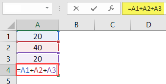
- Press the “ENTER” key to get the result in the A4 cell.
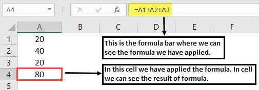
It is the result of using cell references.
Example #3 – Cell Reference Formulas are Flexible
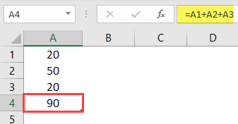
By using cell references, we can make the formula real-time and flexible. We said cell reference formulas are flexible because if we make any changes to the formula input cells (A1, A2, A3), it will reflect the changes in the formula cell (A4).
- We will change the number in cell A2 from 40 to 50.

We have changed the number but have not yet pressed the “ENTER” key. If we hit the “ENTER” key, we can see the result in the A4 cell.
- The moment we press the “ENTER” key, we see the impact on cell A4.
Example #4 – Formula Cell is not Value, It is the only Formula
We need to know when we use a cell reference for formulas because formula cells hold the result of the formula, not the value itself.
- Suppose we have a value of 50 in cell C2.

- If we copy and paste it to the next cell, we still get the value of 50 only.

- But, now come back to cell A4.

- Here we can see 90, but this is not the value but the formula. So we will copy and paste it to the next cell and see what we get.

Oh oh!!! We got zero.
We got zero because cell A4 has the formula =A1 + A2 + A3. When we copy cell A4 and paste it to B4, formula-referenced cells are changed from A1 + A2 + A3 to B1 + B2 + B3.
We got zero since there are no values in the cells B1, B2, and B3. So now, we will put 60 in any of the cells in B1, B2, and B3 and see the result.

- Look here the moment we have entered 60; we got the result as 60 because cell B4 already has the cell reference of the above three cells (B1, B2, and B3).

Example #5 – Built-In Formulas are Best Suited for Excel
We have seen how to use cell references for the formulas in the above examples. But those are best suited only for the small number of data sets, for a maximum of 5 to 10 cells.
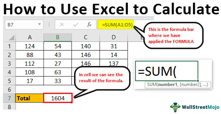
Now, look at the below data.

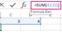
We have numbers from A1 to D5, and in the B7 cell, we need the total of these numbers. In these large data sets, we cannot give individual cell references, which takes a lot of time for us. That is where Excel’s built-in formulas come into the example.
- We should first open the SUM functionThe SUM function in excel adds the numerical values in a range of cells. Being categorized under the Math and Trigonometry function, it is entered by typing “=SUM” followed by the values to be summed. The values supplied to the function can be numbers, cell references or ranges.read more in cell B7.

- Now, hold the left-click of the mouse and select the range of cells from A1 to D5.

- After that, close the bracket and press the “Enter” key.

So, like this, we can use built-in formulas to work with large data sets.
This way, we can calculate in the Excel sheet.
Recommended Articles
This article is a guide to Excel as a Calculator. Here, we discuss how to do a calculation in an Excel sheet with examples and downloadable Excel templates. You may also look at these useful functions in Excel: –
- Calculate Percentage in Excel Formula
- Multiply in Excel Formula
- How to Divide using Excel Formulas?
- Excel Subtraction Formula
You may be familiar with Microsoft Excel. This application made by Microsoft Corporation is the application with the most users in the world in 140+ countries. This application has a myriad of Excel formulas that can accurately present numbers and data.
The primary function of Microsoft Excel is calculation, which is why it has been used by many users, both students and office workers. Despite other spreadsheet programs (competitors), Excel maintained its dominance and even became an industry standard.
Apparently, Excel seems too good to be true. All you have to do is enter an Excel formula, and almost everything you need to do manually can be done automatically. Use the best accounting software to do the cash flow forecast appropriately and analyze financial statements more optimally.
If you need to combine two sheets with the same data, Excel can do this. Do you need help with mathematics? Excel can do this. Are you using data from multiple cells? Excel can do this too.
In this article, you will understand the function of Excel in different professional fields. Then you’ll understand what formulas you need to know. Later, you will be able to apply automatic calculations to be used according to your needs.
Table Of Content
- The Uses of Excel in Professional Fields
- Complete Excel Formulas with Their Functions
- Conclusion
Also Read: 5 Common Bookkeeping Mistakes on Small Businesses
The Uses of Excel in Professional Fields
Many job openings require candidates to master Excel. Not surprisingly, excel is needed by a wide variety of fields of work that require data collection.
To that end, we will present the following professions, which can benefit from the use of Excel, among others:
Accountancy
It is widespread for accountants to be able to use Excel. The field of accounting benefits from using Microsoft Excel in several ways, including making it easier to calculate corporate profit and loss, identify large profits over a period, calculate employee salaries, and more.
An accountant can facilitate his work by using the accounting system as a tool he worked. The system can provide convenience in managing the company’s financial circulation and calculating it optimally and accurately.
Also Read: Salary Slip: Understanding, Benefits, Format, Example
Mathematical calculations
The next advantage of using Microsoft Excel is mathematical calculations. Use calculations to find data from numbers, subtractions, multiplications, and divisions, as well as various other variations such as calculating the slope.
Data processing
In data management, there are helpful excel formulas, including managing statistical databases, calculating data, searching for median values, and averages, and searching for the maximum and minimum values of data sets.
Graphic creation
Excel allows you to create graphics. Such as graphing population development data for one year, the graph of student library visits for one year, the student graduation graph for six years, the graph of student number development for three years, and others.
Table operations
The last application is to be able to operate the table. With a total of 1,084,576 rows and 16,384 columns in Microsoft Excel, it will make it easier for you to enter data that requires a large number of columns and rows.
Complete Excel Formulas with Their Functions
In addition to the functionality and use of Microsoft Excel mentioned earlier, operating this Excel program requires Excel formulas. Each formula has a different function that you can use for a specific need.
Here are the Excel formulas you need to know, among others:
| Formulas | Functional Description |
| SUM | Summing |
| AVERAGE | Looking for Average Values |
| AND | Finding Value by comparison and |
| NOT | Finding Value with Exceptions |
| OR | Finding Value by Comparison or |
| SINGLE IF | Looking for Values If Conditions ARE RIGHT/WRONG |
| MULTI IF | Finding Values If Conditions ARE RIGHT/WRONG With Many Comparisons |
| AREAS | View The Number of Areas (Range or Cells) |
| CHOOSE | View Selection Results Based on Index Numbers |
| HLOOKUP | Search for Data from a table organized in a horizontal format |
| VLOOKUP | Search for Data from a table arranged in an upright format |
| MATCH | Displays the position of a specific cell address |
| COUNTIF | Counting the Number of Cells in a Range with specific criteria |
| COUNTA | Counting the Number of Filled Cells |
| CEILING | Round the number up |
| FLOOR | Rounds numbers down |
| DAY | Looking for The Value of the Day |
| MONTH | Searching for the Value of the Moon |
| YEAR | Looking for Year Value |
| DATE | Get a Date Value |
| LOWER | Change text letters to lowercase |
| UPPER | Change Text Letters to UpperCase |
| PROPER | Change the Initial Character of the Text To UpperCase |
For more information about how to use the excel function formulas mentioned above, here is a detailed description, along with examples:
SUM
This Excel summation formula has the primary function of summing numbers in specific cells. However, it is also often used to complete a job or task quickly.
To use SUM, first create a summation table and enter the summation formula below. For example, =SUM(G8:H8), or as shown in the image below:
Then, if the SUM formula has been entered, press enters to specify the amount. As shown in the picture below:
AVERAGE
The primary function of the AVERAGE formula or the average formula in Excel is to find the average value of a variable. The trick is to create a table for grades and then enter the AVERAGE formula to determine the student’s grade point average. For example, =AVERAGE(D2:F2), as in the following image:
If you enter the AVERAGE formula, press enters to see the result, shown in the image below.
AND
The AND formula function generates a TRUE value if all previously tested arguments are correct or can return a FALSE value if all arguments or answers are incorrect.
To determine TRUE or FALSE, you must create a table and enter THE FORMULA AND. For example, =AND(G7>I7).
This technique is usually used to help fill out questionnaires or answer question columns to speed up the value-setting process.
NOT
The NOT formula has the opposite function of the AND formula because it produces TRUE if the condition tested is FALSE and FALSE if the condition tested is TRUE.
The first step is to create a table and enter the FORMULA NOT to find out the results. For example, as shown in the diagram below, =NOT(G7>J7).
OR
The OR is the following excel formula that will produce TRUE data if some given argument is correct. If all of the arguments presented are incorrect, the answer is FALSE.
A student’s average test score result is an example of how OR can use it in Excel. If it is less than 70, he must repeat the course; if it is greater than 70, the student graduates.
SINGLE IF
The IF function is to return a value that, when examined, is TRUE and another value that is visible as FALSE.
Not much different from the technique of using formulas in OR. It just seems more straightforward.
For example, when a student’s average grade is less than 75, that student does not graduate, and vice versa. How to create an IF formula is =IF(J8<75;” NOT GRADUATING”;” PASS”). To be clear, take a look at the following image:
After entering the formula, press enters, and the result will match what you ordered.
MULTI IF
This formula is a further lesson from SINGLE IF, but if SINGLE IF only uses only one condition with two options, The MULTI IF uses two terms and three options.
A Double/Multi FORMULA is a type of logic-IF formula consisting of 2 or more IF in formula writing. If a single IF only needs 1 IF, for example, =IF(B2=>=70;” Graduated”;” Failed”) then Double IF requires more than 1 IF, for example, =IF(B2>=70;” Good”;IF(B2>=50;” Enough”;” Less”)).
So that the full Excel formula will provide Syntax on Double / Multi IF, among others:
=IF(Logical_Test; Value_If_True;IF(Logical_Test; Value_If_True; Value_If_False))
AREAS
You can use the usability of AREAS if you want to calculate the number of areas you want to select. The AREAS formula can use the formula =AREAS(G6:K8).
The result is one area. The results are based on the example in the image of selecting only one range of cells.
CHOOSE
The primary function of a CHOOSE formula is to display selection results based on index numbers or sequences in reference (VALUE) that contain text, numeric, formula, or range names. The image below shows an example of how to write the CHOOSE formula.
Meanwhile, the results of the CHOOSE formula are shown in the image below.
HLOOKUP
The HLOOKUP function displays data from tables arranged horizontally. However, The arrangement of tables or data in the first row should be based on small to large sequences or raising them.
For example, the number 1,2,3,4… Or the letter A-Z. Sort by ascending the menu if you previously typed randomly. Cases like the ones listed below are examples.
=HLOOKUP(Cells that contain packet types; Range cell table details costs; The location of the data column you want to retrieve;0).
VLOOKUP
The primary function of the VLOOKUP formula is almost identical to the HLOOKUP formula; The difference is that the VLOOKUP formula displays data from tables arranged in an upright or vertical format. The requirement is that the first row of the data table is prepared in small to large order or up.
For example 1,2,3,4… Or the letter A-Z. For example 1,2,3,4… Or the letter A-Z. Sort through the Ascending menu if you previously typed randomly.
MATCH
The MATCH function is one of the components of an Excel formula that you can use to perform lookups or reference data searches.
The MATCH function works by finding the relative position of a value in a range or array and generating a number that is the index of the cell’s relative position that contains the value it is looking for.
The use of the Excel MATCH function must follow the syntax rules, namely MATCH(lookup_value, lookup_array, [match_type])
To better understand, understand the image below:
COUNTIF
COUNTIF is a helpful formula for counting the number of cells that have the same criteria. As a result, you no longer have to struggle with data sorting.
Assume you’re doing a survey. You want to know how many civil servants there are out of 20 respondents. As a result, you can use the following formulas:
To get started, all you need to do is enter the range of cells you want to identify into the COUNTIF formula (B2:B21)
Then, enter the cell calculation criteria, namely “PNS” (must be in quotation marks).
This formula produces a result of 7. So, out of 20 respondents, seven were civil servants.
COUNTA
COUNTA has the function of counting the number of cells that contain numbers and the number of cells that contain anything. As a result, you can determine the number of cells that are not empty.
Assume that cells A1 through D1 are words and cells G1 through I1 number. Therefore the use of the formula is =COUNTA(A1:I1)
That results in 7 because the empty cells are only E1 and F1.
CEILING
The CEILING formula can round the number UP at the multiple values of a specific number. The formula is CEILING (CELLS number; Multiples).
Misalnya, CEILING(G9;100). Then the number on Cells G9 will be rounded up with a multiple of 100.
FLOOR
If the previous use of the formula is to round to the nearest integer and above, the FLOOR formula is used to round to the nearest integer. The formula is almost identical to the one for CEILING, but with the addition of FLOOR.
The FLOOR formula is FLOOR (Number cell; Multiples).
DAY
The DAY formula is used to find the date type data’s day (in the numbers 1-31). Consider the DAY function (column B). The date data in column A will be extracted and converted into numbers 1-31, following the explanation through the image:
After entering the formula =DAY(NUMBER), press enters and see the results below:
MONTH
Almost similar to the DAY formula, the use of the MONTH formula to search for months (in numbers 1-12) from date type data. For example, the use of the MONTH function (column K) of a column I date data, after extracting it, produces the numbers 1-12 as in the figure below:
YEAR
Meanwhile, there is a YEAR formula. The way you use this formula is similar to the way the previous two formulas were. The use of the YEAR formula takes years (in the range of 1900-9999) from date-type data.
DATE
The DATE formula has a function that allows you to get date data types by entering years, months, and days. The DATE function is the opposite of the DAY, MONTH, and YEAR functions, which describe month and year-type data from their respective dates.
Year, month, and day data in the form of numbers combined with the DATE function generate data with data types, as shown in the figure below. Date formula writing image, namely:
LOWER
The lower formula function converts all uppercase letters in the text to lowercase. To use the formula, type the LOWER command, and texts will convert the desired writing to lowercase.
For example, when implementing the LOWER formula with the formula =LOWER (Don’t Forget to Use HashMicro Software), the result is “don’t forget to use has micro software.”
UPPER
In addition to lower formulas, Microsoft Excel includes upper formulas. The use of UPPER is to convert all text containing lowercase letters into uppercase, the opposite of the LOWER function.
For example, if you type UPPER (hashmicro), your writing will be entirely in capital letters.
PROPER
Sometimes you forget to write sentences in all lowercase letters and no capital letters. So with the PROPER formula, you can capitalize on the first character in each word while keeping the rest. The formula is APPROPRIATE (text).
Conclusion
Although understanding Excel entirely takes time, you will be familiar with all the correct formulas and applications.
In a company, the use of Excel is overwhelming, especially in presenting data, statistics, and company finances such as salaries. The digital world is bringing corporate transformation to provide information and payroll more easily with automated systems. You can use HashMicro accounting software as a tool to calculate financial circulation optimally and accurately.
Moreover, HashMicro has a system that helps with all your human resource and employee administration tasks. With HashMicro’s HRM Software, calculates salaries, and manages leave and attendance lists, reimbursement processes, timesheets, and other operational activities in just seconds.
Produce reports accurately and comprehensively like thousands of large companies that have joined HashMicro. To check out more, click here.
Ready solutions for Excel with the help of formulas working with data spans in the process of complex computations and calculations.
Computing operations with the help of formulas
 The Formula Bar in Excel, its settings and the purpose.
How to use the formula string and what advantages does it provide for entering and editing data in cells? How to enable or disable the formula bar in the program settings.
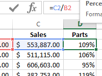 Percentage of the plan implementation by formula in Excel.
The examples of two formulas for calculating of percentages from numbers when analyzing the implementation of sales plans. The example, when and how to use the percentage format of cells.