
Excel for Microsoft 365 Excel for Microsoft 365 for Mac Excel for the web Excel 2021 Excel 2021 for Mac Excel 2019 Excel 2019 for Mac Excel 2016 Excel 2016 for Mac Excel 2013 Excel 2010 Excel 2007 Excel for Mac 2011 Excel Starter 2010 More…Less
You use the SUMIF function to sum the values in a range that meet criteria that you specify. For example, suppose that in a column that contains numbers, you want to sum only the values that are larger than 5. You can use the following formula: =SUMIF(B2:B25,»>5″)

This video is part of a training course called Add numbers in Excel.
Tips:
-
If you want, you can apply the criteria to one range and sum the corresponding values in a different range. For example, the formula =SUMIF(B2:B5, «John», C2:C5) sums only the values in the range C2:C5, where the corresponding cells in the range B2:B5 equal «John.»
-
To sum cells based on multiple criteria, see SUMIFS function.
Important: The SUMIF function returns incorrect results when you use it to match strings longer than 255 characters or to the string #VALUE!.
Syntax
SUMIF(range, criteria, [sum_range])
The SUMIF function syntax has the following arguments:
-
range Required. The range of cells that you want evaluated by criteria. Cells in each range must be numbers or names, arrays, or references that contain numbers. Blank and text values are ignored. The selected range may contain dates in standard Excel format (examples below).
-
criteria Required. The criteria in the form of a number, expression, a cell reference, text, or a function that defines which cells will be added. Wildcard characters can be included — a question mark (?) to match any single character, an asterisk (*) to match any sequence of characters. If you want to find an actual question mark or asterisk, type a tilde (~) preceding the character.
For example, criteria can be expressed as 32, «>32», B5, «3?», «apple*», «*~?», or TODAY().
Important: Any text criteria or any criteria that includes logical or mathematical symbols must be enclosed in double quotation marks («). If the criteria is numeric, double quotation marks are not required.
-
sum_range Optional. The actual cells to add, if you want to add cells other than those specified in the range argument. If the sum_range argument is omitted, Excel adds the cells that are specified in the range argument (the same cells to which the criteria is applied).
Sum_range
should be the same size and shape as range. If it isn’t, performance may suffer, and the formula will sum a range of cells that starts with the first cell in sum_range but has the same dimensions as range. For example:
range
sum_range
Actual summed cells
A1:A5
B1:B5
B1:B5
A1:A5
B1:K5
B1:B5
Examples
Example 1
Copy the example data in the following table, and paste it in cell A1 of a new Excel worksheet. For formulas to show results, select them, press F2, and then press Enter. If you need to, you can adjust the column widths to see all the data.
|
Property Value |
Commission |
Data |
|---|---|---|
|
$100,000 |
$7,000 |
$250,000 |
|
$200,000 |
$14,000 |
|
|
$300,000 |
$21,000 |
|
|
$400,000 |
$28,000 |
|
|
Formula |
Description |
Result |
|
=SUMIF(A2:A5,»>160000″,B2:B5) |
Sum of the commissions for property values over $160,000. |
$63,000 |
|
=SUMIF(A2:A5,»>160000″) |
Sum of the property values over $160,000. |
$900,000 |
|
=SUMIF(A2:A5,300000,B2:B5) |
Sum of the commissions for property values equal to $300,000. |
$21,000 |
|
=SUMIF(A2:A5,»>» & C2,B2:B5) |
Sum of the commissions for property values greater than the value in C2. |
$49,000 |
Example 2
Copy the example data in the following table, and paste it in cell A1 of a new Excel worksheet. For formulas to show results, select them, press F2, and then press Enter. If you need to, you can adjust the column widths to see all the data.
|
Category |
Food |
Sales |
|---|---|---|
|
Vegetables |
Tomatoes |
$2,300 |
|
Vegetables |
Celery |
$5,500 |
|
Fruits |
Oranges |
$800 |
|
Butter |
$400 |
|
|
Vegetables |
Carrots |
$4,200 |
|
Fruits |
Apples |
$1,200 |
|
Formula |
Description |
Result |
|
=SUMIF(A2:A7,»Fruits»,C2:C7) |
Sum of the sales of all foods in the «Fruits» category. |
$2,000 |
|
=SUMIF(A2:A7,»Vegetables»,C2:C7) |
Sum of the sales of all foods in the «Vegetables» category. |
$12,000 |
|
=SUMIF(B2:B7,»*es»,C2:C7) |
Sum of the sales of all foods that end in «es» (Tomatoes, Oranges, and Apples). |
$4,300 |
|
=SUMIF(A2:A7,»»,C2:C7) |
Sum of the sales of all foods that do not have a category specified. |
$400 |
Top of Page
Need more help?

See also
SUMIFS function
COUNTIF function
Sum values based on multiple conditions
How to avoid broken formulas
VLOOKUP function
Need more help?
Improve Article
Save Article
Like Article
Improve Article
Save Article
Like Article
Excel is a great tool to use in data collection and entry and nowadays it is widely used worldwide. To make the tasks of data management easier Excel has some built-in functions and formulas. SUMIF is such a function. This function easily sums the particular numbers in a large dataset. This is basically a worksheet function and comes under the Math & Trigonometry function.
This function does exactly what its name indicates. Using this function we can get the ‘SUM’ of numbers of a particular range ‘IF’ the given criteria is satisfied. This function actually evaluates the sum of a particular range applying a condition. And in this function, we can apply criteria to one range and sum up another range according to the criteria.
Syntax:
SUMIF(range, criteria, [sum_range](optional))
***[sum_range] is an optional argument.
This function accepts range, criteria(condition), and sum_range(optional argument) as its argument and returns the sum of the sum_range or the range according to the given arguments. The arguments are discussed below.
Arguments:
Arguments of the SUMIF function are the following:
- range(Required): This is the range of the cells that will be evaluated to check the given criteria or condition. These cells may contain numbers or names, dates(must be in standard excel formats), arrays, references(that contains numbers).
- criteria(Required): This argument is the criteria that need to be satisfied to add a cell of the given range. It can be a number, expression(logical or mathematical), text, reference, or a function. If the criteria is a mathematical or logical expression it must be written within double quote(Eg: ” >1000″). On the other hand, if the criteria is a number then the double quote is not required(Eg: 56). There are some special symbols like a question mark(‘?’) And asterisk(‘*’) with some special use:
- A question mark(?) can be used to match a single character.
- An asterisk(*) can be used to match a sequence of characters.
- And if we want to match a question mark(?) or an asterisk in the cell we need to use a tilde sign before them(Eg: “~?”).
- sum_range(Optional): This is the actual range that will be added cell by cell if the given criteria meet. But if this argument is not provided then the SUMIF function will return the sum of the range argument. sum_range should be of the same dimension of range argument for better performance.
Return Value:
This function sums the numbers in the given range and returns the numerical value of the sum.
Example:
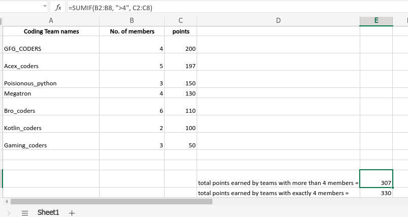
An Excel sheet has been taken as an example and the SUMIF function has been used in several formats.
| Coding Team names(Column A) | No. of members(Column B) | points(Column C) |
|---|---|---|
| GFG_CODERS | 4 | 200 |
| Acex_coders | 5 | 197 |
| Poisionous_python | 3 | 150 |
| Megatron | 4 | 130 |
| Bro_coders | 6 | 110 |
| Kotlin_coders | 2 | 100 |
| Gaming_coders | 3 | 50 |
Then we will apply the SUMIF() function to the above table:
| SUMIF() function | What the function does | Output result |
|---|---|---|
| =SUMIF(B2:B8, “>4”, C2:C8) | If the no. of members in column B is greater than 4 then add the corresponding points of column C. | 307 |
| =SUMIF(B2:B8, 4, C2:C8) | If the no. of members in column B is equal to 4 then add the corresponding points of column C. | 330 |
| =SUMIF(A2:A8, “GFG_CODERS”, C2:C8) | Search for “GFG_CODERS” in column A and add the corresponding points in column C. | 200 |
| =SUMIF(C2:C8, “>110”) | Here the sum_range argument is not provided. So it will check the cells of C column and if the points are greater than 110 add it to the result. | 677 |
| =SUMIF(A2:A8, “*rs”, C2:C8) | Here it will find the names of the teams ending with “rs” / “RS” in column A and add the corresponding points to the sum. | 657 |
Output:
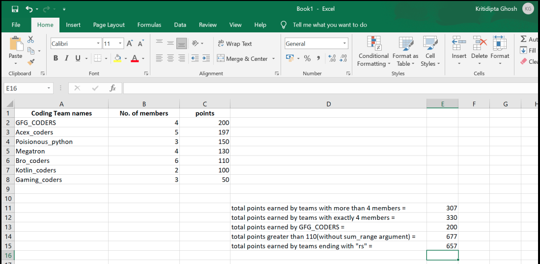
Output Excel Sheet
Using SUMIF function.
Like Article
Save Article
На чтение 2 мин
Функция СУММЕСЛИ (SUMIF) в Excel используется для суммирования значений, отвечающих заданным вами критериям.
Содержание
- Что возвращает функция
- Синтаксис
- Аргументы функции
- Дополнительная информация
- Примеры использования функции СУММЕСЛИ в Excel
Что возвращает функция
Возвращает сумму чисел, указанных в качестве аргументов и отвечающих заданным в формуле критериям.
 Больше лайфхаков в нашем Telegram Подписаться
Синтаксис
=SUMIF(range, criteria [sum_range]) — английская версия
=СУММЕСЛИ(диапазон; условие; [диапазон_суммирования]) — русская версия
Аргументы функции
- range (диапазон) — диапазон ячеек, по которым оцениваются критерии. Аргументом могут быть числа, текст, массивы или ссылки, содержащие числа;
- criteria (условие) — критерии, которые проверяются по указанному диапазону ячеек и определяют, какие ячейки суммировать;
- sum_range (диапазон_суммирования) — (не обязательно) суммируемые ячейки. Если этот аргумент не указан, то функция использует аргумент range (диапазон) в качестве sum_range (диапазон_суммирования).
Дополнительная информация
- суммирование ячеек в функции СУММЕСЛИ производится на основе одного критерия, если вам необходимо указать несколько критериев — используйте функцию SUMIFS (СУММЕСЛИМН);
- пустые и текстовые ячейки в аргументе sum_range (диапазон_суммирования) игнорируются;
- критерием для функции могут служить числа, выражения, результаты вычисления из других ячеек, текст или формула;
- если в качестве критерия указан текст или математический/логический символ (=,+,-,/,*), то такие значения должны быть указаны в двойных кавычках;
- аргумент с критерием не должен быть длиннее чем 255 символов;
- в качестве критерия могут использоваться подстановочные знаки (*);
- если количество ячеек в диапазоне критерия и аргументе sum_range (диапазон_суммирования) различаются, то размер диапазона критерия будет в приоритете.
Примеры использования функции СУММЕСЛИ в Excel
The SUMIF function sums cells in a range that meet a single condition, referred to as criteria. The SUMIF function is a common, widely used function in Excel, and can be used to sum cells based on dates, text values, and numbers. Note that SUMIF can only apply one condition. To sum cells using multiple criteria, see the SUMIFS function.
Syntax
The generic syntax for SUMIF looks like this:
=SUMIF(range,criteria,[sum_range])The SUMIF function takes three arguments. The first argument, range, is the range of cells to apply criteria to. The second argument, criteria, is the criteria to apply, along with any logical operators. The last argument, sum_range, is the range that should be summed. Note that sum_range is optional. If sum_range is not provided, SUMIF will sum cells in the first argument, range.
Examples: Basic Usage | Criteria in another cell | Not equal to | Blank cells | Dates | Wildcards | Videos
Applying criteria
The SUMIF function supports logical operators (>,<,<>,=) and wildcards (*,?) for partial matching. The tricky part about using the SUMIF function is the syntax needed to apply criteria. This is because SUMIF is in a group of eight functions that split logical criteria into two parts, range and criteria. Because of this design, operators need to be enclosed in double quotes («»). The table below shows examples of the syntax needed for common criteria:
| Target | Criteria |
|---|---|
| Cells greater than 75 | «>75» |
| Cells equal to 100 | 100 or «100» |
| Cells less than or equal to 100 | «<=100» |
| Cells equal to «Red» | «red» |
| Cells not equal to «Red» | «<>red» |
| Cells that are blank «» | «» |
| Cells that are not blank | «<>» |
| Cells that begin with «X» | «x*» |
| Cells less than A1 | «<«&A1 |
| Cells less than today | «<«&TODAY() |
Notice the last two examples involve concatenation with the ampersand (&) character. Any time you are using a value from another cell, or using the result of a formula in criteria with a logical operator like «<«, you will need to concatenate. This is because Excel needs to evaluate cell references and formulas to get a value before that value can be joined with an operator.
Limitations
There are a couple of limitations with SUMIF that you should be aware of. First, SUMIF only supports a single condition. If you need to sum cells using multiple criteria, use the SUMIFS function. Second, the SUMIF function requires an actual range for the range argument; you can’t substitute an array. This means you can’t do things like extract the year from a range that contains dates inside the SUMIF function. If you need to manipulate values that appear in the argument before applying criteria, the SUMPRODUCT function is a flexible solution.
Basic usage
With numbers in the range A1:A10, you can use SUMIF to sum cells greater than 5 like this:
=SUMIF(A1:A10,">5")If the range B1:B10 contains color names like «red», «blue», and «green», you can use SUMIF to sum numbers in A1:A10 when the color in B1:B10 is «red» like this:
=SUMIF(B1:B10,"red",A1:A10)Notice A1:A10 is now entered as the sum_range, because it is different from range, which contains only color names. To recap: criteria is applied to cells in range. When cells in range meet criteria, corresponding cells in sum_range are summed. The sum_range argument is optional. If sum_range is omitted, the cells in range are summed instead.
Worksheet example
In the worksheet shown, there are three SUMIF formulas. In the first formula (G5), SUMIF returns total Sales where Name = «jim». In the second formula (G6), SUMIF returns total Sales where State = «ca» (California). In the third formula (G7), SUMIF returns the total of Sales > 100:
=SUMIF(B5:B15,"jim",D5:D15) // name = "jim"
=SUMIF(C5:C15,"ca",D5:D15) // state = "ca"
=SUMIF(D5:D15,">100") // sales > 100
Notice the equals sign (=) is not required when constructing «is equal to» criteria. Also notice SUMIF is not case-sensitive; you can use «jim» or «Jim». Finally, notice that the last formula does not include sum_range, so range is summed instead.
Criteria in another cell
A value from another cell can be included in criteria using concatenation. In the example below, SUMIF will return the sum of all sales over the value in G4. Notice the greater than operator (>), which is text, must be enclosed in quotes. The formula in G5 is:
=SUMIF(D5:D9,">"&G4) // sum if greater than G4

Not equal to
To express «not equal to» criteria, use the «<>» operator surrounded by double quotes («»):

=SUMIF(B5:B9,"<>red",C5:C9) // not equal to "red"
=SUMIF(B5:B9,"<>blue",C5:C9) // not equal to "blue"
=SUMIF(B5:B9,"<>"&E7,C5:C9) // not equal to E7
Again notice SUMIF is not case-sensitive.
Blank cells
SUMIF can calculate sums based on cells that are blank or not blank. In the example below, SUMIF is used to sum the amounts in column C depending on whether column D contains «x» or is empty:

=SUMIF(D5:D9,"",C5:C9) // blank
=SUMIF(D5:D9,"<>",C5:C9) // not blank
Dates
The best way to use SUMIF with dates is to refer to a valid date in another cell, or use the DATE function. The example below shows both methods:

=SUMIF(B5:B9,"<"&DATE(2019,3,1),C5:C9)
=SUMIF(B5:B9,">="&DATE(2019,4,1),C5:C9)
=SUMIF(B5:B9,">"&E9,C5:C9)
Notice we must concatenate an operator to the date in E9. To use more advanced date criteria (i.e. all dates in a given month, or all dates between two dates) you’ll want to switch to the SUMIFS function, which can handle multiple criteria.
Wildcards
The SUMIF function supports wildcards, as seen in the example below:

=SUMIF(B5:B9,"mi*",C5:C9) // begins with "mi"
=SUMIF(B5:B9,"*ota",C5:C9) // ends with "ota"
=SUMIF(B5:B9,"????",C5:C9) // contains 4 characters
The tilde (~) is an escape character to allow you to find literal wildcards. For example, to match a literal question mark (?), asterisk(*), or tilde (~), add a tilde in front of the wildcard (i.e. ~?, ~*, ~~).
Average range caution
SUMIF makes certain assumptions about the size of sum_range, essentially resizing it when necessary to match the range argument, using the upper left cell in the range as an origin. In some cases, this behavior can create a result that seems reasonable but is in fact incorrect. For an example of this problem, see this article.
Notes
- SUMIF only supports one condition. Use the SUMIFS function for multiple criteria.
- When sum_range is omitted, the cells in range will be summed.
- Non-numeric criteria must be enclosed in double quotes (i.e. «<100», «>32», «TX»)
- Cell references in criteria are not enclosed in quotes, i.e. «<«&A1
- The wildcard characters ? and * can be used in criteria. A question mark matches any one character and an asterisk matches any sequence of characters (zero or more).
- To match a literal question mark(?) or asterisk (*), use a tilde (~) like (~?, ~*).
- SUMIF requires a range, you can’t substitute an array.
Skip to content
В таблицах Excel можно не просто находить сумму чисел, но и делать это в зависимости от заранее определённых критериев отбора. Хорошо знакомая нам функция ЕСЛИ позволяет производить вычисления в зависимости от выполнения условия. Функция СУММ позволяет складывать числовые значения. А что если нам нужна формула ЕСЛИ СУММ? Для этого случая в Excel имеется специальная функция СУММЕСЛИ.
Мы рассмотрим, как правильно применить функцию СУММЕСЛИ (Sumif в английской версии) в таблицах Excel. Начнем с самых простых случаев, как можно использовать при этом знаки подстановки, назначить диапазон суммирования, работать с числами, текстом и датами. Особо остановимся на том, как использовать сразу несколько условий. И, конечно, мы применим новые знания на практике, рассмотрев несложные примеры.
- Как пользоваться СУММЕСЛИ в Excel – синтаксис
- Примеры использования функции СУММЕСЛИ в Excel
- Сумма если больше чем, меньше, или равно
- Критерии для текста.
- Подстановочные знаки для частичного совпадения.
- Точная дата либо диапазон дат.
- Сумма значений, соответствующих пустым либо непустым ячейкам
- Сумма по нескольким условиям.
- Почему СУММЕСЛИ у меня не работает?
Хорошо, что функция СУММЕСЛИ одинакова во всех версиях MS Excel. Еще одна приятная новость: если вы потратите некоторое время на ее изучение, вам потребуется совсем немного усилий, чтобы понять другие «ЕСЛИ»-функции, такие как СУММЕСЛИМН, СЧЕТЕСЛИ, СЧЕТЕСЛИМН и т.д.
Как пользоваться СУММЕСЛИ в Excel – синтаксис
Её назначение – найти итог значений, которые удовлетворяют определённым требованиям.
Синтаксис функции выглядит следующим образом:
=СУММЕСЛИ(диапазон, критерий, [диапазон_суммирования])
Диапазон – это область, которую мы исследуем на соответствие определённому значению.
Критерий – это значение или шаблон, по которому мы производим отбор чисел для суммирования.
Значение критерия может быть записано прямо в самой формуле. В этом случае не забывайте, что текст нужно обязательно заключать в двойные кавычки.
Также он может быть представлен в виде ссылки на ячейку таблицы, в которой будет указано требуемое ограничение. Безусловно, второй способ является более рациональным, поскольку позволяет гибко менять расчеты, не редактируя выражение.
Диапазон_суммирования — третий параметр, который является необязательным, однако он весьма полезен. Благодаря ему мы можем производить поиск в одной области, а суммировать значения из другой в соответствующих строках.
Итак, если он указан, то расчет идет именно по его данным. Если отсутствует, то складываются значения из той же области, где производился поиск.
Чтобы лучше понять это описание, рассмотрим несколько простых задач. Надеюсь, что они будут понятны не только «продвинутым» пользователям, но и подойдут для «чайников».
Примеры использования функции СУММЕСЛИ в Excel
Сумма если больше чем, меньше, или равно
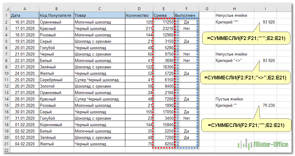
Начнем с самого простого. Предположим, у нас есть данные о продажах шоколада. Рассчитаем различные варианты продаж.
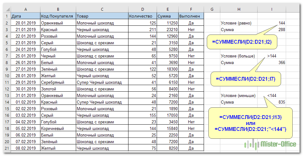
В I3 записано:
=СУММЕСЛИ(D2:D21;I2)
D2:D21 – это координаты, в которых мы ищем значение.
I2 – ссылка на критерий отбора. Иначе говоря, мы ищем ячейки со значением 144 и складываем их.
Поскольку третий параметр функции не указан, то мы сразу складываем отобранные числа. Область поиска будет одновременно являться и диапазоном суммирования.
Кроме того, в качестве задания для отбора нужных значений можно указать текстовое выражение, состоящее из знаков >, <, <>, <= или >= и числа.
Можно указать его прямо в формуле, как это сделано в I13
=СУММЕСЛИ(D2:D21;«<144»)
То есть подытоживаем все заказы, в которых количество меньше 144.
Но, согласитесь, это не слишком удобно, поскольку нужно корректировать саму формулу, да и условие еще нужно не забыть заключить в кавычки.
В дальнейшем мы будем стараться использовать только ссылку на критерий, поскольку это значительно упрощает возможные корректировки.
Критерии для текста.
Гораздо чаще встречаются ситуации, когда поиск нужно проводить в одном месте, а в другом — суммировать данные, соответствующие найденному.
Чаще всего это необходимо, если необходимо использовать отбор по определённым словам. Ведь текстовые значения складывать нельзя, а вот соответствующие им числа – можно.
Как простой прием использования формулы СУММ ЕСЛИ в Эксель таблицах, рассчитаем итог по выполненным заказам.

В I3 запишем выражение:
=СУММЕСЛИ(F2:F21;I2;E2:Е21)
F2:F21 – это область, в которой мы отбираем подходящие значения.
I2 – здесь записано, что именно отбираем.
E2:E21 – складываем числа, соответствующие найденным совпадениям.
Конечно, можно указать параметр отбора прямо в выражении:
=СУММЕСЛИ(F2:F21;”Да”;E2:Е21)
Но мы уже договорились, что так делать не совсем рационально.
Важное замечание. Не забываем, что все текстовые значения необходимо заключать в кавычки.
Подстановочные знаки для частичного совпадения.
При работе с текстовыми данными часто приходится производить поиск по какой-то части слова или фразы.
Вернемся к нашему случаю. Определим, сколько всего было заказов на черный шоколад. В результате, у нас есть 2 подходящих наименования товара. Как учесть их оба? Для этого есть понятие неточного соответствия.
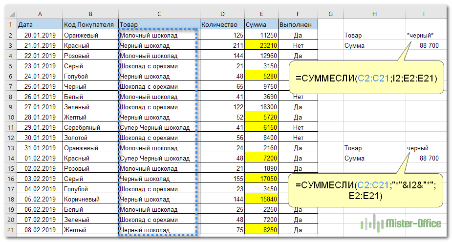
Мы можем производить поиск и подсчет значений, указывая не всё содержимое ячейки, а только её часть. Таким образом мы можем расширить границы поиска, применив знаки подстановки “?”, “*”.
Символ “?” позволяет заменить собой один любой символ.
Символ ”*” позволяет заменить собой не один, а любое количество символов (в том числе ноль).
Эти знаки можно применить в нашем случае двумя способами. Либо прямо вписать их в таблицу –
=СУММЕСЛИ(C2:C21;I2;E2:Е21) , где в E2 записано *[слово]*
либо
=СУММЕСЛИ(C2:C21;»*»&I2&»*»;E2:E21)
где * вставлены прямо в выражение и «склеены» с нужным текстом.
Давайте потренируемся:
- “*черный*” — мы ищем фразу, в которой встречается это выражение, а до него и после него – любые буквы, знаки и числа. В нашем случае этому соответствуют “Черный шоколад” и “Супер Черный шоколад”.
- “Д?” — необходимо слово из 2 букв, первая из которых “Д”, а вторая – любая. В нашем случае подойдет “Да”.
- “???” — найдем слово из любых 3 букв
=СУММЕСЛИ(F2:F21;”???”;E2:E21)
Этому требованию соответствует “Нет”.
- “???????*” — текст из любых 7 и более букв.
=СУММЕСЛИ(B2:B21;“???????*”;E8:E28)
Подойдет “Зеленый”, “Оранжевый”, “Серебряный”, “Голубой”, “Коричневый”, “Золотой”, “Розовый”.
- “З*” — мы выбираем фразу, первая буква которой “З”, а далее – любые буквы, знаки и числа. Это “Золотой” и “Зеленый”.
- “Черный*” — подходит фраза, которая начинаются именно с этого слова, а далее – любые буквы, знаки и числа. Подходит “Черный шоколад”.
Примечание. Если вам необходимо в качестве задания для поиска применять текст, который содержит в себе * и ?, то используйте знак тильда (~), поставив его перед этими символами. Тогда * и ? будут считаться обычными символами, а не шаблоном:
=СУММЕСЛИ(B2:B21;“*~?*”;E8:E28)
Важное замечание. Если в вашем тексте для поиска встречается несколько знаков * и ?, то тильду (~) нужно поставить перед каждым из них. К примеру, если мы будем искать текст, состоящий из трех звездочек, то формулу ЕСЛИ СУММ можно записать так:
=СУММЕСЛИ(B2:B21;“~*~*~*”;E8:E28)
А если текст просто содержит в себе 3 звездочки, то можно наше выражение переписать так:
=СУММЕСЛИ(B2:B21;“*~*~*~**”;E8:E28)
Точная дата либо диапазон дат.
Если нам нужно найти сумму чисел, соответствующих определённой дате, то проще всего в качестве критерия указать саму эту дату.
Примечание. При этом не забывайте, что формат указанной вами даты должен соответствовать региональным настройкам вашей таблицы!
Обратите внимание, что мы также можем здесь вписать ее прямо в формулу, а можем использовать ссылку.

Рассчитываем итог продаж за сегодняшний день – 04.02.2020г.
=СУММЕСЛИ(A2:A21;I1;E2:E21)
или же
=СУММЕСЛИ(A2:A21;СЕГОДНЯ();E2:E21)
Рассчитаем за вчерашний день.
=СУММЕСЛИ(A2:A21;СЕГОДНЯ()-1;E2:E21)
СЕГОДНЯ()-1 как раз и будет «вчера».
Складываем за даты, которые предшествовали 1 февраля.
=СУММЕСЛИ(A2:A21;»<«&»01.02.2020»;E2:E21)
После 1 февраля включительно:
=СУММЕСЛИ(A2:A21;»>=»&»01.02.2020″;E2:E21)
А если нас интересует временной интервал «от-до»?
Мы можем рассчитать итоги за определённый период времени. Для этого применим маленькую хитрость: разность функций СУММЕСЛИ. Предположим, нам нужна выручка с 1 по 4 февраля включительно. Из продаж после 1 февраля вычитаем все, что реализовано после 4 февраля.
=СУММЕСЛИ(A2:A21;»>=»&»01.02.2020″;E2:E21) — СУММЕСЛИ(A2:A21;»>=»&»04.02.2020″;E2:E21)
Сумма значений, соответствующих пустым либо непустым ячейкам
Случается, что в качестве условия суммирования нужно использовать все непустые клетки, в которых есть хотя бы одна буква, цифра или символ.
Рассмотрим ещё один вариант использования формулы СУММ ЕСЛИ в таблице Excel, где нам необходимо подсчитать заказы, в которых нет отметки о выполнении, а также сколько было вообще обработанных заказов.
Если критерий указать просто “*”, то мы учитываем для подсчета непустые ячейки, в которых имеется хотя бы одна буква или символ (кроме пустых).
=СУММЕСЛИ(F2:F21;»*»;E2:E21)
Точно такой же результат даёт использование вместо звездочки пары знаков «больше» и «меньше» — <>.
=СУММЕСЛИ(F2:F21;»<>»;E2:E21)
Теперь рассмотрим, как можно находить сумму, соответствующую пустым ячейкам.
Для того, чтобы найти пустые, в которых нет ни букв, ни цифр, в качестве критерия поставьте парные одинарные кавычки ‘’, если значение критерия указано в ячейке, а формула ссылается на неё.
Если же указать на отбор только пустых ячеек в самой формуле СУММ ЕСЛИ, то впишите двойные кавычки.
=СУММЕСЛИ(F2:F21;«»;E2:E21)
Сумма по нескольким условиям.
Функция СУММЕСЛИ может работать только с одним условием, как мы это делали ранее. Но очень часто случается, что нужно найти совокупность данных, удовлетворяющих сразу нескольким требованиям. Сделать это можно как при помощи некоторых хитростей, так и с использованием других функций. Рассмотрим все по порядку.
Вновь вернемся к нашему случаю с заказами. Рассмотрим два условия и посчитаем, сколько всего сделано заказов черного и молочного шоколада.
1. СУММЕСЛИ + СУММЕСЛИ

Все просто:
=СУММЕСЛИ($C$2:$C$21;»*»&H3&»*»;$E$2:$E$21)+СУММЕСЛИ($C$2:$C$21;»*»&H4&»*»;$E$2:$E$21)
Находим сумму заказов по каждому виду товара, а затем просто их складываем. Думаю, с этим вы уже научились работать :).
Это самое простое решение, но не самое универсальное и далеко не единственное.
2. СУММ и СУММЕСЛИ с аргументами массива.
Вышеупомянутое решение очень простое и может выполнить работу быстро, когда критериев немного. Но если вы захотите работать с несколькими, то она станет просто огромной. В этом случае лучшим подходом является использование в качестве аргумента массива критериев. Давайте рассмотрим этот подход.

Вы можете начать с перечисления всех ваших условий, разделенных запятыми, а затем заключить итоговый список, разделенный точкой с запятой, в {фигурные скобки}, который технически называется массивом.
Если вы хотите найти покупки этих двух товаров, то ваши критерии в виде массива будут выглядеть так:
СУММЕСЛИ($C$2:$C$21;{«*черный*»;»*молочный*»};$E$2:$E$21)
Поскольку здесь использован массив критериев, то результатом вычислений также будет массив, состоящий из двух значений.
А теперь воспользуемся функцией СУММ, которая умеет работать с массивами данных, складывая их содержимое.
=СУММ(СУММЕСЛИ($C$2:$C$21;{«*черный*»;»*молочный*»};$E$2:$E$21))
Важно, что результаты вычислений в первом и втором случае совпадают.
3. СУММПРОИЗВ и СУММЕСЛИ.
А если вы предпочитаете перечислять критерии в какой-то специально отведенной для этого части таблицы? Можете использовать СУММЕСЛИ в сочетании с функцией СУММПРОИЗВ, которая умножает компоненты в заданных массивах и возвращает сумму этих произведений.

Вот как это будет выглядеть:
=СУММПРОИЗВ(СУММЕСЛИ(C2:C21;H3:H4;E2:E21))
в H3 и H4 мы запишем критерии отбора.
Но, конечно, ничто не мешает вам перечислить значения в виде массива критериев:
=СУММПРОИЗВ(СУММЕСЛИ(C2:C21;{«*черный*»;»*молочный*»};E2:E21))
Результат, возвращаемый в обоих случаях, будет идентичен тому, что вы наблюдаете на скриншоте.
Важное замечание! Обратите внимание, что все перечисленные выше три способа производят расчет по логическому ИЛИ. То есть, нам нужны продажи шоколада, который будет или черным, или молочным.
Почему СУММЕСЛИ у меня не работает?
Этому может быть несколько причин. Иногда ваше выражение не возвращает того, что вы ожидаете, только потому, что тип данных в ячейке или в каком-либо аргументе не подходит для нее. Итак, вот что нужно проверить.
1. «Диапазон данных» и «диапазон суммирования» должны быть указаны ссылками, а не в виде массива.
Первый и третий атрибуты функции всегда должны быть ссылкой на область таблицы, например A1: A10. Если вы попытаетесь передать что-нибудь еще, например, массив {1,2,3}, Excel выдаст сообщение об ошибке.
Правильно: =СУММЕСЛИ(A1:A3, «цвет», C1:C3)
Неверно : =СУММЕСЛИ({1,2,3}, «цвет», C1:C3)
2. Ошибка при суммировании значений из других листов или рабочих книг.
Как и любая другая функция Excel, СУММЕСЛИ может ссылаться на другие листы и рабочие книги, если они в данный момент открыты.
Найдем сумму значений в F2: F9 на листе 1 книги 1, если соответствующие данные записаны в столбце A, и если среди них содержатся «яблоки»:
=СУММЕСЛИ([Книга1.xlsx]Лист1!$A$2:$A$9,»яблоки»,[Книга1.xlsx]Лист1!$F$2:$F$9)
Однако это перестанет работать, как только Книга1 будет закрыта. Это происходит потому, что области, на которые ссылаются формулы в закрытых книгах, преобразуются в массивы и хранятся в таком виде в текущей книге. А поскольку в аргументах 1 и 3 массивы не допускаются, то формула выдает ошибку #ЗНАЧ!.
3. Чтобы избежать проблем, убедитесь, что диапазоны данных и поиска имеют одинаковый размер.
Как отмечалось в начале этого руководства, в современных версиях Microsoft Excel они не обязательно должны иметь одинаковый размер. Но вот в Excel 2000 и более ранних версиях это может вызвать проблемы. Однако, даже в самых последних версиях Excel сложные выражения, в которых диапазон сложения имеет меньше строк и/или столбцов, чем диапазон поиска, являются капризными. Вот почему рекомендуется всегда иметь их одинакового размера и формы.
Примеры расчета суммы:

This Excel tutorial explains how to use the Excel SUMIF function with syntax and examples.
Description
The SUMIF function is a worksheet function that adds all numbers in a range of cells based on one criteria (for example, is equal to 2000).
The SUMIF function is a built-in function in Excel that is categorized as a Math/Trig Function. It can be used as a worksheet function (WS) in Excel. As a worksheet function, the SUMIF function can be entered as part of a formula in a cell of a worksheet.
To add numbers in a range based on multiple criteria, try the SUMIFS function.
![]() Subscribe
Subscribe
If you want to follow along with this tutorial, download the example spreadsheet.
Download Example
Syntax
The syntax for the SUMIF function in Microsoft Excel is:
SUMIF( range, criteria, [sum_range] )
Parameters or Arguments
- range
- The range of cells that you want to apply the criteria against.
- criteria
- The criteria used to determine which cells to add.
- sum_range
- Optional. It is the range of cells to sum together. If this parameter is omitted, it uses range as the sum_range.
Returns
The SUMIF function returns a numeric value.
Applies To
- Excel for Office 365, Excel 2019, Excel 2016, Excel 2013, Excel 2011 for Mac, Excel 2010, Excel 2007, Excel 2003, Excel XP, Excel 2000
Type of Function
- Worksheet function (WS)
Example (as Worksheet Function)
Let’s explore how to use SUMIF as a worksheet function in Microsoft Excel.
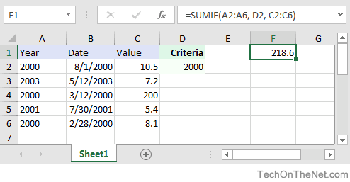
Based on the Excel spreadsheet above, the following SUMIF examples would return:
=SUMIF(A2:A6, D2, C2:C6)
Result: 218.6   'Criteria is the value in cell D2

=SUMIF(A:A, D2, C:C)
Result: 218.6   'Criteria applies to all of column A (ie: A:A)

=SUMIF(A2:A6, 2003, C2:C6)
Result: 7.2     'Criteria is the number 2003

=SUMIF(A2:A6, ">=2001", C2:C6)
Result: 12.6    'Criteria is greater than or equal to 2001

=SUMIF(C2:C6, "<100")
Result: 31.2    'Adds values in C2:C6 that are less than 100 (3rd parameter is omitted)
Now, let’s look at the example =SUMIF(A2:A6, D2, C2:C6) that returns a value of 218.6 and take a closer look why.
First Parameter
The first parameter in the SUMIF function is the range of cells that you want to apply the criteria against.
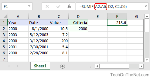
In this example, the first parameter is A2:A6. This is the range of cells that will be tested to determine if they meet the criteria.
Second Parameter
The second parameter in the SUMIF function is the criteria that will be applied against the range, A2:A6.
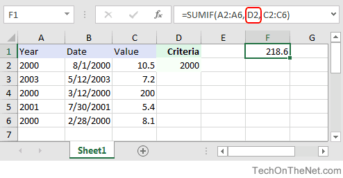
In this example, the second parameter is D2. This is a reference to the cell D2 which contains the numeric value, 2000. The SUMIF function will test each value in A2:A6 to see if it is equal to 2000.
Third Parameter
The third parameter in the SUMIF function is the range of numbers that will potentially be added together.
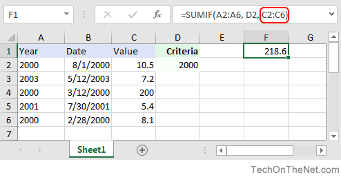
In this example, the third parameter is C2:C6. For every value in A2:A6 that matches D2, the corresponding value in C2:C6 will be summed.
Using Named Ranges
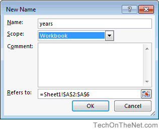
You can also use a named range in the SUMIF function. A named range is a descriptive name for a collection of cells or range in a worksheet. If you are unsure of how to setup a named range in your spreadsheet, read our tutorial on Adding a Named Range.
For example, if we created a named range called years in our spreadsheet that refers to cells A2:A6 in Sheet1 (Notice that the named range is an absolute reference that refers to =Sheet1!$A$2:$A$6 in the image below):
We could use this named range in our current example.
This would allow us to replace A2:A6 as the first parameter with the named range called years, as follows:
=SUMIF(A2:A6, D2, C2:C6)    'First parameter uses a standard range
Result: 218.6

=SUMIF(years, D2, C2:C6)    'First parameter uses a named range called years
Result: 218.6
Frequently Asked Questions
Question: I have a question about how to write the following formula in Excel.
I have a few cells, but I only need the sum of all the negative cells. So if I have 8 values, A1 to A8 and only A1, A4 and A6 are negative then I want B1 to be sum(A1,A4,A6).
Answer: You can use the SUMIF function to sum only the negative values as you described above. For example:
=SUMIF(A1:A8,"<0")
This formula would sum only the values in cells A1:A8 where the value is negative (ie: <0).
Question:In Microsoft Excel I’m trying to achieve the following with IF function:
If a value in any cell in column F is «food» then add the value of its corresponding cell in column G (eg a corresponding cell for F3 is G3). The IF function is performed in another cell altogether. I can do it for a single pair of cells but I don’t know how to do it for an entire column. Could you help?
At the moment, I’ve got this:
=IF(F3="food"; G3; 0)
Answer:This formula can be created using the SUMIF formula instead of using the IF function:
=SUMIF(F1:F10,"=food",G1:G10)
This will evaluate the first 10 rows of data in your spreadsheet. You may need to adjust the ranges accordingly.
I notice that you separate your parameters with semi-colons, so you might need to replace the commas in the formula above with semi-colons.
Probably everyone can summarize data in Excel program. But with the improved version of the SUM function, which is called SUMIF, the capabilities of this operation are significantly expanded.
By the name of the function, you can understand that it does not only calculate the sum, but also complies with some logical conditions.
SUMIF and its syntax
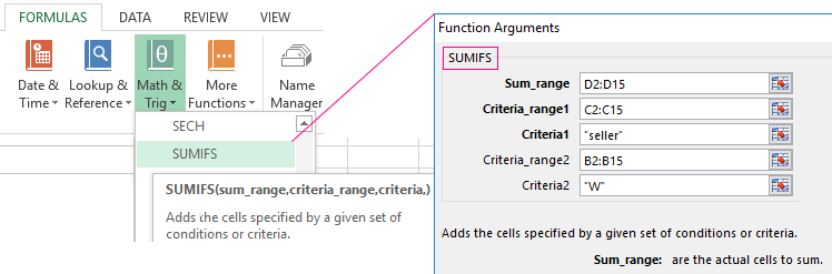
The SUMIF function allows you to sum cells that meet a certain criterion (a given condition). The arguments of the function are as follows:
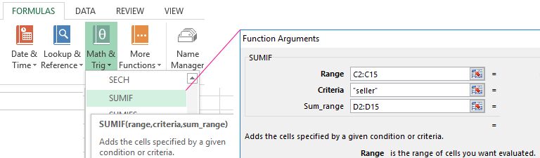
- Range — cells, which should be evaluated on the basis of the criterion (the specified condition).
- Criteria, determining which cells from the range will be selected (written in quotation marks).
- Sum range — the actual cells that are needed to be summed if they meet the criterion.
Consequently the function has only 3 arguments. However, sometimes the third one can be excluded, and then the command will work only by the range and criteria.
How does the SUMIF function work in Excel?
Let’s consider the simplest example, which will clearly demonstrate how to use the SUMIF function and how convenient it can be for solving certain tasks.
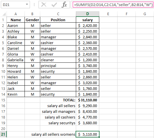
We have a table in which the names of employees, their gender and salary, calculated for January are indicated. If we just need to calculate the total amount of money that is required to pay out to employees, we use the SUM function, specifying all salaries by the range.
But what do we have to do if we need to quickly calculate only sellers’ salaries? In this case, the use of the SUMIF function will help.
Enter the arguments.
- The range in this case will be a list of all staff posts, because we will need to determine the whole amount of salaries. Therefore, enter E2:E14.
- The criterion of choice in our case is the seller. Enclose the word in quotation marks and put it as the second argument.
- The range of summation is salaries, because we need to know the amount of salaries of all sellers. Therefore, enter F2:F14.
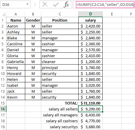
We have obtained 9290$. It means that the function automatically elaborated the list of all posts, chose only sellers from them and summed up their salaries.
Similarly, you can calculate the salaries of all managers, vendors, cashiers and security guards. When the table is small, it seems that everything can be counted manually, but when working with lists having several hundreds of positions, it makes sense to use SUMIF function.
SUMIF function in Excel with multiple criteria SUMIFS
If the letter S is added to the end of the standard SUMIF command, then it implies the function with several criteria (SUMIFS function). It is used in the case when you need to specify more than one criterion.
Syntax of using the function by several criteria
There can be as many arguments for SUMIFS as you like, but no less than 5.
- Sum range. If in SUMIF it was at the end, then here it is in the first place. It also indicates the cells that need to be summed.
- Criteria range 1 — cells that need to be evaluated on the basis of the first criterion.
- Criteria 1 — defines the cells that the function will select from the first range of the condition.
- Criteria range 2 — cells, which should be evaluated on the basis of the second criterion.
- Criteria 2 — defines the cells that the function will select from the second condition range.
And so on. Depending on the number of criteria, the number of arguments can increase in an arithmetic progression in step 2. That is, 5, 7, 9 …
Example of use
Suppose we need to calculate the amount of salaries of all female sellers for January. We have two conditions. The employee must be:
- a seller;
- a woman.
So, we will use the SUMIFS command.
Enter the arguments.
- Sum range — cells with a salary;
- Criteria range 1 — cells indicating the post of the employee;
- Criteria 1 — the seller;
- Criteria range 2 — cells with gender of the employee;
- Criteria 2 — female (f).
The result: all female sellers in January received in summation 5110$.
SUMIF in Excel with dynamic criterion
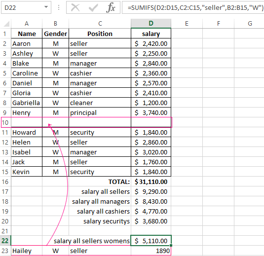
The SUMIF and SUMIFS functions are useful because they automatically fit themselves to the changing criteria. That is, we can change the data in cells, and the sums will change with them. For example, when calculating salaries, it turned out that we forgot to take into account one employee who works as a seller. We can add one more line by right-clicking and selecting the ВСТАВИТЬ command.
We have an additional row. We can see that the range of conditions and summations has automatically expanded to 15 rows.
Copy the employee’s data and paste it into the general list. The sums in the resulting cells have changed. The functions have reacted to the appearance of another female seller in the range.
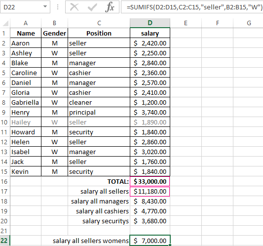
Similarly, you can not only add, but also delete any rows (for example, when the employee is discharged), change the values, etc.
The SUMIF Excel function calculates the sum of a range of cells based on given criteria. The criteria can include dates, numbers, and text. For example, the formula “=SUMIF(B1:B5, “<=12”)” adds the values in the cell range B1:B5, which are less than or equal to 12.
SUMIF function is categorized under the Excel Math and Trigonometry functions. Moreover, this function works similar to the SUMIFS functionSUMIFS is an enhanced version of the SUMIF formula in Excel that enables you to sum any range of data by matching several criteria. read more. The SUMIF function uses a single criterion, whereas the SUMIFS function uses multiple criteria.
Table of contents
- SUMIF in Excel
- SUMIF Formula in Excel
- How to Use the SUMIF Excel Function?
- Example #1
- Example #2
- Example #3
- Example #4
- The “Criteria” Argument of the SUMIF Function
- Frequently Asked Questions (FAQs)
- SUMIF Excel Function Video
- Recommended Articles
SUMIF Formula in Excel
The SUMIF formula is stated as follows:

The formula accepts the following arguments:
- Range: It refers to the range of cells on which the criteria is applied.
- Criteria: It refers to the conditions that are applied to the range of cells. It determines the cells to be added from the given “sum_range.”
- Sum_range: It indicates the range of cells to be added together.
“Range” and “criteria” are the required parameters, whereas “sum_range” is an optional parameter.
Note: If “sum_range” is not specified, the SUMIF function refers to the parameter “range” as the range of cells to be added.
How to Use the SUMIF Excel Function?
Let us understand the SUMIF excel function with the help of the following examples. Each example covers a different case, implemented using the SUMIF function.
You can download this SUMIF Function in Excel Template here – SUMIF Function in Excel Template
Example #1
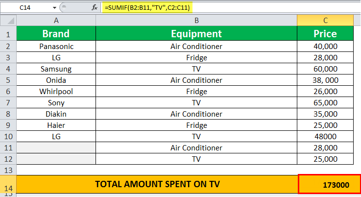
Total Amount Spent on Branded Televisions (TVs)
The following table shows a list of branded equipment and their prices. For some equipment, the brands are not specified. We have to calculate the total amount spent on purchasing branded TVs using the SUMIF function.
In the succeeding table, the cells that satisfy the given criteria are C4, C7, and C10, which shows the prices of the branded TVs. Hence, the sum of the values of cells C4, C7, and C10 is 1,73,000, shown in cell C14. This is the total amount spent on purchasing branded TVs.
The following SUMIF formula is applied to the range C2:C11:
“=SUMIF(B2:B11,“TV”,C2:C11)”
Where,
- B2:B11 refers to the range of cells on which the specific criterion is to be applied.
- “TV” refers to the condition applied to the range B2:B11.
- C2:C11 refers to the range of values to be added.
Example #2
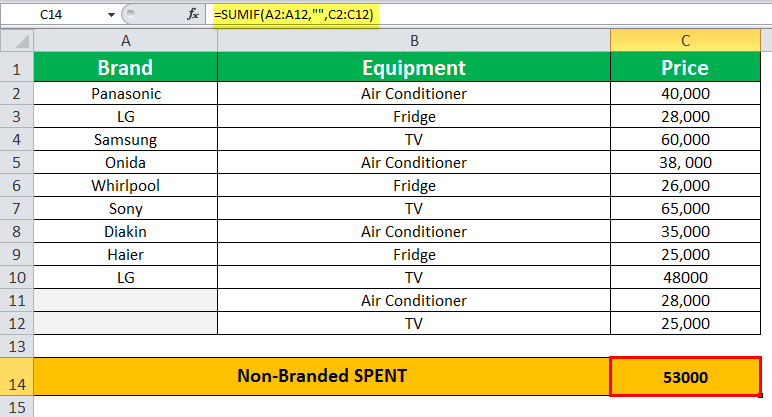
Sum of the Amount Spent on Non-Branded Items
Working on the data of example #1, we want to calculate the total amount spent on purchasing non-branded items using the SUMIF function.
In the following table, the cells C11 and C12 satisfy the given criteria where no brand name is entered in the cells. Hence, the sum of the values of cells C11and C12 is 53,000, as shown in cell C14. This indicates the total amount spent on purchasing non-branded items.
The following SUMIF formula is applied to the range C2:C12:
“=SUMIF(A2:A12,“”,C2:C12)”
Where,
- A2:A12 refers to the range of cells on which the specific criterion is to be applied.
- “” refers to the condition which checks for blank cells in the range B2:B12.
- C2:C12 is the range of values to be summed up.
Example #3
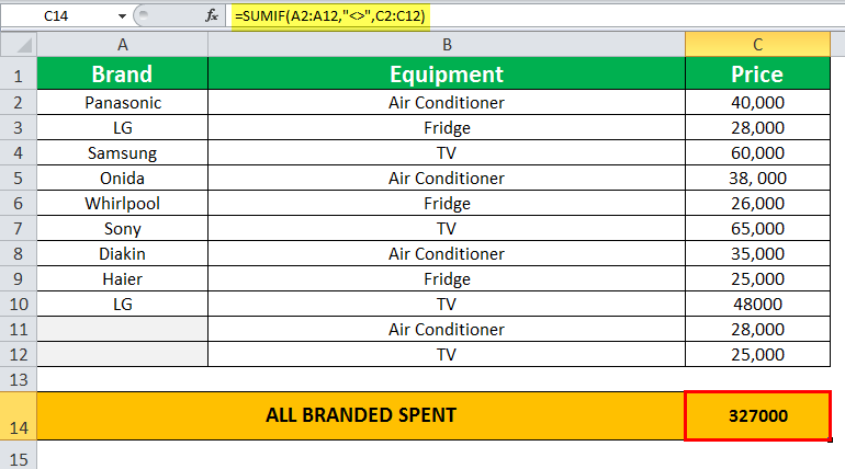
Sum of the Amount Spent on Branded Items
Working on the data of example #1, we want to calculate the total amount spent on branded items using the SUMIF function.
In the following table, the cells B11, B12 satisfy the given criteria with no brand names. Hence, the sum of the values of C1 to C10 is 53,000, displayed in cell C14. This is the total amount spent on purchasing branded items. The cells C11 and C12 are skipped because they are blank cells.
The following SUMIF formula is applied to the range C2:C12:
“=SUMIF(A2:A12,“<>”,C2:C12)”
Where,
- A2:A12 refers to the range on which the criteria are to be applied.
- “<>” is the condition which checks for non-blank cells in the range B2:B12.
- C2:C12 is the range of values to be added.
Example #4
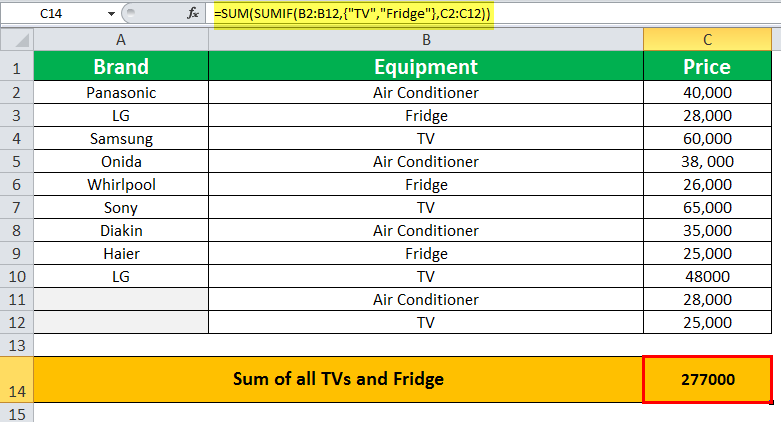
Sum of the Two Different Items
Working on the data of example #1, we want to calculate the sum of two different items using the SUMIF formula.
The following table shows the total amount calculated by adding the sum of the prices of two items – TV and fridge in the cell C14, using the SUMIF formula. The SUM of the prices of the fridges and TVs are 79,000 and 1,98,000, respectively. Hence, the total SUM of the prices of two items is 2,77,000.
The SUMIF formula is applied to the range C2:C12 and is stated as follows:
“=SUM(SUMIF(B2:B12,{“TV”,“Fridge”},C2:C12))”
Where,
- B2: B12 refers to the range on which the criteria are to be applied.
- “TV,” “fridge” refers to the two individual conditions to be checked in range B2: B12. The curly braces {} of the criterion represent the collection of constants.
- C2: C12 refers to the range of values to be added.
In the formula, the SUMIF function is enclosed within the SUM function. The SUMIF formula executes two different conditions, “TV” and “fridge.” Finally, the SUM functionThe SUM function in excel adds the numerical values in a range of cells. Being categorized under the Math and Trigonometry function, it is entered by typing “=SUM” followed by the values to be summed. The values supplied to the function can be numbers, cell references or ranges.read more sums the results of the SUMIF functions to return the output.
The “Criteria” Argument of the SUMIF Function
The guidelines of the argument of the SUMIF formula are stated as follows:
- The numeric criteria are not enclosed in double quotes.
- The text criteria for SUMIFSUMIF function is a conditional IF function to sum the cells based on specific criteria. For example, to add a group of cells, if the cell adjacent to them has a specified text in them, then function is used as follows =SUMIF(Text Range,” Text”, cells range for sum).read more, including the mathematical symbols, are enclosed within double quotes.
- The wildcard characters – question mark (?) and asterisk (*) used in the criteria match a single character and a series of characters, respectively.
- The tilde operator (~) followed by the wildcard characters refer to the actual characters. For example, the “~?” indicates criteria as a question mark literally.
- The SUMIF formula returns “#VALUE! error” when the criterion is a text string that is greater than 255 characters.
Frequently Asked Questions (FAQs)
1. What is the SUMIF function in Excel?
The SUMIF function returns the sum of cells that satisfy the given criteria. This worksheet (WS) function is categorized as a Math and Trigonometry function. Furthermore, for partial matching, it uses logical operators and wildcards.
The SUMIF formula is stated as follows:
“=SUMIF(range, criteria, [sum_range])”
Where,
• Range refers to the range of cells against which we need to apply the criteria.
• Criteria are the conditions that are applied to the range of cells.
• Sum_range is an array of numeric values. The values are added if the specific criterion matches the range.
The “range” and “criteria” are the required arguments, and “sum_range” is an optional argument.
Note: If the argument “sum_range” is omitted, the values in the “range” will be added.
2. How to use the SUMIF Excel function for multiple criteria?
The formula for the SUMIF with multiple criteria is stated as follows:
“=SUMIF(sum_range, range 1, criteria1)+SUMIF(sum_range, range 2, criteria2)”
Where,
• Sum_range refers to the range of cells to be added.
• Range1, range 2 are the range of cells on which the criteria are to be applied.
• Criteria1, criteria 2 are the conditions applied to the respective range of cells. Alternatively, we can use the SUMIFS function to sum cells satisfying the multiple criteria.
3. Can we use the SUMIF function with text criteria?
The SUMIF excel function can be used to add cells containing text strings that meet specific criteria. In the formula, the text criteria are enclosed in double quotes.
For example, consider the below SUMIF formula:
“=SUMIF(A1:A4,“Purple”,B1:B4)”
The formula adds the values in range B1:B4 if the range A1:A4 contains the text “Purple”.
SUMIF Excel Function Video
Recommended Articles
This has been a guide to SUMIF Excel Function. Here we discuss how to use SUMIF Formula along with excel examples and downloadable templates. You may also look at these useful functions in Excel –
- Excel SUM ShortcutThe Excel SUM Shortcut is a function that is used to add up multiple values by simultaneously pressing the “Alt” and “=” buttons in the desired cell. However, the data must be present in a continuous range for this function to function.read more
- SUMIF With VLOOKUPSUMIF is used to sum cells based on some condition, which takes arguments of range, criteria, or condition, and cells to sum. When there is a large amount of data available in multiple columns, we can use VLOOKUP as the criteria.read more
- Excel SUMIF Between Two DatesWhen we wish to work with data that has serial numbers with different dates and the condition to sum the values is based between two dates, we use Sumif between two dates. read more
- SUM in ExcelThe SUM function in excel adds the numerical values in a range of cells. Being categorized under the Math and Trigonometry function, it is entered by typing “=SUM” followed by the values to be summed. The values supplied to the function can be numbers, cell references or ranges.read more