
How to correct a #NUM! error
Excel for Microsoft 365 Excel for Microsoft 365 for Mac Excel for the web Excel 2021 Excel 2021 for Mac Excel 2019 Excel 2019 for Mac Excel 2016 Excel 2016 for Mac Excel 2013 Excel for iPad Excel Web App Excel for iPhone Excel for Android tablets Excel 2010 Excel 2007 Excel for Mac 2011 Excel for Android phones Excel for Windows Phone 10 Excel Mobile Excel Starter 2010 More…Less
Excel shows this error when a formula or function contains numeric values that aren’t valid.
This often happens when you’ve entered a numeric value using a data type or a number format that’s not supported in the argument section of the formula. For example, you can’t enter a value like $1,000 in currency format, because dollar signs are used as absolute reference indicators and commas as argument separators in formulas. To avoid the #NUM! error, enter values as unformatted numbers, like 1000, instead.
Excel might also show the #NUM! error when:
-
A formula uses a function that iterates, such as IRR or RATE, and it can’t find a result.
To fix this, change the number of times Excel iterates formulas:
-
Select File > Options. If you are using Excel 2007, select Microsoft Office Button
 > Excel Options.
 -
On the Formulas tab, under Calculation options, check the Enable iterative calculation box.
-
In the Maximum Iterations box, type the number of times you want Excel to recalculate. The higher the number of iterations, the more time Excel needs to calculate a worksheet.
-
In the Maximum Change box, type the amount of change you’ll accept between calculation results. The smaller the number, the more accurate the result and the more time Excel needs to calculate a worksheet.
-
-
A formula results in a number that’s too large or too small to be shown in Excel.
To fix this, change the formula so that its result is between -1*10307 and 1*10307.
Tip: If error checking is turned on in Excel, you can click
next to cell that shows the error. Click Show Calculation Steps if it’s available, and pick the resolution that works for your data.
 > Excel Options.
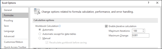
 next to cell that shows the error. Click Show Calculation Steps if it’s available, and pick the resolution that works for your data.
Need more help?
You can always ask an expert in the Excel Tech Community or get support in the Answers community.
See Also
Overview of formulas in Excel
How to avoid broken formulas
Detect errors in formulas
Excel functions (alphabetical)
Excel functions (by category)
Need more help?
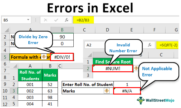
List of Various Excel Errors
MS Excel is popular for only its most useful automatic calculation feature, which we achieve by applying various functions and formulas. But while using formulas in Excel cell, we get multiple types of errors.
Table of contents
- List of Various Excel Errors
- Types of Errors in Excel with Examples
- 1 – #DIV/0 Error
- How to Resolve this Error?
- Example – IF Function to Avoid #DIV/0 Error
- 2 – #N/A Error
- Solution 1: To enter the Roll number as text
- Solution 2: Use the TEXT Function
- 3 – #NAME? Error
- 4 – #NULL! Error
- 5 – #NUM! Error
- Example 1
- Example 2
- 6 – #REF! Error
- 7 – #VALUE! Error
- 8 – ###### Error
- Example
- 9 – Circular Reference Error
- 1 – #DIV/0 Error
- Function to Deal with Excel Errors
- 1 – ISERROR Function
- 2 – AGGREGATE Function
- Example
- Things to Remember
- Recommended Articles
- Types of Errors in Excel with Examples
The error can be:
- #DIV/0
- #N/A
- #NAME?
- #NULL!
- #NUM!
- #REF!
- #VALUE!
- #####
- Circular Reference
We have various functions to deal with these errors, which are –
- IFERROR Function
- ISERROR FunctionISERROR is a logical function that determines whether or not the cells being referred to have an error. If an error is found, it returns TRUE; if no errors are found, it returns FALSE.read more
- AGGREGATE Function
Types of Errors in Excel with Examples
You can download this Errors Excel Template here – Errors Excel Template
1 – #DIV/0 Error
#DIV/0! Error is received when we work with a spreadsheet formula, which divides two values in a formula and the divisor (the number being divided by) is zero. It stands for divide by zero error.
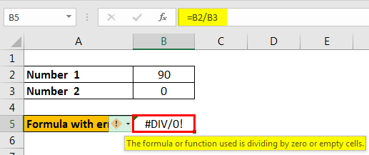
Here, in the above image, we see that number 90 is divided by 0. That is why we get the #DIV/0! Error.
How to Resolve this Error?
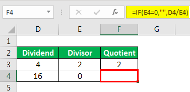
The first and foremost solution is to divide only with cells with a value not equal to zero. But there are situations when we also have empty cells in a spreadsheet. In that case, we can use the IF function as below.
Example – IF Function to Avoid #DIV/0 Error
Follow the steps below to use the IF function to avoid the #DIV/0! Error.
- Suppose we are getting a #DIV/0! Error as follows:

- To avoid this error, we can use the IF function as follows:


2 – #N/A Error
This error means “no value available” or “not available.” It indicates that the formula cannot find the value that we suppose it may return.
For example, using Excel’s VLOOKUP, HLOOKUP, MATCHThe MATCH function looks for a specific value and returns its relative position in a given range of cells. The output is the first position found for the given value. Being a lookup and reference function, it works for both an exact and approximate match. For example, if the range A11:A15 consists of the numbers 2, 9, 8, 14, 32, the formula “MATCH(8,A11:A15,0)” returns 3. This is because the number 8 is at the third position.
read more, and LOOKUP functions, we may get this error if we do not find referenced value in the source data as an argument.
- When the source data and the lookup value are not of the same data type:
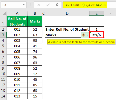
In the above example, we have entered “Roll No. of Students” as a number, but the roll numbers of students are stored as text in the source data. That is why the #N/A error appears.
To resolve this error, we can either enter the roll number as text-only or use the TEXT formula in excelTEXT function in excel is a string function used to change a given input to the text provided in a specified number format. It is used when we large data sets from multiple users and the formats are different.read more in the VLOOKUP Function.
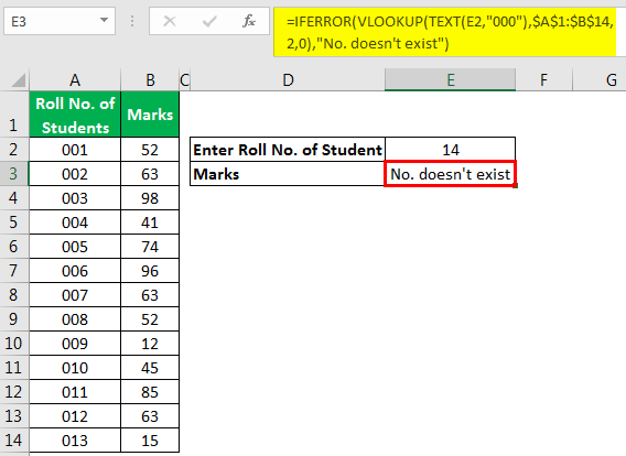
Solution 1: To enter the Roll number as text

Solution 2: Use the TEXT Function
We can use the TEXT function in the VLOOKUP function for the lookup_value argument to convert entered numbers to TEXT.

We could also use the IFERROR function in excel to display the message if VLOOKUP cannot find the referenced value in the source data.
3 – #NAME? Error
This error is displayed when we usually misspell the function name.
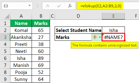
We can see in the above image that VLOOKUP is not spelled correctly; that is why #NAME? Error is being displayed.
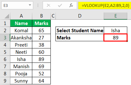
To resolve the error, we need to correct the spelling.
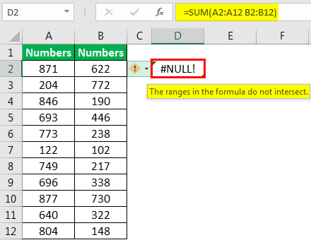
4 – #NULL! Error
This error is usually displayed when cell referencesCell reference in excel is referring the other cells to a cell to use its values or properties. For instance, if we have data in cell A2 and want to use that in cell A1, use =A2 in cell A1, and this will copy the A2 value in A1.read more are not specified correctly.
We get this error when we do not use the space character appropriately. The space character is called the “intersect operator,” which specifies the range that intersects each other at any cell.
In the below image, we have used the space character, but the ranges A2:A12 and B2:B12 are not intersecting; that is why this error is displayed.
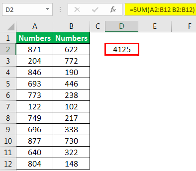
In the below image, we can see that the sum of range B2:B12 is being displayed in cell D2 as while specifying a range for SUM function, we have picked up two references (with space character), which overlap each other for range B2:B12. That is why the sum of the B2:B12 range is displayed.
#NULL! an error can also be displayed when we use intersect operator (space character) instead of:
- Mathematical Operator (Plus Sign) to sum.
- Range Operator (Colon Sign) to specify the start and end cell for a range.
- Union Operator (Comma Sign) to separate individual cell references.
5 – #NUM! Error
This error is usually displayed when a number for any function argument is found invalid.
Example 1
To find out the square root in excelThe Square Root function is an arithmetic function built into Excel that is used to determine the square root of a given number. To use this function, type the term =SQRT and hit the tab key, which will bring up the SQRT function. Moreover, this function accepts a single argument.read more of a negative number is not possible as the square of a number always has to be positive.

To solve the error, we need to make the number positive.

Example 2
MS Excel has a range of numbers that we can use. The number smaller than the shortest number or number greater than the longest number due to the function can return an error.

Here, we can see that we have written the formula as 2^8000, which yields results greater than the longest number; that is why #NUM! Error is being displayed.
6 – #REF! Error
This error stands for reference error. This error usually comes when
- We accidentally deleted the cell which we referenced in the formula.
- We cut and paste the referenced cell in different locations.

As we deleted cell B7, then cell C7 shifted left to take the place of B7, and we got a reference error in the formula as we deleted one of the referenced cells of the formula.
7 – #VALUE! Error
This error comes when we use the wrong data type for a function or formula. For example, we can add only numbers. But if we use any other data type like text, this error will be displayed.

8 – ###### Error
This error is displayed when the column width in excelA user can set the width of a column in an excel worksheet between 0 and 255, where one character width equals one unit. The column width for a new excel sheet is 8.43 characters, which is equal to 64 pixels.read more is not enough to show the stored value in the cell.
Example
In the below image, dates and times are written in the cells. But, as column width is not enough, ##### is being displayed.

To resolve the error, we need to increase the column width as per requirement using the “Column Width” command available in the “Format” menu in the “Cell Size” group under the “Home” tab, or we can double click on the right border of the column.

9 – Circular Reference Error
This type of error comes when we reference the same cell in which we are writing the function or formula.

The above image shows that we have a sum of 0 as we have referenced B4 in the B4 cell itself for calculation.
Whenever we create this type of circular reference in excelA circular reference in Excel refers to the same cell we are working on. A circular reference is a type of pop-up or warning displayed by Excel that we are using a circular reference in our formula and the calculation might be incorrect.
read more, Excel alerts us about the same too.

To resolve the error, we need to remove the reference for the B4 cell.

Function to Deal with Excel Errors
1 – ISERROR Function
This function is used to check whether there would be an error after applying the function or not.

2 – AGGREGATE Function
This function ignores error values. Therefore, when we know that there can be an error in the source data, we need to use this function instead of the SUM, COUNT function, etc.
Example
We can see that the AGGREGATE functionAGGREGATE Function in excel returns the aggregate of a given data table or data lists.read more avoids error values.

Things to Remember
- To resolve any error in the formula, we can take online help also. First, we need to click on the “Insert Function” button under the “Formulas” tab and choose “Help on this function.”

- To avoid the #NAME? Error, we can choose the desired function from the drop-down list opened when we start typing any function in the cell, followed by the “=” sign. Next, we need to press the “Tab” button on the keyboard to select a function.
Recommended Articles
This article is a guide to Errors in Excel. Here, we discuss the top types of errors in Excel and functions to deal with them with the help of examples. You can learn more about Excel from the following articles: –
- VLOOKUP Errors in Excel
- Calculate Standard Error
- Shortcut to Edit Excel Cells
- Payslip Template in Excel
The #NUM! error is a frequent visitor on your worksheet. This can make you want to pull your hair out if you’ve used the output cell as a reference in another formula.
Looking for a fix? ExcelTrick has it for you.

What is a #NUM! Error in Excel?
#NUM! error occurs when you’ve entered a formula in your worksheet, but it can’t perform the calculation. For instance, say you’re trying to find square roots for a list of numbers. But there’s a negative value in the list. The formula will return a #NUM error for this value since it’s impossible to find the square root of a negative number.
But that’s not the only reason that can invite a #NUM! error into your worksheet. There are four possibilities that could be the reason for your perils. Fixing the error typically requires adjusting the values (no, it’s not mechanical, but an arithmetic error), and you’ll be set in no time.
Why Does it Appear?
So, why do #NUM! errors occur? Yes, as mentioned, there are four reasons. Let’s talk about them in a little more detail.
We already talked about the first reason in the previous section. If you’re trying to perform an impossible calculation, for instance, finding the square root of a negative number, you’ll get a #NUM! error.
The second reason could be that the output is too large or too small. The smallest and largest numbers that Excel can handle are -1*10^308 and 1*10^308, respectively. Excel displays any output outside this range as a #NUM! error.
The third reason could be that you’ve used an iterative formula that’s not finding a result. For instance, if you’re doing some capital budgeting and you’ve used the IRR formula in the process, and you see a #NUM! error, check the IRR formula. The IRR formula tries to calculate an answer that’s accurate down to 0.00001%. It tries to run about 20 iterations to find the answer. If it doesn’t, it returns the #NUM! error.
The fourth reason could be that you’ve entered an argument incorrectly in your function. For instance, think about the DATEDIF function. Things are all smooth sailing with this delightfully simple function, unless you mistakenly enter a start date that falls after the end date.
Sounds good? Perfect, let’s now try to look at how each of these reasons could play out on your worksheet and how to fix them with examples.
Examples
Following are some examples of when you’d see a #NUM! error.
1. Fixing #NUM! error when the calculation is impossible
When you’ve inadvertently asked Excel to perform an impossible calculation, you’ll see a #NUM! error. But the fix is, well, to make the calculation possible.
Let’s use the square root problem we discussed earlier. Say you’ve got some numbers in a list that you want a square root of, and you’ve applied the following formula to the numbers.
=SQRT(A2)
A negative number has sneaked into your list and caused a #NUM! error on your other spotless spreadsheet.

Once you’ve calmed yourself down from the panic of seeing the #NUM! error, think rationally. Since it’s impossible to find the square root of a negative number, you need to make it positive. The way to make it positive? The ABS function.
Here’s the formula you should use to fix the #NUM! error.
=SQRT(ABS(A2))

The ABS function converts the negative value into a positive one. When you enter a positive value into the SQRT function, everything should work fine. Easy-peasy, eh?
2. Fixing #NUM! error when the number is too large or small
The thing is… you can’t really fix this. If your output is too large or small for Excel, you’ll need to change your input to bring the output value within the acceptable range. For instance, say you’ve performed the following arithmetic operation in your Excel sheet:
=100^500

Now, there’s no chance that Excel will be able to display this value, and will therefore return a #NUM! error. There’s no way to display the result, so you’ll need to change the output.
3. Fixing #NUM! error resulting from an iteration formula
Functions like IRR can sometimes also lead to a #NUM error. Such errors are mainly because of two reasons:
- The specified Cash flow does not contain at least one negative and one positive value.
- Formula can’t find a result.
Let’s take the first case first.
In this example, we have listed down our cash flows within the range B2:B13. Now we will try to calculate the IRR using the formula below:
=IRR(B2:B13)

As we can see in the image above, excel returns a #NUM! error. The reason is pretty simple – the IRR function requires at least one negative value in the range as the initial cost of business.
So, in order to fix such an error, we can simply add our initial cost of business as a negative value to the cashflow range and the IRR function will display a valid result.

Another case, when the IRR function returns a #NUM error is when the function iterates and can’t find a result after several tries. We know that formulas like IRR and XIRR run several iterations to find an accurate answer.
However, Excel caps the number of iterations that these formulas go through so they’re not stuck in an infinite loop. When the formula maxes out the iterations without finding an answer, it returns a #NUM! error.
To overcome this, you have the option to increase the maximum number of iterations that Excel allows to get the result.
To increase the number of allowed iterations:
- Navigate to File > Options > Formulas to arrive at the window below
- Under the Calculation options group, check the Enable iterative calculation checkbox.

- In the Maximum Iterations textbox, enter the number of times you want Excel to perform iterations. Please note that – The higher the number of iterations, the more time and resources Excel might need to consume to display the result.
4. Fixing #NUM! error when you’ve entered an incorrect function argument
You can guess the fix before even looking through the example, can’t you? All you need to do is just enter the arguments correctly. Let’s look at how this will pan out practically.
Say you’ve got a few dates listed in two columns, and you’ve decided to find the differences between those dates. You remember reading our DATEDIF function tutorial, but you make a tiny mistake.
Understandable, right? If you read the DATEDIF tutorial carefully, you’ll see that Excel doesn’t show you the arguments you need to input as you type the formula, so this could be an easy mistake.
You use the start date as the end date and vice versa while applying the formula. So, you’ve incorrectly used the following formula.
=DATEDIF(B2,A2,"d")

The fix is simply to enter the arguments correctly into the formula, and that should eliminate the #NUM! error from your worksheet.
=DATEDIF(A2,B2,"d")

That’s all the ways you can deal with the #NUM! error whenever you find it on your worksheets. Child’s walk, right? While you champion eliminating #NUM! errors, we’ve got some more tutorials lined up for you. When you’re done, you know where to find us.
Explanation
The #NUM! error occurs in Excel formulas when a calculation can’t be performed. For example, if you try to calculate the square root of a negative number, you’ll see the #NUM! error. The examples below show formulas that return the #NUM error. In general, the fixing the #NUM! error is a matter of adjusting inputs as required to make a calculation possible again.
Example #1 — Number too big or small
Excel has limits on the smallest and largest numbers you can use. If you try to work with numbers outside this range, you will receive the #NUM error. For example, raising 5 to the power of 500 is outside the allowed range:
=5^500 // returns #NUM!
Example #2 — Impossible calculation
The #NUM! error also can appear when a calculation can’t be performed. For example, the screen below shows how to use the SQRT function to calculate the square root of a number. The formula in C3, copied down, is:
=SQRT(B3)

In cell C5, the formula returns #NUM, since the calculation can’t be performed. If you need to get the square root of a negative value (treating the value as positive) you can wrap the number in the ABS function like this:
=SQRT(ABS(B3))

You could also use the IFERROR function to trap the error and return and empty result («») or a custom message.
Example #3 — incorrect function argument
Sometimes you’ll see the #NUM! error if you supply an invalid input to a function argument. For example, the DATEDIF function returns the difference between two dates in various units. It takes three arguments like this:
=DATEDIF (start_date, end_date, unit)
As long as inputs are valid, DATEDIF returns the time between dates in the unit specified. However, if start date is greater than end date, DATEDIF returns the #NUM error. In the scree below, you can see that the formula works fine until row 5, where the start date is greater than the end date. In D5, the formula returns #NUM.

Notice this is a bit different from the #VALUE! error, which typically occurs when an input value is not the right type. To fix the error shown above, just reverse the dates on row 5.
Example #4 — iteration formula can’t find result
Some Excel functions like IRR, RATE, and XIRR, rely on iteration to find a result. For performance reasons, Excel limits the number of iterations allowed. If no result is found before this limit is reached, the formula returns #NUM error. Iteration behavior can be adjusted at Options > Formulas > Calculation options.
Full List of ALL Excel Errors and How to Fix Them (2023)
Hashtags are a trend – yes, but only until they are on Instagram or maybe Twitter. As soon as you see your Excel sheet throwing hashtags your way, you know there’s something wrong 🛑
Excel errors come with a hashtag before them #️⃣
Like the #DIV/0 error, #NAME? Error and so on. And there’s always some specific reason why you’d see these errors in Excel.
Learn about that reason and remove it to fix the errors in your Excel sheet through the guide below. We have them all (the Excel errors) sorted for you here.
So glide in and download our free sample workbook on your way to tag along with the guide 📩
#DIV/0 error
The #DIV/0 error tells that you are dividing a number by zero. And let me take you back to Grade 6, where we learned that a number divided by zero is undefined 👩🏫
Practically, no number is divisible by zero. And that is why if you try dividing a number by zero in Excel, you end up with a #DIV/0 error.
For example, check this out:

Similarly, if you divide a number by a blank cell, here’s what you get.

Also, if you have a #DIV/0 error in a cell and you refer to it in any other formula, you’d still get the #DIV/0 error.
For example, here we’ve referred to Cell A2 (that contains the #DIV/0 error) in our formula =A1+A2+A3, and this is what we get 🤦♀️

The answer is again a #DIV/0 error.
Some quick ways how you can prevent the #DIV/0 error in Excel include ensuring the following:
- Your formulas do not refer to any cells containing the #DIV/0 error
- You don’t perform the division operation using any empty cells.
- The cells in your dataset do not contain zeros
In addition to these, you can also use the IFERROR function to replace the #DIV/0 error in your worksheet with any other value as desired 👌
How? Learn more details about it by reading our tutorial on the #DIV/0 error here!
#N/A error
In simple words, the #N/A error means that the underlying formula failed to find what it had been told to find.
For example, if you write the VLOOKUP function to find the sales of “P” from the data in the image below:

You’ll get the #N/A error because there is no “P” in the data above. And the VLOOKUP function is set to find the data under the exact match mode.
It fails to find the given lookup value – and we end up with a #N/A error ❌
The function might not be able to find the given value for several reasons. Maybe because it’s not in the right format, or maybe because the spelling of the look-up value doesn’t match.
You’d most likely see the #N/A error in Excel when you’re using the lookup functions i.e. VLOOKUP, HLOOKUP, MATCH, etc.
You can prevent (or fix) the #N/A error by trying the following:
- The lookup value is correctly spelled. No special characters or extra spaces to it.
- The lookup table contains the lookup values.
- The match mode (exact or approximate) is in line with the look-up value.
#NAME? error
As the name suggests, the #NAME error occurs when you have misspelled a name. It could be the name of a function, the name of a named range, or even an incorrect argument.
For example, check out here 👀

If you misspell the SUM function as the SIM function, you get the #NAME error.
Similarly, if you have saved a range by a name in Excel, misspelling it will cause the #NAME error as below.
Here the name of the range was “Numbers” and we misspelled it as “Number” 🔢

When the range is rightly spelled as “Numbers”, the results change as follows:

To avoid this problem, type in the first letter of the formula and press the “Tab” key.
Excel will enter the name of the function for you so there is no more chance of spelling mistakes.
And yeah! You’d also get the #NAME error if you wrongly write the reference for a range. Like we have forgotten the colon between A2 and A4 (A2A4 instead of A2:A4) here. So we get the #NAME? error 📍

#REF! error
The #REF error is Excel’s way of saying that there’s something wrong with the cell references in your formula.
For example, if you write a function with some cell references (say A2, A3, and A4).

And then delete a row (say Row 3), and you’d get the #Ref! error as below 👎

#REF! error also occurs when you copy-paste formulas that contain relative references from one cell to another.
Like here we copied the formula =A2+A3+A4 from one cell to another, and this is what we get.

Some ways how you can avoid the #REF errors in Microsoft Excel include the following 🤩
- Don’t delete the structural part of any row, column, or sheet unless abundant.
- Use in-built functions of Excel and not operations.
- Turn your references into absolute references before you copy/paste formulas.
There are much more details to the #REF error of Excel – what causes it and how it is fixed. Learn all about it here.
#VALUE! error
You’d see the #VALUE error popping up in your Excel sheet when there is something wrong:
- With how the formula is typed.
- Or with the cell references in your formula.
For example, here we have specified the wrong data type for the PRODUCT function:

Excel can surely multiply numbers but not text. As the list contains the text “ten”, the formula to add them up returns a #VALUE error ✖
Similarly, if you write arguments for a function that don’t make sense, you’d again see the logical error.
For example, the FIND function of Excel finds the position of a character from a text string.
The formula FIND (“p”, “paint”) gives the result 1. Because the substring “1” comes in the second position in the word “paint” 🎨
Try writing this formula as below:
=FIND (“b”, “kite”)

And Excel returns a #VALUE error. Because the word “kite” just doesn’t contain the character “b”, let alone its position therein 🪁
The exact reasons why the #VALUE error may occur depending upon the formula being used. However, the following general hacks can help you fix it.
- Double-check the format of your data. For example, if it’s a date function, make sure the arguments you enter are in the date format.
- Use Excel’s in-built functions instead of writing formulas yourself.
- Look out for any special characters in cells that may make your formula invalid.
Learn more about how to fix the #VALUE error in Excel here.
####### error
It might be a little unfair to call this an error. If you are an Excel user, you must have come across a series of hashes in your spreadsheet in Excel that looks like this:

Well, that’s not a reason to worry #️⃣
This simply means that the column width for the subject cell is not enough to contain the value you’re trying to fit in.
So how can you fix this? Need not ask. Simply resize the column to broaden its width. To do that:
- Hover your cursor over the column header until a double-headed arrow appears.
- Once you see it, double-click it, and Excel would automatically resize the column to fit the value.
Alternatively, to autofit the width of your column:
- Go to the Home tab > Format > AutoFit Column Width

And as a last resort, you can also broaden a column manually until it is wide enough to contain the given value (you’ll get to know that when the hashes are replaced by the value).
For example, here we resized the column, and the hashes are no more there 🔧

#NULL! Error
I’d not be surprised if you told me you’d never seen this error in Excel before. The #NULL! Is not very common 🤨
It occurs when a space character replaces any of the following:
- The colon between two cell references (like A2 B2 instead of A2:B2)
- The comma between two arguments.
And as you replace the space character with the relevant character (a colon or a comma), the error goes away 💪
For example, in the image below, we have written the SUM function as follows:
= SUM (A2 A3)

Note that instead of a comma between both arguments, there is a space character 🏹
The SUM function throws a #NULL error our way. Rewrite the SUM function by replacing the space character with a comma.
= SUM (A2,A3)

And suddenly, everything’s fixed in place 😍
Similarly, if you had replaced the space character with a colon, this would have been the result:
= SUM (A2:A3)

#SPILL error
The #SPILL error appears in Excel when the spill range is not empty to contain the results of any formula.
#SPILL error only comes for formulas whose results extend beyond the boundary of a single cell. For example, if you write an array formula like this:

You end up having a #SPILL error 🙈
But why?
The RANDARRAY function returns an array of random numbers. In our example above, we wrote the formula to get an array of 3 rows and 3 columns.
But note that column 2 and row 2 were not vacant – they had some values. And as the spill range was not empty, RANDARRAY failed to populate them with the array of random numbers.
That’s how you end up with a #SPILL error.
Remove these values from the spill range and reapply the RANDARRAY function to see how the results change.

The #SPILL error also occurs if you apply a dynamic array function to an Excel table. Dynamic array functions are not supported by Excel tables 🙅♂️
The #SPILL error comes with formulas that produce an array of results. And so, you’ll mostly see the #SPILL error in newer versions of Excel that support dynamic array functions.
Here are some quick ways to fix the #SPILL error in Excel ⛏
- Ensure your spill range is vacant to contain the array of results.
- Ensure none of the cells of your spill range are merged.
- Don’t use dynamic array functions with Excel tables.
Or dive even deeper into our #SPILL error tutorial here!
#CALC!
The #CALC error occurs when a dynamic array function runs into a calculation error. As the dynamic arrays are new to Excel, so is this error 🚀
If you are a user of an older version (or non-dynamic version) of Excel – you might not get to see it. The most common reason why you’d see the #CALC error in Excel is an empty array.
For example, the FILTER function is an array function. It filters out an array based on a specified criterion.
=FILTER(A2:C8,A2:A8=”Naioa”)

Seems like we had to write “Naira” and we mistakenly spelled it as “Naioa”. The FILTER function hence failed to find “Naioa” in the array A2:A8 🚩
This is when the FILTER function has nothing to return, and we get a #CALC error.
Now correct the spelling for Naira and rewrite the FILTER function as follows:
=FILTER(A2:C8,A2:A8=”Naira”)

See that? As we corrected the filter criterion (the spelling of Naira), the #CALC error vanished away 🏆
Here are some quick ways to get rid of the #CALC error in Excel:
- Recheck the filter criterion supplied by you. Make sure you have used the correct spellings 📚
- Specify the [if_empty] argument for the FILTER function. This is an optional argument that tells Excel the value to be returned if nothing is found. In this case, Excel returns the [if_empty] value instead of the #CALC error if nothing is found.
Circular reference errors
A circular reference error occurs in Excel when your formula in Excel refers back to its cell (where the formula is typed) ♾
Or, when a formula refers to another cell whose results depend on this formula.
Very simply, here we are writing a PRODUCT function in Cell A1.
= PRODUCT (A2 * A1)

Did you note what happened? We have told Excel to multiply Cell A1 and A2. But what is Cell A1? We are yet to write the formula in Cell A1.
How can Excel multiply it by Cell A2? This is when a circular reference is created. And upon hitting Enter to process this formula, Excel returns an error message as below.

If you click on “Okay” from the dialog box above, Excel will enter into an endless loop of calculations, and you’ll probably get a zero ➿

To fix circular references error in Excel, you need to find it first. For that:
- Go to the Formulas Tab > Error Checking.

- Hover over Circular References.

Excel will show you the cell reference and even select it for you. Once you have identified the cell causing a circular reference, delete the reference to it and that’s it 🚮
There are other ways too how you can fix the circular reference error in Excel. Learn them by reading our blog on fixing circular references in Excel.
That’s it – Now what?
The above guide makes an exhaustive list of the errors you could face in Excel. Not only the errors but their fixes too⚒
With this guide, you are all armored to sail across your number manipulation journey in Excel. And that’s not it – to become better at fixing errors in Excel, learn more about the functions in Excel.
Excel has a very long list of functions that it has to offer. But you must begin learning from some core functions. Like the VLOOKUP, SUMIF, and IF functions (some of my top favorite functions).
Want to get your hands on them already? Hop on here to enroll in my 30-minute free email course that teaches you all about these.
Kasper Langmann2023-02-24T10:09:13+00:00
Page load link