There is an extensive toolkit in Excel for solving different types of equations by different methods. Let’s look at some solutions using examples.
Solving equations by trial and error method in Excel
The tool «Goal Seek» is used in a situation when the result is known but arguments are unknown. Excel picks up the values until the computation yields the desired total.
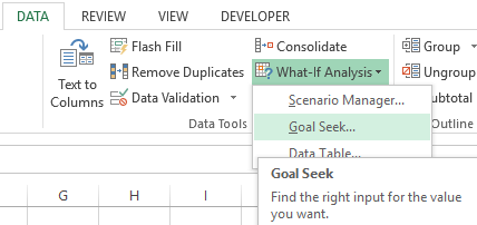
The path to the command: «DATA» — «Data Tools» — «What-if-Analysis» — «Goal Seek».
Let’s consider, for example, the solution of the quadratic equation x2 + 3x + 2 = 0. The order of finding the root with Excel:
- We enter into the cell B2 a formula for finding the value of the function. We apply a reference to cell B1 as an argument.
- Open the menu of the «Goal Seek» tool. In the box «Set cell» is a reference to cell B2 where the formula is located. Enter 0 in the «To value» field. This is the value that you want to get. In the column «By changing cell» is B1. The selected parameter should be displayed here.
- After clicking OK, the result of the selection is displayed. If you want to save it click OK again. Otherwise, click «Cancel».
The program uses a cyclic process to find a parameter. You need to enter the Excel parameters to change the number of iterations and the error.
Set the maximum number of iterations and the relative error on the «Formulas» tab. Set a checkmark in the box to enable iterative calculations.
How to solve the system of equations by using the matrix method in Excel?
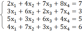
A system of equations is given:
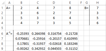
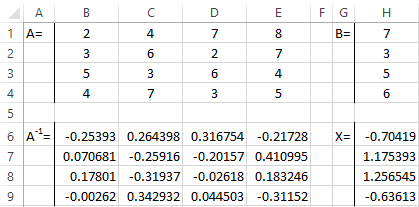
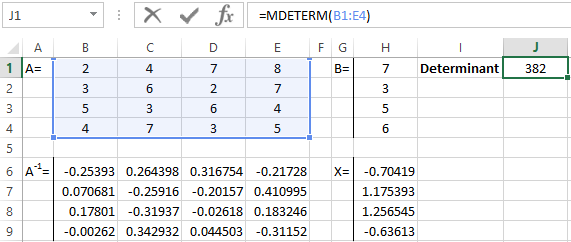
- We enter the values of the elements in Excel cells in the form of a table.
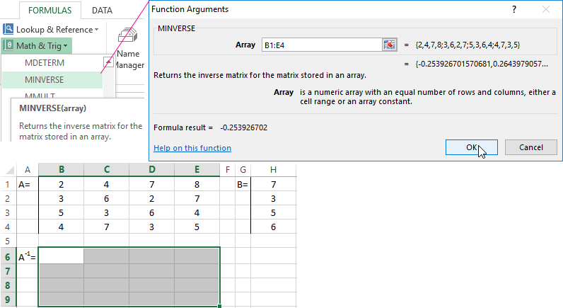
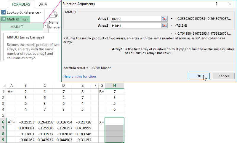
- Let us find the inverse matrix. Select the range B6:E9 where the matrix elements will later be placed (we are guided by the number of rows and columns in the original matrix). Open the list of functions (fx). In the category «Math and Trig» we find the MINVERS function. The argument is an array of cells with elements of the original matrix.
- Click OK and a value appears in the upper left corner of the range. Consecutively press the F2 button and Ctrl + Shift + Enter.
- We multiply the inverse matrix Ax-1x by the matrix B (only in this order of multiplication!). We select the range H1:H4 where the elements of the resulting matrix will subsequently appear (we are guided by the number of rows and columns of the matrix B). Open the dialog box of the MMULT mathematical function. The first range is the inverse matrix. The second one is the matrix B.
- Close the window with the arguments of the function by clicking OK. Consistently press the F2 button and the combination Ctrl + Shift + Enter.
The roots of the equations are obtained.
Solving the system of equations by the Cramer method in Excel
We take the system of equations from the previous example:
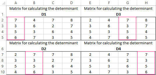
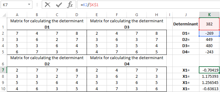
We calculate the determinants of the matrices obtained by replacing one column in the matrix A by the column matrix B. And it will be solved by using the Cramer method.
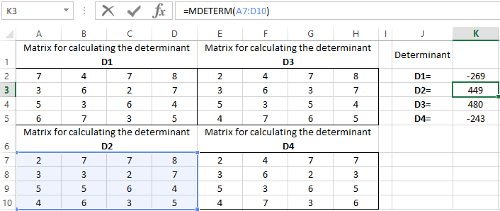
Use the MDETERM function to calculate the determinants. The argument is a range with the corresponding matrix.
We also calculate the determinant of the matrix A (the array is the range of the matrix A).
The determinant of the system is greater than 0 and the solution can be found by the Cramer formula (Dx / |A|).
For the calculation of Х1: =K2/$K$1, where K2 is D1. For the calculation of Х2: =K3/$K$1, and etc. We get the roots of the equations:
Solving the systems of equations by using the method of Gauss in Excel
For example, let’s take the simplest system of equations:
3а + 2в – 5с = -1
2а – в – 3с = 13
а + 2в – с = 9
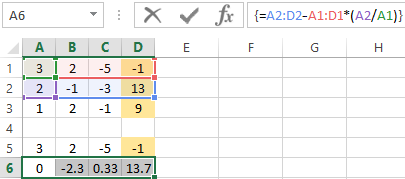
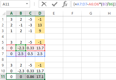
We write the coefficients in the matrix A. And write the constant term in the matrix B.
For clarity, the free terms will be selected by flood filling. You need to swap the lines if in the first cell of the matrix A was 0 so that there will be a value which differs from 0.
- We give the 0 to all the coefficients of the matrix A except the first equation. We copy the values in the first row of two matrices to cells B6:E6. In cell B7 we enter the formula:
Then select the range B7:E7. Press F2 and press Ctrl + Shift + Enter. We subtracted from the second line the first one which is multiplied by the ratio of the first elements of the second and first equation.
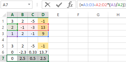
- Copy the entered formula on row 7. So we got rid of the coefficients before A. Only the first equation was retained.
- We reduce to 0 all the coefficients of B in the third and fourth equations. We copy lines 5 and 6 (only values). Then we transfer them below in lines 9 and 10. These data should remain unchanged. Then we enter the formula of the array in cell A11
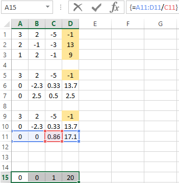
- A direct run was done by Gauss’s method. In the reverse order, we start running from the last row of the resulting matrix. All the elements of this line must be divided by a factor of C. Enter the array formula in the line:
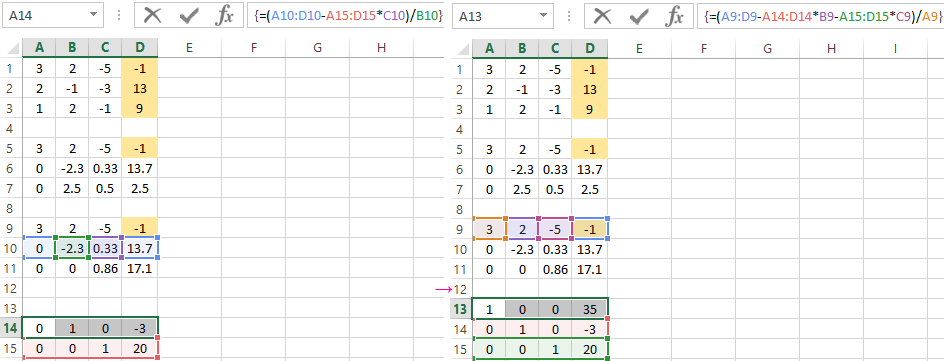
- In line 15: we subtract the third line from the second one, multiplied by the coefficient C from the second line
In line 14: from the first line we subtract the second and third one, multiplied by the corresponding coefficients
In the last column of the new matrix, we get the roots of the equation.
Examples of solving equations by using the iteration method in Excel
The calculations in the workbook should be configured as follows:
This can be done on the «Formulas» tab in the «Excel Options». Let’s find the root of the equation х – х3 + 1 = 0 (а = 1, b = 2) by iteration using cyclic references. Formula:
Хn+1 = Xn– F (Xn) / M, n = 0, 1, 2, … .
M is the maximum value of the derivative modulo. We perform the calculations to find M:
f’ (1) = -2 * f’ (2) = -11.
The resulting value is less than 0. Therefore, the function will have the opposite sign: f (х) = -х + х3 – 1. М = 11.
We enter the value in cell A1: a=1. Accuracy is three decimal places. Then we enter the formula to calculate the current value of x in an adjacent cell (B1):
We control the value of f(x) in cell C1 using the formula:
Download solving equations in Excel
The root of the equation is 1. We enter the value 2 into cell A1. We obtain the same result. There is only a single root in the given interval.
The Colebrook (or Colebrook-White) equation is the best way to dynamically determine the Darcy-Weisbach friction factor for turbulent pipe flow. The equations were developed via a curve fit to many experimental data points. In the post below, I demonstrate how to create a Colebrook equation solver in Excel.
Unfortunately, the equation is implicit (meaning that the friction factor, f, appears on both sides of the equation with no way to further simplify).
In order to find the friction factor, we need to solve the implicit equation using an iterative scheme. For this, we will use the Excel Goal Seek tool.
There are four variables in the equation:
- Darcy-Weisbach Friction Factor, f
- Roughness height, ε
- Hydraulic diameter, Dh
- Reynolds number, Re
Spreadsheet Inputs
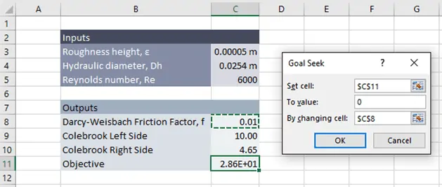
We will enter everything but f into the “Inputs” section of the spreadsheet.
Spreadsheet Outputs
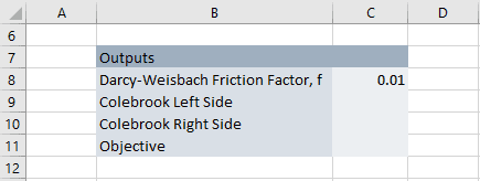
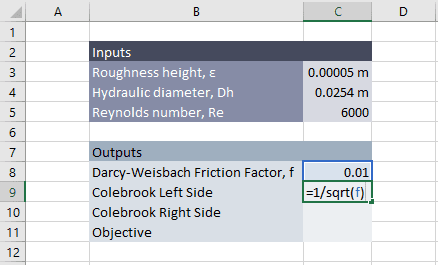
In the “Outputs” section of the spreadsheet we will create rows for the friction factor, left and right sides of the Colebrook equation, and an “Objective”.
In order for the Excel Goal Seek tool to work, we need to enter an initial guess value for the friction factor. Any small positive value should work. I chose 0.01.
We will use Goal Seek to find a value of f that minimizes the difference between the left and right sides of the Colebrook-White equation. Essentially, what we are looking for is the root of the equation. To do that we will calculate the left and right sides separately, then create an “Objective” function that we will attempt to minimize.
The left side of the equation is entered into cell C9 as follows (I used named ranges to make the equations clearer):
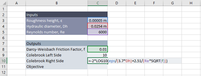
Similarly, the right side of the equation is entered into cell C10.
Iterative Solution using Excel Goal Seek
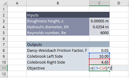
Before we can use Goal Seek to iterate to a solution for the friction factor, we need to define an Objective. We will set up Goal Seek to minimize this value (i.e. get it as close to zero as possible, within some tolerance).
The objective function must be set up such that it never returns a negative value, otherwise Excel will be sent into an unrecoverable tail spin.
To do this we will square the difference of the left and right hand sides of the equation.
Now we are ready to use the Goal Seek tool.
To access the Goal Seek tool, select Data>What-If Analysis>Goal Seek
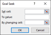
This opens up the Goal Seek window.
In words, what we are trying to do is: “Set the OBJECTIVE to a value of 0 by changing the FRICTION FACTOR”.
The way we do that in Excel is shown below:
Clicking “OK” returns the following:
The Goal Seek tool managed to drive the objective function to a value of 5.53E-04 (an acceptable level for our purposes), resulting in a friction factor of 0.0375.
We can check the result against a published Moody diagram to verify the calculation.
I would estimate the value on the Moody diagram at about ~0.038-0.039, so our result is pretty close (i.e. within approximately 5% at most).
Automating Goal Seek with VBA
What we have so far is nice, but it has a significant flaw.
Every time we update an input, we have to rerun Goal Seek again.
That means we have to navigate to the tool in the Ribbon, select the Friction Factor and Objective cells, and enter “0” for the goal value.
Blech.
What we would really like is to set this spreadsheet up so that the friction factor is updated automatically whenever an input value is changed.
Excel VBA can do this for us.
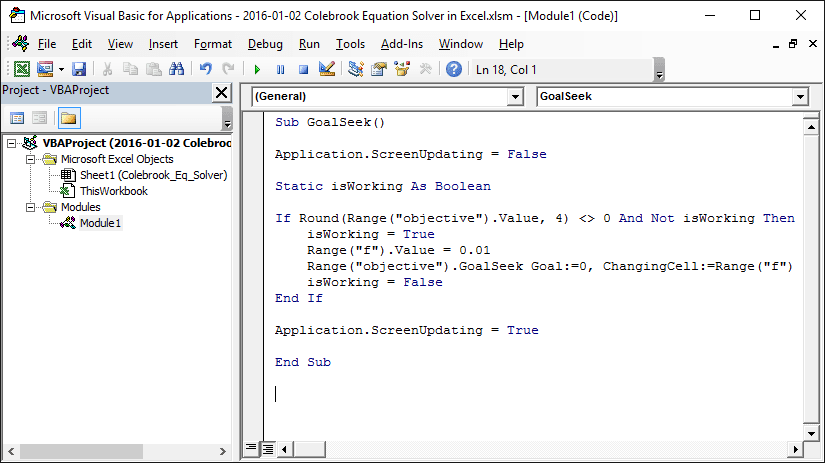
First we create a macro (in a new module) to run Goal Seek for us:
This macro does the following:
- Temporarily Disables Screen Updating
- Sets the value of “f” in Cell C8 to 0.01
- Runs Goal Seek if it is not currently running and the value of the objective cell round to 0 at 4 decimal places
- A Boolean (“isWorking”) that tells us whether or not Goal Seek is current running
- Enables Screen Updating
(Credit this site for the “isWorking” methodology.)
The macro automates setting up the Goal Seek, but it still has to be run manually.
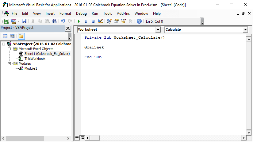
Let’s add some code to this worksheet (in the VBA editor) so that the macro runs every time there is a change to the worksheet (e.g. someone changes an input cell).
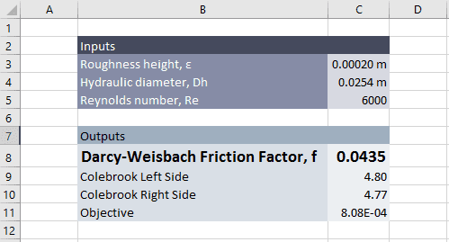
And, finally, let’s test it out:
I changed the roughness height to 0.0002 m, and the friction factor updated automatically.
Conclusion
So that’s how you create a Colebook equation solver in Excel. This method can be extended to tables of data to calculate pressure drop vs. flow in a pipe with a few tweaks to the VBA code. You can also use the Goal Seek method shown here for other iterative calculations in Excel.
Содержание
- Solver in Excel
- What is Solver in Excel?
- The Functioning of the Excel Solver
- How to add “Solver Add-In” in Excel?
- The Terminologies of the Solver in Excel
- The Types of Solving Methods
- How to use the Solver in Excel?
- Example #1
- Example #2
- The Applications of the Solver Excel Model
- Frequently Asked Questions
- Recommended Articles
- Solving equations in Excel using the Cramer and Gauss iterations method
- Solving equations by trial and error method in Excel
- How to solve the system of equations by using the matrix method in Excel?
- Solving the system of equations by the Cramer method in Excel
- Solving the systems of equations by using the method of Gauss in Excel
- Examples of solving equations by using the iteration method in Excel
Solver in Excel
What is Solver in Excel?
The solver in excel is an analysis tool that helps find solutions to complex business problems requiring crucial decisions to be made. For every problem, the goal (objective), variables, and constraints are identified. The solver returns an optimal solution which sets accurate values of the variables, satisfies all constraints, and meets the goal.
For example, the solver helps create the most appropriate project schedule, minimize an organization’s expenses on transportation of its employees, maximize the profits generated by a given marketing plan, and so on.
The solver can solve the following types of problems:
- Optimization problems where profits need to be maximized and costs need to be minimized
- Arithmetic equations
- Linear and nonlinear problems
Table of contents
The Functioning of the Excel Solver
For solving a problem, the user has to input certain parameters based on which the solver operates. The tasks of the user followed by the functions of the solver are listed as under:
- Identify the goal (objective) of the problem–This tells the solver what has to be done, thereby lending a direction to the solver.
- Choose the variables of the problem–This tells the solver the areas it has to work upon. The solver in excel returns the most appropriate values of the variables that meet the goal.
- Set the constraints of the problem–This tells the solver to work within the limits defined by the constraints. The solver returns a solution that meets the goal and, at the same time, does not go beyond these limitations.
Hence, the entire solution is focused on the goal of the problem. The solver returns the best possible solution for a problem keeping in mind the set of controls.
How to add “Solver Add-In” in Excel?
The “solver add-in” is not enabled by default in Excel. The two ways to activate the “add-in” are stated as follows:
a. With the “add-ins” option of the File menu
a. The steps under “add-ins” option of the File menu are listed as follows:
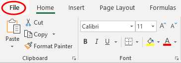
- Click on the File menu.
Select “options” from the various options listed in the menu.
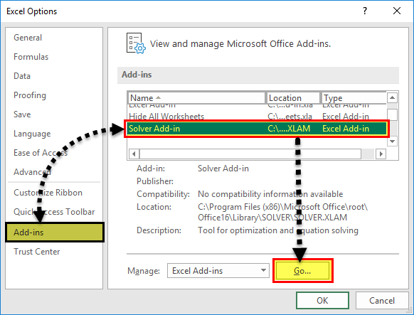
Click on “add-ins.” Select “solver add-in” and click “go.”
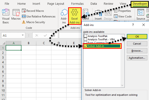
Select the checkbox for “solver add-in” and click “Ok.”
b. The steps under the Developer tab option are listed as follows:
- In the Developer tab, click on “Excel add-ins” in the “add-ins” group. Select the checkbox “solver add-in” and click “Ok.”
- Once installed, the “solver” button appears in the “analysis” group of the Data tab.
The Terminologies of the Solver in Excel
The solver model consists of the objective cells, variable cells, constraints, and formulas that interconnect these components. The excel solver finds an optimal solution to the formula mentioned in the objective cell by changing the variable data cells, given the restrictions of the constraint cells.
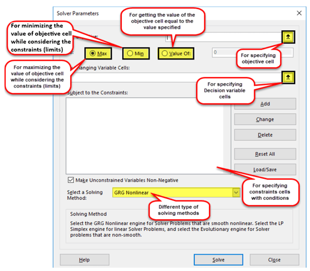
Let us understand the terminologies used in the “solver parameters” dialog box. This will be helpful when running the solver. The terms are defined as follows:
- Objective cell: This is a single cell which contains a formula. The formula is decision-based and subject to the restrictions of the constraint cells. The value of the objective cell can be minimized, maximized, or set equal to the specified target value.
- Decision variable or variable cells: These are the cells in which the solver returns the values based on the objective of the problem. Since these data cells are variable, they can be changed with respect to the objective. In Excel, up to 200 variable cells can be specified.
- Constraint cells: These are the limitations within which the given problem is solved. In other words, they are the conditions that should be satisfied.
The Types of Solving Methods
The three methods to solve the data in the excel solver are listed as follows:
- GRG nonlinear
The acronym “GRG” stands for “generalized reduced gradient nonlinear.” This method helps solve nonlinear problems. A nonlinear problem may have more than one feasible region. Alternatively, it may have a set of similar values for the variable cells with all the constraints being satisfied.
2. Simplex LP
The acronym “LP” stands for linear problems. This method helps solve linear programming problems and works faster than the GRG nonlinear method. In a linear programming problem, a single objective has to be maximized or minimized subject to certain conditions.
The simplex LP and GRG nonlinear method both are used for smooth problems.
3. Evolutionary
This method helps solve non-smooth problems, which consist of discontinuous functions. The non-smooth problems are the most challenging optimization models to solve.
How to use the Solver in Excel?
Let us consider some examples to understand the solver tool of Excel.
Example #1
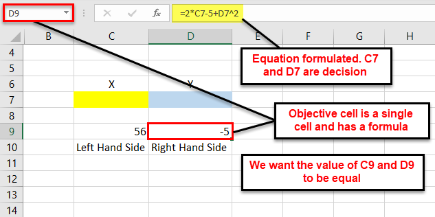
We want to find the value of X and Y in the following arithmetic equation with the help of the solver tool.
Step 1: Formulate the equation on an Excel sheet, as shown in the following image.
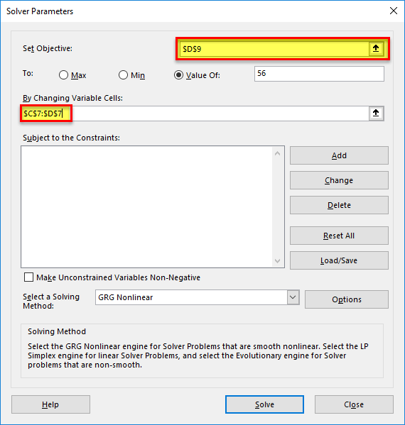
Step 2: Click the “solver” button in the “analysis” group of the Data tab. The “solver parameters” dialog box opens. Enter cell “$D$9” in the objective cell, as shown in the succeeding image. The variable cells are “$C$7:$D$7.”
In the “value of” box, type 56. This is because the right-hand side value of the given equation should be equal to 56.
Step 3: Select GRG nonlinear in the “select a solving method” box. Click “solve.”
Note: The GRG nonlinear is the default solving method.
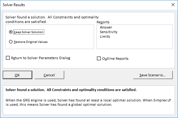
Step 4: The “solver results” box appears. This box may take some time to display depending on the complexity of the model. Select “keep solver solution” and click “Ok,” as shown in the following image.
Step 5: The results are shown in the following image. The solver has calculated X as 30.5 and Y as 0. The right-hand and left-hand sides both are equal now.
Example #2
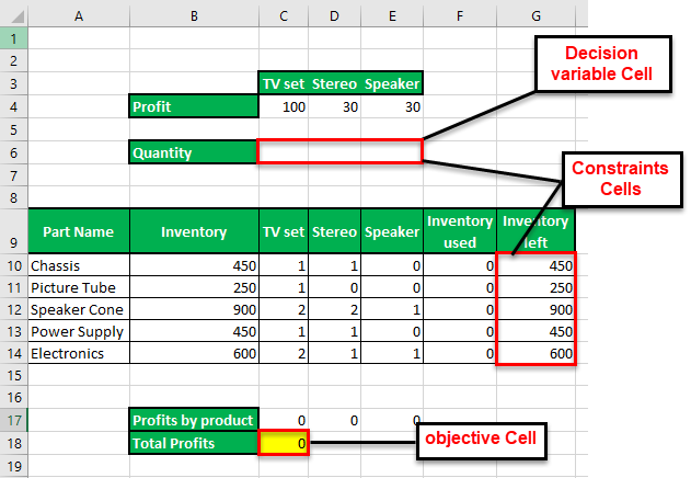
The succeeding image provides the details of an organization that manufactures a television set, stereo, and speaker. The raw materials used are chassis, picture tube, speaker cone, power supply, and electronics. The leftover stock of raw materials is given in G10:G14.
We want to maximize the overall profits given the limited availability of the raw materials.
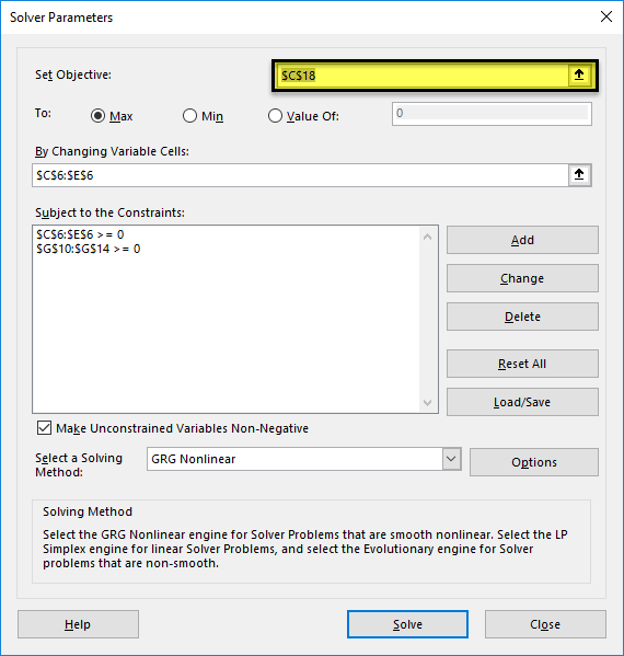
The variable cells, constraint cells, and the objective cell are highlighted.
Step 1: Calculate the “used inventory” in F10:F14. The formula is shown in the following image.
Step 2: Click the “solver” button in the “analysis” group of the Data tab. In the “solver parameters” dialog box, click “add” to the right of the “subject to the constraints” box.
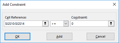
Step 3: The “add constraint” box appears, as shown in the succeeding image. The constraints are defined as follows:
- The leftover stock of raw materials should be greater than or equal to zero. So, enter “$G$10:$G$14” in the “ cell referenceCell ReferenceCell reference in excel is referring the other cells to a cell to use its values or properties. For instance, if we have data in cell A2 and want to use that in cell A1, use =A2 in cell A1, and this will copy the A2 value in A1.read more ” box. In the box to the right, type the comparison operator “>=.” In the “constraint” box, enter “0.”
- The quantity of the three products (television set, stereo, and speaker) should be greater than or equal to zero. So, enter “$C$6:$E$6>=0” as done for the preceding point.
After entering every constraint, click the “add” button to add it to the “solver parameters” box. Once all constraints have been entered, click “Ok.”
Step 4: In the “solver parameters” box, enter “$C$18” in the “set objective” box. Select the “max” option. In the “by changing variable cells” box, enter “$C$6:$E$6.” Select the solving method as GRG nonlinear. Click “solve.”
Step 5: The output is shown in the following image. The organization must produce 250 television sets, 50 stereos, and 50 speakers to make a profit of $28,000. The product-wise profits are also displayed in C17:E17.
This is an optimal solution given the constraints. With these numbers, the organization will be able to utilize its resources efficiently.
The Applications of the Solver Excel Model
The major applications of the excel solver are listed as follows:
- It helps take decisions at the top level of management. For instance, an organization may want to maximize the profits and minimize the costs given the limited resources of inventory and manpower.
- It helps solve the day-to-day problems of life which can be converted into arithmetic equations. For instance, a housewife may require an optimal monthly budget to be created which can meet the family’s financial needs, given the limitations.
Frequently Asked Questions
The solver can solve optimization problems, arithmetic equations, and linear and nonlinear programming models. It helps minimize or maximize the output based on the associated variables and the given constraints.
The solver tool consists of three components which are stated as follows:
• Objective cell – This contains a formula which is to be solved.
• Variable cells – These cells contain variable data which can be adjusted to attain the objective.
• Constraint cells – These are the conditions to be met by the solution of the problem.
The solver solves the problems with the help of three methods GRG nonlinear, simplex LP, and evolutionary. The first two methods are used for smooth problems, while the last helps solve non-smooth problems.
The objectives of using the solver are listed as follows:
• To find an optimal solution to a problem
• To help minimize or maximize the formula value
• To work on variable data provided the constraints are adhered to
• To perform a comprehensive analysis necessary for making decisions
The “solver parameters” is a dialog box which appears on clicking the “solver” button in the Data tab. It consists of the following components:
• “Set objective” – This is the objective cell categorized into “max,” “min,” and “value of.” The “max” and “min” help maximize or minimize the formula value respectively. The “value of” category helps set the desired target value.
• “By changing variable cells” – This consists of a range of variable data cells that are changed to achieve the goal.
• “Subject to the constraints” – These are the constraints that can be added, modified, and deleted depending on the requirement.
• “Load/save” button – This saves the current model and displays the stored parameters.
• “Select a solving method” – This consists of the method to solve the problem. Any one of the three methods (GRG nonlinear, simplex LP, and evolutionary) can be selected.
• “Solve” button – This is clicked once all the data has been entered in the tool. It takes the user to the “solver results” dialog box.
Note: If the variable cells are non-adjacent, select the range by pressing and holding the “Ctrl” key.
Recommended Articles
This has been a step-by-step guide to the Solver in Excel. Here we discuss how to use Solver in Excel along with examples and downloadable Excel templates. You may also look at these useful functions in Excel –
Источник
Solving equations in Excel using the Cramer and Gauss iterations method
There is an extensive toolkit in Excel for solving different types of equations by different methods. Let’s look at some solutions using examples.
Solving equations by trial and error method in Excel
The tool «Goal Seek» is used in a situation when the result is known but arguments are unknown. Excel picks up the values until the computation yields the desired total.
The path to the command: «DATA» — «Data Tools» — «What-if-Analysis» — «Goal Seek».
Let’s consider, for example, the solution of the quadratic equation x 2 + 3x + 2 = 0. The order of finding the root with Excel:
- We enter into the cell B2 a formula for finding the value of the function. We apply a reference to cell B1 as an argument.
- Open the menu of the «Goal Seek» tool. In the box «Set cell» is a reference to cell B2 where the formula is located. Enter 0 in the «To value» field. This is the value that you want to get. In the column «By changing cell» is B1. The selected parameter should be displayed here.
- After clicking OK, the result of the selection is displayed. If you want to save it click OK again. Otherwise, click «Cancel».
The program uses a cyclic process to find a parameter. You need to enter the Excel parameters to change the number of iterations and the error.
Set the maximum number of iterations and the relative error on the «Formulas» tab. Set a checkmark in the box to enable iterative calculations.
How to solve the system of equations by using the matrix method in Excel?
A system of equations is given:
- We enter the values of the elements in Excel cells in the form of a table.
- Let us find the inverse matrix. Select the range B6:E9 where the matrix elements will later be placed (we are guided by the number of rows and columns in the original matrix). Open the list of functions (fx). In the category «Math and Trig» we find the MINVERS function. The argument is an array of cells with elements of the original matrix.
- Click OK and a value appears in the upper left corner of the range. Consecutively press the F2 button and Ctrl + Shift + Enter.
- We multiply the inverse matrix Ax -1x by the matrix B (only in this order of multiplication!). We select the range H1:H4 where the elements of the resulting matrix will subsequently appear (we are guided by the number of rows and columns of the matrix B). Open the dialog box of the MMULT mathematical function. The first range is the inverse matrix. The second one is the matrix B.
- Close the window with the arguments of the function by clicking OK. Consistently press the F2 button and the combination Ctrl + Shift + Enter.
The roots of the equations are obtained.
Solving the system of equations by the Cramer method in Excel
We take the system of equations from the previous example:
We calculate the determinants of the matrices obtained by replacing one column in the matrix A by the column matrix B. And it will be solved by using the Cramer method.
Use the MDETERM function to calculate the determinants. The argument is a range with the corresponding matrix.
We also calculate the determinant of the matrix A (the array is the range of the matrix A).
The determinant of the system is greater than 0 and the solution can be found by the Cramer formula (Dx / |A|).
For the calculation of Х1: =K2/$K$1, where K2 is D1. For the calculation of Х2: =K3/$K$1, and etc. We get the roots of the equations:
Solving the systems of equations by using the method of Gauss in Excel
For example, let’s take the simplest system of equations:
3а + 2в – 5с = -1
2а – в – 3с = 13
а + 2в – с = 9
We write the coefficients in the matrix A. And write the constant term in the matrix B.
For clarity, the free terms will be selected by flood filling. You need to swap the lines if in the first cell of the matrix A was 0 so that there will be a value which differs from 0.
- We give the 0 to all the coefficients of the matrix A except the first equation. We copy the values in the first row of two matrices to cells B6:E6. In cell B7 we enter the formula: Then select the range B7:E7. Press F2 and press Ctrl + Shift + Enter. We subtracted from the second line the first one which is multiplied by the ratio of the first elements of the second and first equation.
- Copy the entered formula on row 7. So we got rid of the coefficients before A. Only the first equation was retained.
- We reduce to 0 all the coefficients of B in the third and fourth equations. We copy lines 5 and 6 (only values). Then we transfer them below in lines 9 and 10. These data should remain unchanged. Then we enter the formula of the array in cell A11
- A direct run was done by Gauss’s method. In the reverse order, we start running from the last row of the resulting matrix. All the elements of this line must be divided by a factor of C. Enter the array formula in the line:
- In line 15: we subtract the third line from the second one, multiplied by the coefficient C from the second line In line 14: from the first line we subtract the second and third one, multiplied by the corresponding coefficients In the last column of the new matrix, we get the roots of the equation.
Examples of solving equations by using the iteration method in Excel
The calculations in the workbook should be configured as follows:
This can be done on the «Formulas» tab in the «Excel Options». Let’s find the root of the equation х – х 3 + 1 = 0 (а = 1, b = 2) by iteration using cyclic references. Formula:
M is the maximum value of the derivative modulo. We perform the calculations to find M:
f’ (1) = -2 * f’ (2) = -11.
The resulting value is less than 0. Therefore, the function will have the opposite sign: f (х) = -х + х 3 – 1. М = 11.
We enter the value in cell A1: a=1. Accuracy is three decimal places. Then we enter the formula to calculate the current value of x in an adjacent cell (B1):
We control the value of f(x) in cell C1 using the formula:
The root of the equation is 1. We enter the value 2 into cell A1. We obtain the same result. There is only a single root in the given interval.
Источник
Возможно вы слышали о нобелевском лауреате, психологе и исследователе по имени Дэниель Канеман. Канеман занимался наукой, которую называют термином «поведенческая экономика», т.е. изучал реакции, поведение и суждения людей в типовых жизненных (и экономических) ситуациях и условиях неопределенности.
В его книге, которая называется «Думай медленно — решай быстро» (очень рекомендую, кстати) в качестве одного из примеров когнитивных искажений — несознательной автоматической реакции — приводится следующая задача:
Бейсбольная бита и мяч стоят вместе 1 доллар 10 центов.
Бита дороже мяча на 1 доллар.
Сколько стоит мяч?
Подозреваю, что вашей первой рефлекторной мыслью, скорее всего, будет «10 центов!» 
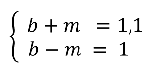
Конечно можно «тряхнуть стариной» и решить всё вручную на бумажке через подстановку переменных — как-то так:
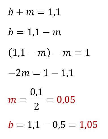
Но, во-первых, на практике уравнения могут быть сложнее и переменных может оказаться сильно больше двух и, во-вторых, у нас с вами есть Microsoft Excel — универсальный мега-инструмент, величайшее изобретение человечества. Так что давайте-ка лучше разберём как решить нашу задачу с его помощью.
Способ 1. Матричные функции МУМНОЖ и МОБР
Само собой, изобретать велосипед тут не надо — прогрессивное человечество в лице математиков давным-давно придумало кучу способов для решения подобных задач. В частности, если уравнения в нашей системе линейные (т.е. не используют степени, логарифмы, тригонометрические функции типа sin, cos и т.д.), то можно использовать метод Крамера.
Сначала записываем числовые коэффициенты, стоящие перед нашими переменными в виде матрицы (в нашем случае — размером 2х2, в общем случае — может быть и больше).
Затем находим для неё так называемую обратную матрицу , т.е. матрицу, при умножении которой на исходную матрицу коэффициентов получается единица. В Excel это легко сделать с помощью стандартной математической функции МОБР (MINVERSE):
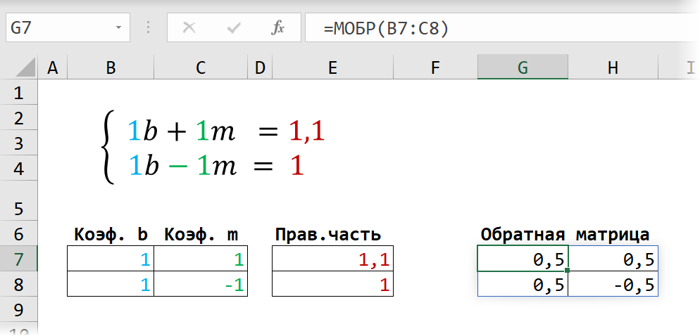
Здесь важно отметить, что если у вас свежая версия Excel 2021 или Excel 365, то достаточно ввести эту функцию обычным образом в первую ячейку (G7) — сразу получится динамический массив с обратной матрицей 2х2. Если же у вас более старая версия Excel, то эту функцию нужно обязательно вводить как формулу массива, а именно:
- Выделить диапазон для результатов — G7:H8
- Ввести функцию =МОБР(B7:C8) в строку формул
- Нажать на клавиатуре сочетание клавиш Ctrl+Shift+Enter
Замечательное свойство обратной матрицы состоит в том, что если умножить её на значения правых частей наших уравнений (свободные члены), то мы получим значения переменных, при которых левые и правые части уравнений будут равны, т.е. решения нашей задачи. Выполнить такое матричное умножение можно с помощью ещё одной стандартной экселевской функции МУМНОЖ (MMULT):
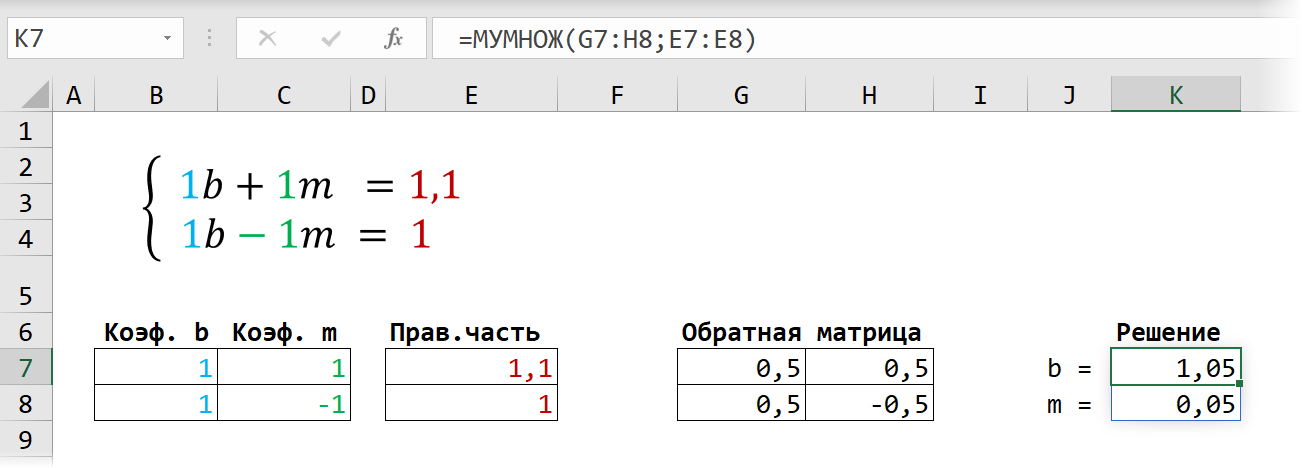
Если у вас старая версия Excel, то не забудьте также ввести её в режиме формулы массива, т.е. сначала выделить диапазон K7:K8, а после ввода функции нажать сочетание клавиш Ctrl+Shift+Enter.
Само собой, уравнений и переменных может быть больше, да и посчитать всё можно сразу в одной формуле, вложив используемые функции одна в другую:
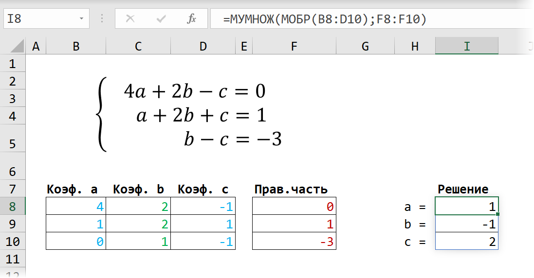
Не так уж и сложно, правда? Однако надо понимать, что этот метод подходит только для решения систем линейных уравнений. Если у вас в уравнениях используются функции посложнее четырех базовых математических действий, то зачастую проще будет пойти другим путем — через подбор.
Способ 2. Подбор надстройкой «Поиск решения» (Solver)
Принципиально другой способ решения подобных задач — это итерационные методы, т.е. последовательный подбор значений переменных, чтобы после подстановки их в наши уравнения мы получили верные равенства. Само собой, подбор имеется ввиду не тупой и долгий (брутфорс), а умный и быстрый, благо математики, опять же, давным-давно придумали кучу различных методов для решения таких задач буквально за несколько итераций.
В Microsoft Excel некоторые из этих методов реализованы в стандартной надстройке Поиск решения (Solver). Её можно подключить через Файл — Параметры — Надстройки — Перейти (File — Options — Add-ins — Go to) или на вкладке Разработчик — Надстройки (Developer — Add-ins).
Давайте рассмотрим её использование на следующей задаче. Предположим, что нам с вами нужно решить вот такую систему из двух нелинейных уравнений:

Подготавливаем основу для оптимизации в Excel:
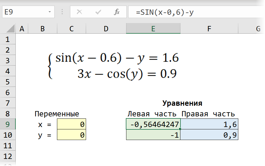
Здесь:
- В жёлтых ячейках C9:C10 лежат текущие значения наших переменных, которые и будут подбираться в процессе оптимизации. В качестве стартовых можно взять любые значения, например, нули или единицы — роли не играет. Для удобства, кстати, этим ячейкам можно дать имена, назвав их именами переменных x и y, — для этого выделите диапазон C9:C10 и выберите команду Формулы — Создать из выделенного — Слева (Formulas — Create from selection — Left column).
- В зелёных ячейках E9:E10 введены наши уравнения с использованием либо прямых ссылок на жёлтые ячейки переменных, либо созданных имён (так нагляднее). В результате мы видим, чему равны наши уравнения при текущих значениях переменных.
- В синих ячейках F9:F10 введены значения правых частей наших уравнений, к которым мы должны стремиться.
Теперь запускаем нашу надстройку на вкладке Данные — Поиск решения (Data — Solver) и вводим в появившемся диалоговом окне следующие параметры:
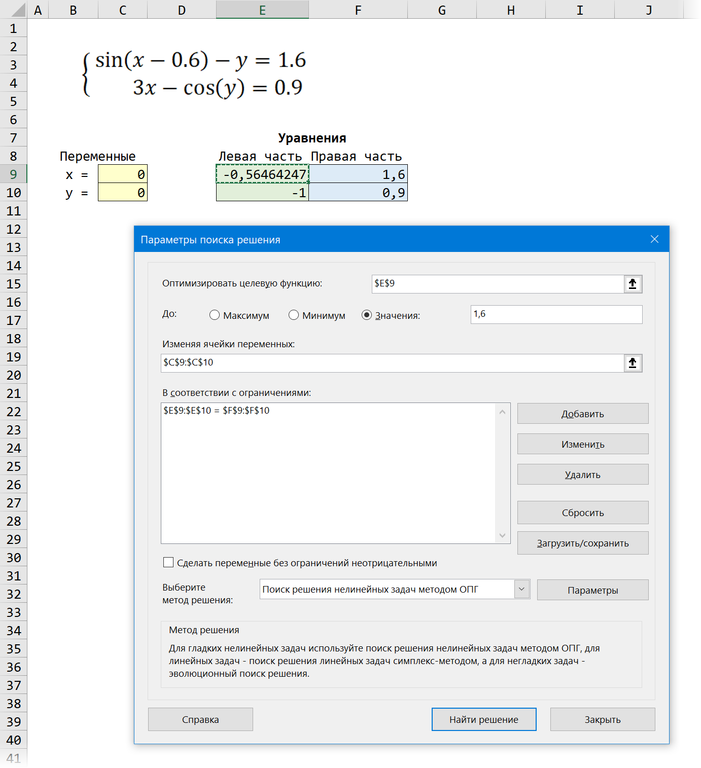
- Оптимизировать целевую функцию (Set target cell) — любая из двух наших зелёных ячеек с уравнениями, например E9.
- Изменяя ячейки переменных (By changing cells) — жёлтые ячейки с текущими значениями переменных, которыми мы «играем».
- Добавляем ограничение с помощью кнопки Добавить (Add) и задаём равенство левой и правой части наших уравнений, т.е. зелёного и голубого диапазонов.
- В качестве метода решения выбираем Поиск решения нелинейных задач методом ОПГ, т.к. уравнения у нас нелинейные. Для линейных можно смело выбирать симплекс-метод.
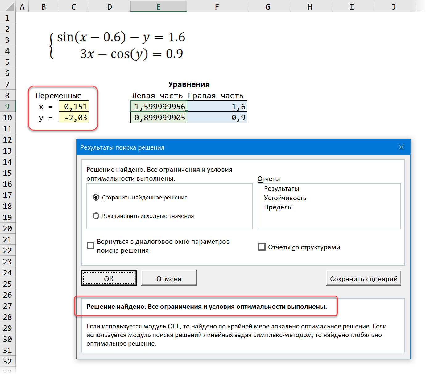
После нажатия на кнопку Найти решение (Solve) через пару мгновений (или не пару — это зависит от сложности задачи) мы должны увидеть окно с результатами. Если решение найдено, то в жёлтых ячейках отобразятся подобранные значения наших переменных:
Обратите внимание, что поскольку мы здесь используем итерационные, а не аналитические методы, то зеленые ячейки не совсем равны голубым, т.е. найденное решение не абсолютно точно. На практике, конечно же, такой точности вполне достаточно для большинства задач, и если необходимо, её можно настроить, вернувшись в окно Поиск решения и нажав кнопку Параметры (Options).
Solve Equation in Excel (Table of Contents)
- Overview of Solve Equation in Excel
- How to Add the Solver Add-in Tool?
- Example on How to Solve Equations Using Solver Add-in Tool
Overview of Solve Equation in Excel
Excel help’s us out in many ways by making the task easier & simple. Solver Add-in tool is significant to perform or solve equations in excel. Sometimes we need to perform or carry out reverse calculations, where we need to calculate one or two variables to get the desired end results.
Example: For the profit of the extra 10%, how many units need to be sold or what is the exact marks needed in the last semester of final exams to get the distinction.
This above calculation or equations can be calculated with the help of Solver Add-in, with specific criteria.
Definition of Solve Equation in Excel
It is used to determine the optimal value of the target cell by changing values in cells used to calculate the target cell.
It contains the below-mentioned parameters.
- Target
- Variables
- Constraints
- Formula to use to calculate
How to Add the Solver Add-in Tool?
Let’s check out how to add the solver add-in tool in excel. Calculation or equations can be calculated with the help of Solver Add-in, with specific criteria.
To add the Solver Add-in tool, the below-mentioned procedure is followed:
- Click on the File option or an Office Button; then, you need to click on Excel Options.
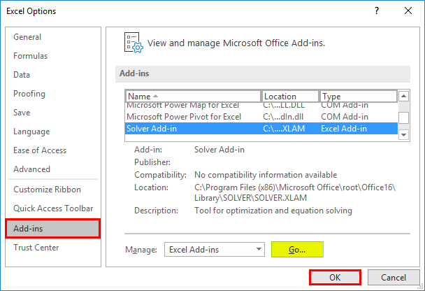
- Now, the Excel Options window dialog box appears; under Add-ins, select Solver Add-in in the inactive application add-ins list and “Go.”
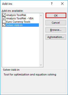
- Add-ins window appears where you can see the list of active add-ins options. Tick the Solver Add-in and click on the “Ok” button.
Now, you can observe, Solver Add-in got added to the Excel sheet as Solver under the “Data” tab on the extreme right side.
Example on How to Solve Equations Using Solver Add-in Tool
To calculate Variable Values For % Profit Maximization with the help of the Solver Add-in Tool.
You can download this Solve Equation Excel Template here – Solve Equation Excel Template
In the above-mentioned table, the monthly sales data of price per unit, containing Cost or stockiest Price per unit & Selling Price per unit to customers. Now, I have April & May month with a percentage profit for each unit, i.e. 13.33% & 15.38% respectively.
Here, B4 & C4 is the percentage profit for the month of April & May 2019, which is calculated with the help of the below-mentioned formula.
Formula to Find out Percentage Profit:
((Selling price per unit – Stockist price per unit)/ Stockist price per unit) *100
Variables (B2, B3 & C2, C3): Here, variables are Cost or stockiest Price per unit & Selling Price per unit to customers, which keeps on changing month on month.
Target & Constraints
Now, my target is to take the percentage profit (%) per unit to 20%. So, for that, I need to find out the Cost or stockiest Price per unit & Selling Price per unit to customers needed to achieve a profit of 20%.
- Target Cell: D4 (Profit %) should give a 20% profit
- Variable Cells: C2 (Cost or stockiest Price per unit) and C3 (Selling Price per unit to customers)
- Constraints: D2 should be >= 16,000 and D3 should be <= 20,000
Formula to Find out Percentage Profit:
((Selling price per unit – Stockist price per unit)/ Stockist price per unit) *100
i.e. ((D3-D2)/D2) *100
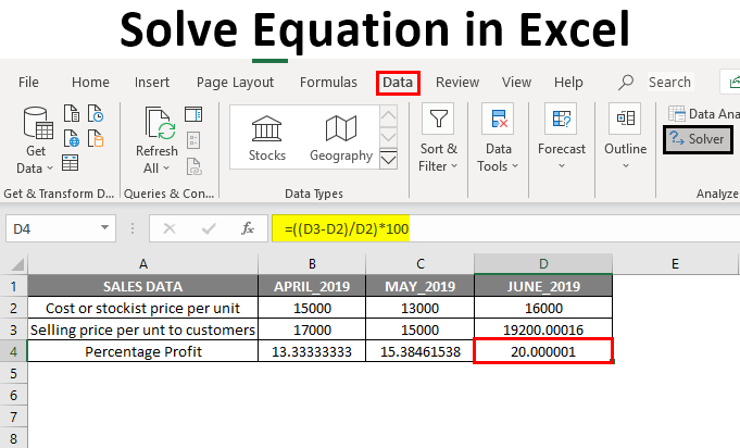
Prior to usage of the solver add-in tool, we need to enter the profit calculator formula ((D3-D2)/D2) *100 in the target cell (D4) to calculate the 20 % profit.
It is the significant information which is required to solve any sort of equation using Solver Add-in in Excel. Now, select a cell D4, and I need to launch the Solver Add-in by clicking on the Data tab and select a Solver.
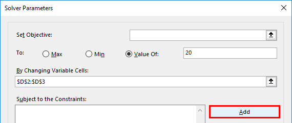
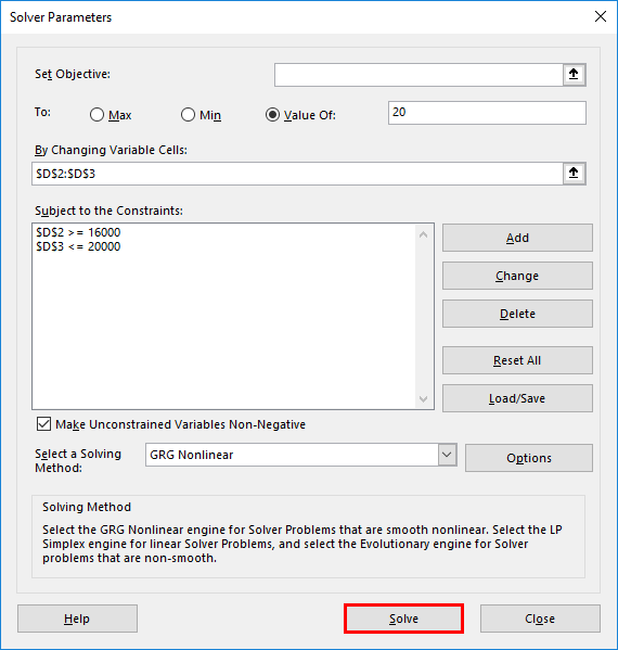
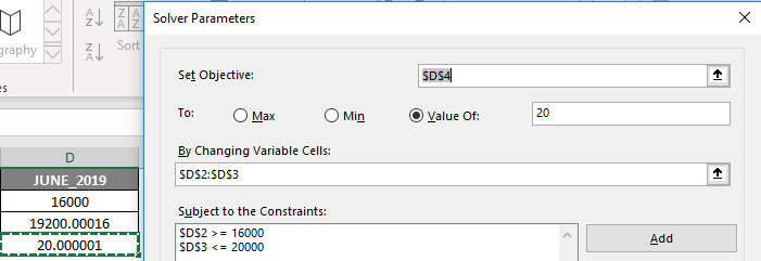
Once solver is selected, Solver parameter window appears, where you need to mention the “Target Cell” as “D4” cell reference in the set objective text box and select a radio button as “Value of”, In the text box of it set the targeted profit as 20 %
In the “By changing variable cells”, select the range of D2 (Cost or stockiest Price per unit) and D3 (Selling Price per unit to customers) cell where it is mentioned as $D$2:$D$3 in the text box.
After the addition of changing variable cell range, we need to add constraints; it is added by clicking on add under the subject to the constraints.
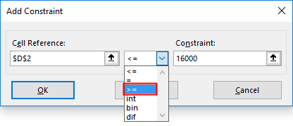
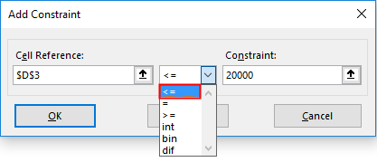
Now, the first parameter of Constraints is added by inputting the cell reference & constraint value, i.e. Cost price or stockiest Price per unit, which is either more than or equal to 16,000 (>=16000)
Now it gets reflected under Subject to the Constraints box, again we need to click on add to add one more constraint, i.e. Selling Price per unit to customers, it is added by inputting the cell reference & constraint value, which is either less than or equal to 20,000 (<=20000)
Now, we added all the parameters; just we need to click on solve.
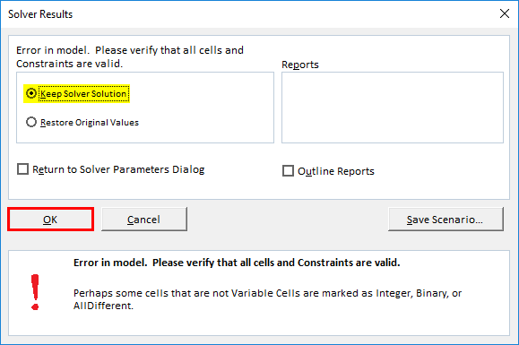
It will ask whether you want to keep the solver solution along with original values; you can Select these options based on your requirement; here, in this scenario, I have selected Keep Solver Solution and click on the “Ok” button.
Now, you will observe a change in the value in the cell D2 (Cost or stockiest Price per unit) and D3 (Selling Price per unit to customers) to 16000 and 19200 respectively to get the 20% Profit.
Things to Remember About Solve Equation in Excel
Most of the third party excel add-in program is available, that provides to solve equations & data analysis tools for statistical, financial and engineering data and Other tools & function which are used to solve equations in excel are:
- What-If Analysis: It is also used to solve equations & data analysis, wherein it allows you to try out different values (scenarios) for formulas to get the desired output.
- Goal Seek: It is an inbuilt function in excel under What-If Analysis, which helps us solve equations to source cell values until the desired output is achieved.
Recommended Articles
This is a guide to Solve Equation in Excel. Here we discuss how to add the Solver Add-in Tool and how to Solve equations with Solver Add-in Tool in excel. You can also go through our other suggested articles to learn more –
- Evaluate Formula in Excel
- Excel Solver Tool
- VBA Solver
- Standard Deviation in Excel

