Equation from graph excel

How to Graph an Equation / Function – Excel & Google Sheets

This tutorial will demonstrate how to graph a Function in Excel & Google Sheets.

How to Graph an Equation / Function in Excel

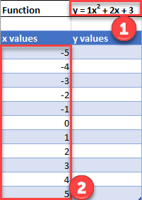
Set up your Table

1. Create the Function that you want to graph
2. Under the X Column, create a range. In this example, we’re range from -5 to 5

Fill in Y Column

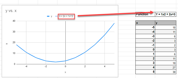
Create a formula using the Function, substituting x with what is in Column B.

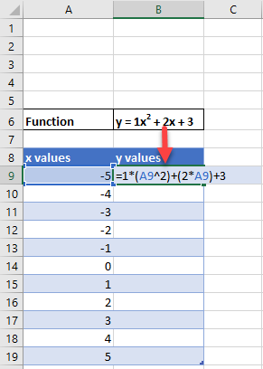
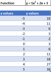
After using this formula for all the rows, you should have a table that looks like below.

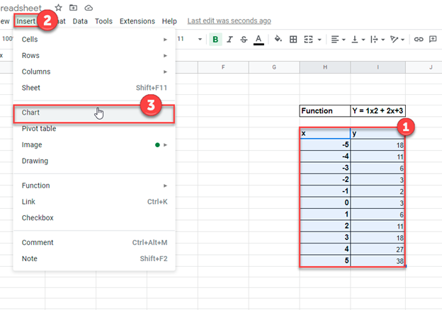
Creating Scatterplot

1. Highlight Dataset
2. Select Insert
3. Select Scatterplot
4. Select Scatter with Smooth Lines

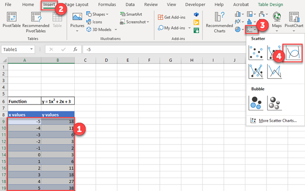
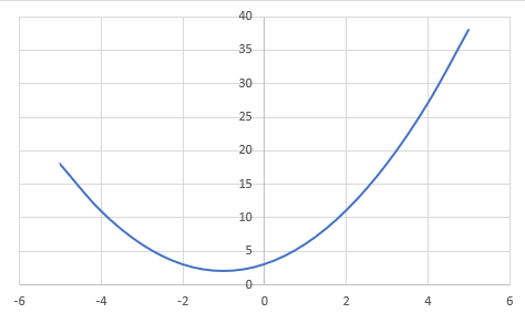
This will create a graph that should look similar to below.

Add Equation Formula to Graph

1. Click Graph
2. Select Chart Design
3. Click Add Chart Element
4. Click Trendline
5. Select More Trendline Options

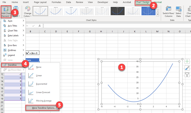
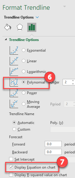
6. Select Polynomial

7. Check Display Equation on Chart

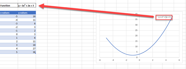
Final Scatterplot with Equation

Your final equation on the graph should match the function that you began with.

How to Graph an Equation / Function in Google Sheets

Creating a Scatterplot

1. Using the same table that we made as explained above, highlight the table
2. Click Insert
3. Select Chart

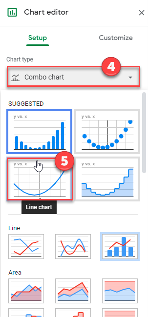
4. Click on the dropdown under Chart Type

5. Select Line Chart

Adding Equation

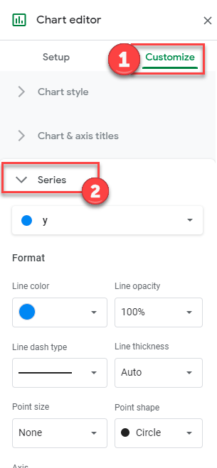
1. Click on Customize
2. Select Series

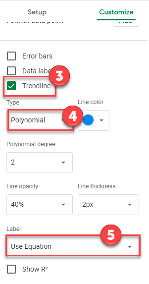
3. Check Trendline

4. Under Type, Select Polynomial

5. Under Label, Select Use Equation

Final Scatterplot with Equation

As you can see, similar to the exercise in Excel, the equation matches the function that we began with.

Источник

How to add equation to graph – Excelchat

We can add an equation to a graph in excel by using the excel equation of a line . Graph equations in excel are easy to plot and this tutorial will walk all levels of excel users through the process of showing line equation and adding it to a graph .

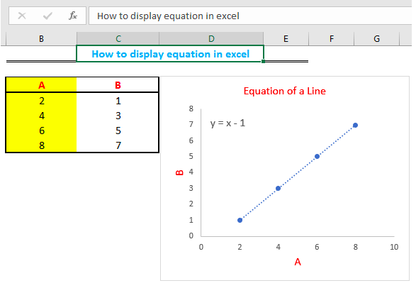Figure 1: Graph equation

Tabulate Data

• We will tabulate our data in two columns.

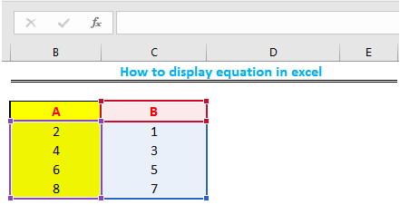Figure 2: Table of Data

• We will then highlight our entire table and click on “insert ”, then we will then select the “scatter chart” icon to display a graph

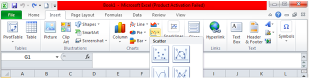Figure 3 – Scatter chart

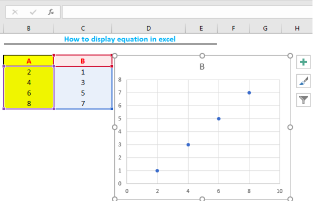Figure 4: Graphical Representation of Data

• We will now click on the “+” icon beside the chart to edit our graph by including the Chart Title and Axes. We will also remove the gridlines.

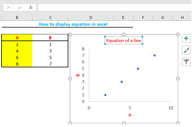Figure 5: Edited Graph Parameters

• We will now add the equation of the chart by right clicking on any of the point on the chart, select “add trendline” , then scroll down and finally select “Display Equation on Chart” .

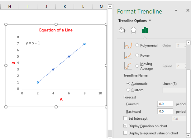Figure 6: Equation of a line

Instant Connection to an Expert through our Excelchat Service

Most of the time, the problem you will need to solve will be more complex than a simple application of a formula or function. If you want to save hours of research and frustration, try our live Excelchat service! Our Excel Experts are available 24/7 to answer any Excel question you may have. We guarantee a connection within 30 seconds and a customized solution within 20 minutes.

Источник

How to Fit an Equation to Data in Excel

You can use Excel to fit simple or even complex equations to data with just a few steps.

Determine the Form of the Equation

The first step in fitting an equation to data is to determine what form the equation should have. Sometimes this is easy, but other times it will be more difficult. Usually, the equation you choose will come from prior knowledge of the system you are analyzing.

Either way, it all starts with inspecting the data, and the easiest way to do that is to plot it in a chart. I’ve done that with some sample data below, and it’s obvious that we can fit a quadratic function to this data. Regardless of the complexity of the function, the method I’ll be showing is still valid. I’ve just chosen a simple example for this demonstration.

Once you’ve determined the form the equation should have, the next step is to define the parameters for the equation. Assuming the y-intercept is 0, a quadratic equation has the form:

so, our parameters are a and b.

We can input arbitrary values for those parameters on our spreadsheet. The values that are entered don’t matter for now because we’ll be adjusting them later to fit the function to the data.

Calculate the Equation from the Parameters

Next, we calculate a new series in Excel using the equation above. The series will be a function of the parameters a and b, and the independent variable, x.

Plotting the original y-data and the calculated result, “ycalc”, on the same graph tells us that the parameters of the function are not yet correct. But we will fix that soon by adjusting them to find the best fit.

Calculate the Sum of Residuals Squared

Although it would be tedious, we could manually adjust the two parameters and “eyeball” the curve fit until it looked good. But we’re smarter than that, so we’ll use the method of least squares along with Solver to automatically find the parameters that define the best fit curve much more efficiently.

Solver works by optimizing a single objective cell, so we’ll need to create an output that defines how well the function fits the data. This output is the sum of the residuals squared.

Residuals are the difference between the value provided by the function and the data value at a given value of x.

So, let’s create another column for the residuals:

Then, to calculate the sum of the residuals squared, use the SUMSQ function:

Minimizing this term will let us know that we have found the parameters that best fit the function to the data. To minimize this term, we’ll use Solver.

Find the Best-Fit Parameters

If you haven’t already activated the Solver add-in in your copy of Excel, you can find instructions to do that right here.

Once installed, you can open it from the far-right side of the Data tab:

With Solver open, select the cell that contains the SUMSQ formula as the objective, and the cells containing the values for “a” and “b” as the variable cells.

The goal, of course, is to minimize the sum of the residuals squared, so select the button next to “Min” in the Solver window.

Finally, uncheck the box next to “Make unconstrained variables non-negative.” We don’t know beforehand that the best values of a and b are necessarily positive, so this constraint is invalid.

For my worksheet, the Solver window has the following setup:

For a simple model like this, it’s not necessary to change any of the solver options. However, for more complex equations that may be necessary, and I’ve explained how to do so in this post.

All that’s left now is to click “Solve” and let Solver find the optimum parameters for the function.

Check the Result

Solver adjusts the values of the constants until the sum of the squared residuals is minimized. Those values are shown below:

The magnitude of the minimized sum of squared residuals is relative and depends on the data you are working with. Smaller data values are going to result in a smaller sum of squared residuals than larger values.

Finally, we can check the fit of the equation to the data by plotting both on the same chart. In the chart below, the orange circles are the function and the blue circles are the underlying data from which the function was derived.

Are you struggling to the find the right solutions to your engineering problems in Excel?

In Engineering with Excel, you’ll learn Excel for advanced engineering calculations through a step-by-step system that helps engineers solve difficult problems quickly and accurately.

Источник

How to Make a Graph in Excel & Add Visuals to Your Reporting

Most companies (and people) don’t want to pore through pages and pages of spreadsheets when it’s so quick to turn those rows and columns into a visual chart or graph. But someone has to do it…and that person must be you.

Ready to turn your boring Excel spreadsheet into something a little more interesting?

In Excel, you’ve got everything you need at your fingertips. Excel users can leverage the power of visuals without any additional extensions. You can create a graph or chart right inside Excel rather than exporting it into some other tool.

What is the difference between Charts and Graphs?

According to reference.com…“The difference between graphs and charts is mainly in the way the data is compiled and the way it is represented. Graphs are usually focused on raw data and showing the trends and changes in that data over time. Charts are best used when data can be categorized or averaged to create more simplistic and easily consumed figures.“

So technically, charts and graphs mean separate things, but in the real world, you’ll hear the terms used interchangeably. People generally accept both so don’t worry too much about it!

In this post, you’ll learn exactly how to create a graph in Excel and improve your visuals and reporting…but first let’s talk about charts. Understanding exactly how charts play out in Excel will help with understanding graphs in Excel.

Charts in Excel

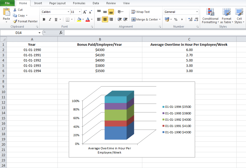
Charts are usually considered more aesthetically pleasing than graphs. Something like a pie chart is used to convey to readers the relative share of a particular segment of the data set with respect to other segments that are available. If instead of the changes in hours worked and annual leaves over 5 years, you want to present the percentage contributions of the different types of tasks that make up a 40 hour work week for employees in your organization then you can definitely insert a pie chart into your spreadsheet for the desired impact.

Graphs in Excel

Graphs represent variations in values of data points over a given duration of time. They are simpler than charts because you are dealing with different data parameters. Comparing and contrasting segments of the same set against one another is more difficult.

So if you are trying to see how the number of hours worked per week and the frequency of annual leaves for employees in your company has fluctuated over the past 5 years, you can create a simple line graph and track the spikes and dips to get a fair idea.

Types of Graphs Available in Excel

Excel offers three varieties of graphs:

• Line Graphs: Both 2 dimensional and three dimensional line graphs are available in all the versions of Microsoft Excel. Line graphs are great for showing trends over time. Simultaneously plot more than one data parameter – like employee compensation, average number of hours worked in a week and average number of annual leaves against the same X axis or time.
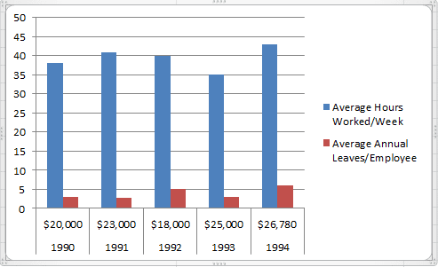
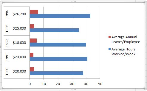
• Column Graphs: Column graphs also help viewers see how parameters change over time. But they can be called “graphs” when only a single data parameter is used. If multiple parameters are called into action, viewers can’t really get any insights about how each individual parameter has changed. As you can see in the Column graph below, average numbers of hours worked in a week and average number of annual leaves when plotted side by side do not provide the same clarity as the Line graph.

• Bar Graphs: Bar graphs are very similar to column graphs but here the constant parameter (say time) is assigned to the Y axis and the variables are plotted against the X axis.

How to Make a Graph in Excel

1. Fill the Excel Sheet with Your Data & Assign the Right Data Types

The first step is to actually populate an Excel spreadsheet with the data that you need. If you have imported this data from a different software, then it’s probably been compiled in a .csv (comma separated values) formatted document.

If this is the case, use an online CSV to Excel converter like the one here to generate the Excel file or open it in Excel and save the file with an Excel extension.

After converting the file, you still may need to clean up the rows and the columns. It is better to work with a clean spreadsheet so that the Excel graph you’re creating is clean and easy to modify or change.

If that doesn’t work, you may also need to manually enter the data into the spreadsheet or copy and paste it over before creating the Excel graph.

Excel has two components to its spreadsheets:

• The rows that are horizontal and marked with numbers
• The columns that are vertical and marked with alphabets

After all the data values have been set and accounted for, make sure that you visit the Number section under the Home tab and assign the right data type to the various columns. If you do not do this, chances are your graphs will not show up right.

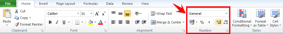
For example if column B is measuring time, ensure that you choose the option Time from the drop down menu and assign it to B.

Choose the Type of Excel Graph You Want to Create

This will depend on the type of data you have and the number of different parameters you will be tracking simultaneously.

If you are looking to take note of trends over time then Line graphs are your best bet. This is what we will be using for the purpose of the tutorial.
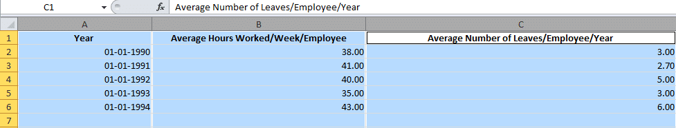
Let us assume that we are tracking Average Number of Hours Worked/Week/Employee and Average Number of Leaves/Employee/Year against a five year time span.

Highlight The Data Sets That You Want To Use

For a graph to be created, you need to select the different data parameters.

To do this, bring your cursor over the cell marked A. You will see it transform into a tiny arrow pointing downwards. When this happens, click on the cell A and the entire column will be selected.

Repeat the process with columns B and C, pressing the Ctrl (Control) button on Windows or using the Command key with Mac users.

Your final selection should look something like this:

Create the Basic Excel Graph

With the columns selected, visit the Insert tab and choose the option 2D Line Graph.

You will immediately see a graph appear below your data values.

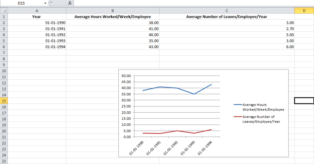
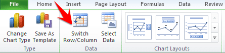
Sometimes if you do not assign the right data type to your columns in the first step, the graph may not show in a way that you want it to. For example, Excel may plot the parameter Average Number of Leaves/Employee/Year along the X axis instead of the Year. In this case, you can use the option Switch Row/Column under the Design tab of Chart Tools to play around with various combinations of X axis and Y axis parameters till you hit on the perfect rendition.

To change colors or to change the design of your graph, go to Chart Tools in the Excel header.

You can select from the design, layout and format. Each will change up the look and feel of your Excel graph.

Design: Design allows you to move your graph and re-position it. It gives you the freedom to change the chart type. You can even experiment with different chart layouts. This may conform more to your brand guidelines, your personal style, or your manager’s preference.

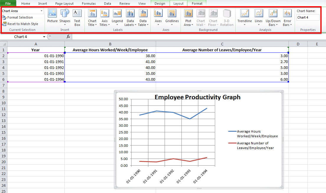
Layout: This allows you to change the title of the axis, the title of your chart and the position of the legend. You might go with vertical text along the Y axis and horizontal text along the X axis. You can even adjust the grid lines. You have every formatting tool conceivable at your fingertips to improve the look and feel of your graph.

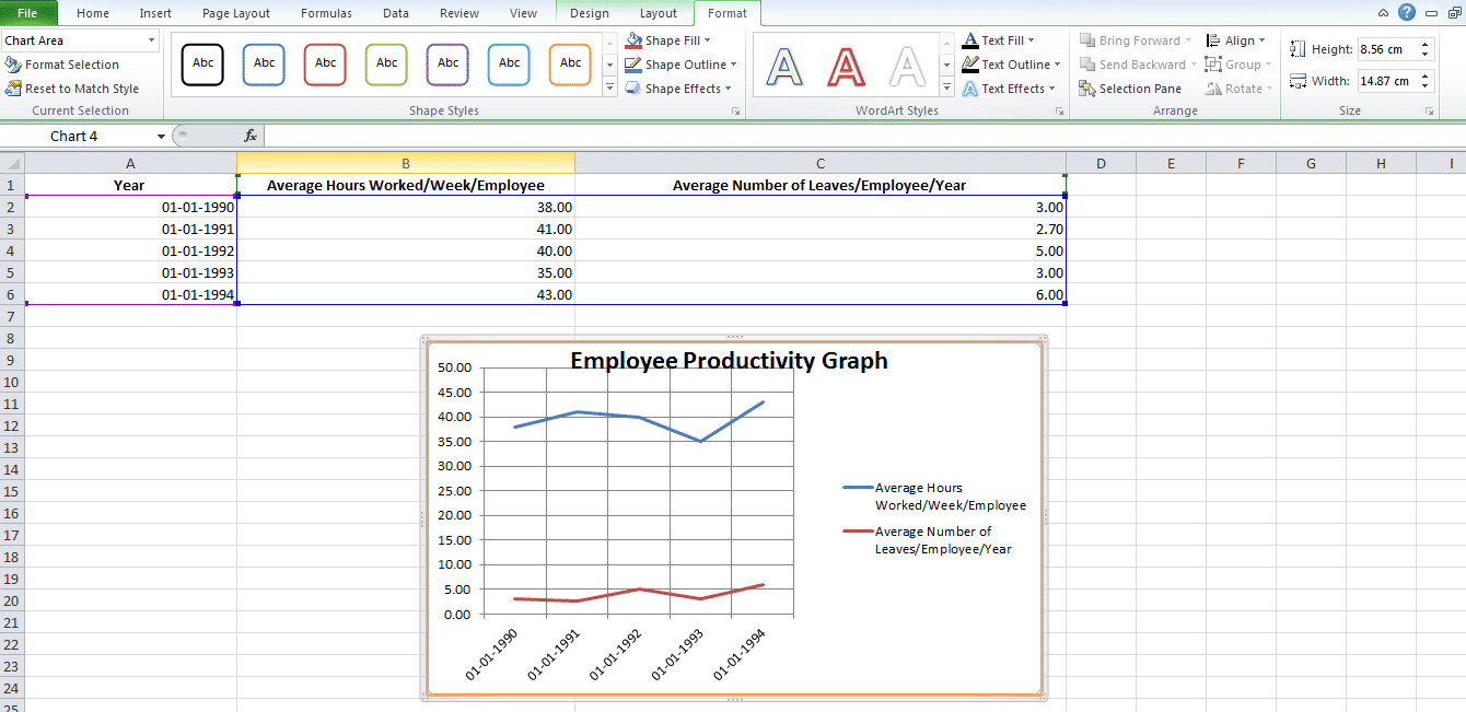
Format: The Format tab allows you to add a border in your chosen width and color around the graph to properly separate it from the data points that are filled in the rows and columns.

And there you have it. An accurate visual representation of the data that you have imported or entered manually to help your team members and stakeholders better engage with the information and utilize it to create strategies or be more aware of all the constraints while taking decisions!

Challenges with Making a Graph In Excel

When manipulating simple data sets, you can create a graph fairly easily.

But when you start adding in several types of data with multiple parameters, then there will be glitches. Here are some of the challenges that you’re going to have:

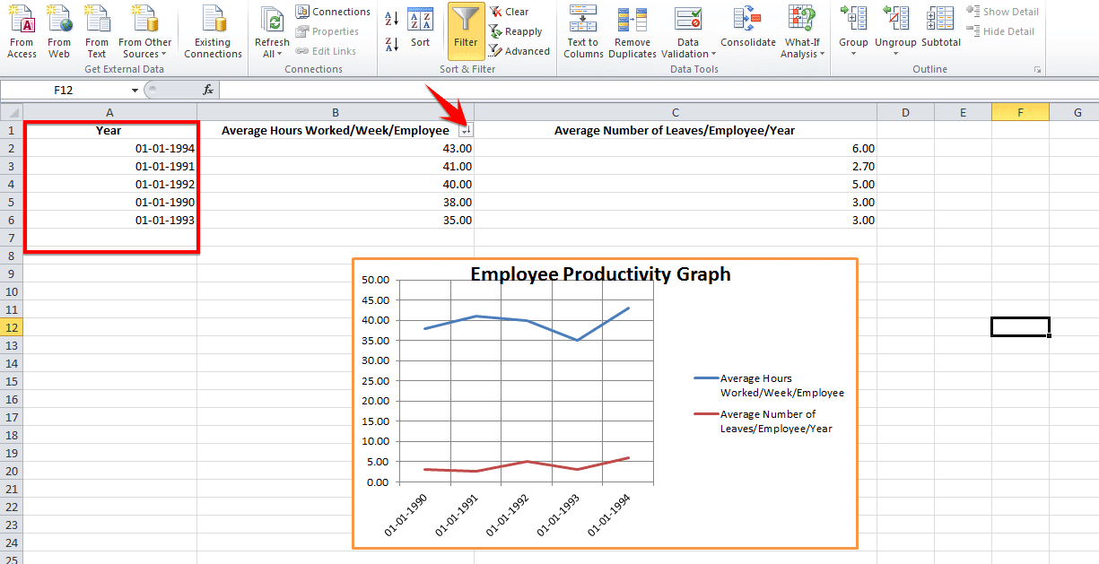
• Data sorting can be problematic when creating graphs. Online tutorials might recommend data sorting to make your “charts” look more aesthetically appealing. But beware of when the X axis is a time-based parameter! Sorting data values by magnitude may mess up the flow of the graph because the dates are sorted randomly. You may not be able to spot the trends very well.

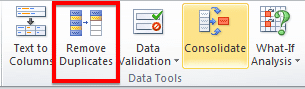
You may forget to remove duplicates. This is especially true if you have imported the data from a third-party application. Generally, this type of information is not filtered of redundancies. And you might end up corrupting the integrity of your information if duplicates sneak into your pictorial representation of trends. When working with copious volumes of data, it is best to use the Remove Duplicates option on your rows.

Creating graphs in Excel doesn’t have to be overly complex, but, much like with creating Gantt charts in Excel, there can be some easier tools to help you do it. If you’re trying to create graphs for workloads, budget allocations or monitoring projects, check out project management software instead.

Many of those functions are automated and without manual data entry. And you won’t be left wondering about who has the latest data sets. Most project management solutions, like Workzone, have file sharing and some visualization capabilities built-in.

Источник

---

Often you may be interested in plotting an equation or a function in Excel. Fortunately this is easy to do with built-in Excel formulas.

This tutorial provides several examples of how to plot equations/functions in Excel.

Example 1: Plot a Linear Equation

Suppose you’d like to plot the following equation:

y = 2x + 5

The following image shows how to create the y-values for this linear equation in Excel, using the range of 1 to 10 for the x-values:

Next, highlight the values in the range A2:B11. Then click on the Insert tab. Within the Charts group, click on the plot option called Scatter.

The following plot will automatically appear:

We can see that the plot follows a straight line since the equation that we used was linear in nature.

Example 2: Plot a Quadratic Equation

Suppose you’d like to plot the following equation:

y = 3x²

The following image shows how to create the y-values for this equation in Excel, using the range of 1 to 10 for the x-values:

Next, highlight the values in the range A2:B11. Then click on the Insert tab. Within the Charts group, click on the plot option called Scatter.

The following plot will automatically appear:

We can see that the plot follows a curved line since the equation that we used was quadratic.

Example 3: Plot a Reciprocal Equation

Suppose you’d like to plot the following equation:

y = 1/x

The following image shows how to create the y-values for this equation in Excel, using the range of 1 to 10 for the x-values:

Next, highlight the values in the range A2:B11. Then click on the Insert tab. Within the Charts group, click on the plot option called Scatter.

The following plot will automatically appear:

We can see that the plot follows a curved line downwards since this represents the equation y = 1/x.

Example 4: Plot a Sine Equation

Suppose you’d like to plot the following equation:

y = sin(x)

The following image shows how to create the y-values for this equation in Excel, using the range of 1 to 10 for the x-values:

Next, highlight the values in the range A2:B11. Then click on the Insert tab. Within the Charts group, click on the plot option called Scatter with Smooth Lines and Markers.

The following plot will automatically appear:

Conclusion

You can use a similar technique to plot any function or equation in Excel. Simply choose a range of x-values to use in one column, then use an equation in a separate column to define the y-values based on the x-values.