Equal to this or that excel

Using IF with AND, OR and NOT functions

The IF function allows you to make a logical comparison between a value and what you expect by testing for a condition and returning a result if that condition is True or False.

=IF(Something is True, then do something, otherwise do something else)

But what if you need to test multiple conditions, where let’s say all conditions need to be True or False ( AND), or only one condition needs to be True or False ( OR), or if you want to check if a condition does NOT meet your criteria? All 3 functions can be used on their own, but it’s much more common to see them paired with IF functions.

Use the IF function along with AND, OR and NOT to perform multiple evaluations if conditions are True or False.

IF(AND()) — IF(AND(logical1, [logical2], . ), value_if_true, [value_if_false]))

IF(OR()) — IF(OR(logical1, [logical2], . ), value_if_true, [value_if_false]))

IF(NOT()) — IF(NOT(logical1), value_if_true, [value_if_false]))

The condition you want to test.

The value that you want returned if the result of logical_test is TRUE.

The value that you want returned if the result of logical_test is FALSE.

Here are overviews of how to structure AND, OR and NOT functions individually. When you combine each one of them with an IF statement, they read like this:

AND – =IF(AND(Something is True, Something else is True), Value if True, Value if False)

OR – =IF(OR(Something is True, Something else is True), Value if True, Value if False)

NOT – =IF(NOT(Something is True), Value if True, Value if False)

Examples

Following are examples of some common nested IF(AND()), IF(OR()) and IF(NOT()) statements. The AND and OR functions can support up to 255 individual conditions, but it’s not good practice to use more than a few because complex, nested formulas can get very difficult to build, test and maintain. The NOT function only takes one condition.

Here are the formulas spelled out according to their logic:

=IF(AND(A2>0,B2 0,B4 50),TRUE,FALSE)

IF A6 (25) is NOT greater than 50, then return TRUE, otherwise return FALSE. In this case 25 is not greater than 50, so the formula returns TRUE.

IF A7 (“Blue”) is NOT equal to “Red”, then return TRUE, otherwise return FALSE.

Note that all of the examples have a closing parenthesis after their respective conditions are entered. The remaining True/False arguments are then left as part of the outer IF statement. You can also substitute Text or Numeric values for the TRUE/FALSE values to be returned in the examples.

Here are some examples of using AND, OR and NOT to evaluate dates.

Here are the formulas spelled out according to their logic:

IF A2 is greater than B2, return TRUE, otherwise return FALSE. 03/12/14 is greater than 01/01/14, so the formula returns TRUE.

=IF(AND(A3>B2,A3 B2,A4 B2),TRUE,FALSE)

IF A5 is not greater than B2, then return TRUE, otherwise return FALSE. In this case, A5 is greater than B2, so the formula returns FALSE.

Using AND, OR and NOT with Conditional Formatting

You can also use AND, OR and NOT to set Conditional Formatting criteria with the formula option. When you do this you can omit the IF function and use AND, OR and NOT on their own.

From the Home tab, click Conditional Formatting > New Rule. Next, select the “ Use a formula to determine which cells to format” option, enter your formula and apply the format of your choice.

Edit Rule dialog showing the Formula method» loading=»lazy»>

Using the earlier Dates example, here is what the formulas would be.

If A2 is greater than B2, format the cell, otherwise do nothing.

=AND(A3>B2,A3 B2,A4 B2)

If A5 is NOT greater than B2, format the cell, otherwise do nothing. In this case A5 is greater than B2, so the result will return FALSE. If you were to change the formula to =NOT(B2>A5) it would return TRUE and the cell would be formatted.

Note: A common error is to enter your formula into Conditional Formatting without the equals sign (=). If you do this you’ll see that the Conditional Formatting dialog will add the equals sign and quotes to the formula — =»OR(A4>B2,A4

Need more help?

​​​​​​​

See also

You can always ask an expert in the Excel Tech Community or get support in the Answers community.

Источник

If NOT this or that

Summary

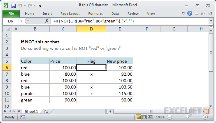
To do something when a cell is NOT this or that (i.e. a cell is NOT equal to «x», «y», etc.) you can use the IF function together with the OR function to run a test. In cell D6, the formula is:

which returns «x» when B6 contains anything except «red» or «green», and an empty string («») otherwise. Notice the OR function is not case-sensitive.

Generic formula

Explanation

The behavior of the IF function can be easily extended by adding logical functions like AND, and OR, to the logical test. If you want to reverse existing logic, you can use the NOT function.

In the example shown, we want to «flag» records where the color is NOT red OR green. In other words, we want to check the colors in column B, and take a specific action if the color is any value other than «red» or «green». In D6, the formula were using is this:

In this formula, the logical test is this bit:

Working from the inside out, we first use the OR function to test for «red» or «green»:

OR will return TRUE if B6 is «red» or «green», and FALSE if B6 contains any other value.

The NOT function simply reverses this result. Adding NOT means the test will return TRUE if B6 is NOT «red» or «green», and FALSE otherwise.

Since we want to flag items that pass our test, we need to take an action when the result of the test is TRUE. In this case, we do that by adding an «x» to column D. If the test is FALSE, we simply add an empty string («»). This causes an «x» to appear in column D when the value in column B is either «red» or «green» and nothing to appear if not.*

You can extend the OR function to check additional conditions as needed.

*If we didn’t add the empty string when FALSE, the formula would actually display FALSE whenever the color is not red.

Increase price if color NOT red or green

You can extend the formula to perform a calculation instead of just returning a fixed value.

For example, say you want to increase all colors except red and green by 15%. In that case, you could use this formula in column E to calculate a new price:

The test is the same as before, the action to take if TRUE is new.

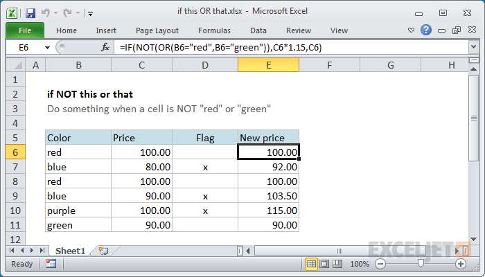
If the result is TRUE, we multiply the original price by 1.15 (to increase by 15%). If the result of the test is FALSE, we simply output the original price.

Источник

“Greater Than or Equal to” (>=) in Excel

The “Greater Than or Equal To” (>=) in Excel

The “greater than or equal to” is a comparison or logical operator that helps compare two data cells of the same data type. It is denoted by the symbol “>=” and returns the following values:

• “True,” if the first value is either greater than or equal to the second value
• “False,” if the first value is smaller than the second value

Generally, the “greater than or equal to” operator is used for date and time values and numbers. It can also be used for textual data.

For example, if cell C1 contains “rose” and cell D1 contains “lotus,” the formula “=C1>=D1” returns “true.” This is because the first letter “r” is greater than the letter “l.” The values “a” and “z” are considered the lowest and the highest text values respectively.

Table of contents

Logical and Arithmetic Operators

The logical operators help draw relevant conclusions which are used in the decision-making process.

The arithmetic operators like “plus” (+), “minus” (-), “asterisk” (*), “forward slash” (/), “percent” (%), and “caret” (^) symbols are used in formulas. These operators are used in calculations to generate numeric output.

The “asterisk,” “forward slash,” and “caret” are used for multiplication, division, and exponentiation respectively.

How to Use “Greater Than” (>) and “Greater Than or Equal to” (>=)?

Let us consider a few examples to understand the usage of the given comparison operators in Excel.

Example #1–“Greater Than” and “Greater Than or Equal to”

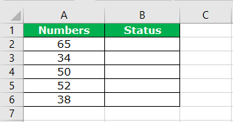
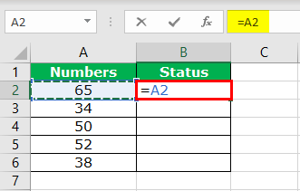
The following list shows five numerical values from cell A2 to A6. We want to test whether each number is greater than 50 or not.

The steps to test the greater number are listed as follows:

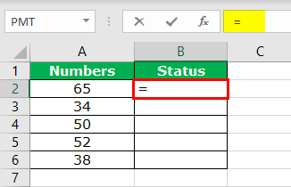
Type the “equal to” (=) sign in cell B2.

Select the cell A2 that is to be tested.

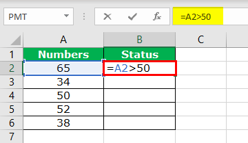
Since we want to test whether the value in cell A2 is greater than 50 or not, type the comparison operator (>) followed by the number 50.

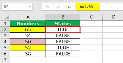
Press the “Enter” key to obtain the result. Copy and paste or drag the formula to the remaining cells. The cells in yellow contain a number greater than 50. Hence, the result is “true”.

The value of cell A4 (50) is not greater than the number 50. Hence, the result in cell B4 is “false”.

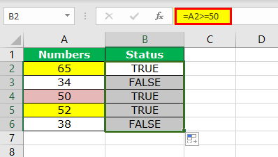
To include 50 in the test, we need to change the comparison operator to “greater than or equal to” (>=).

The “greater than or equal to” operator returns the value “true” in cell B4. This implies that the value of cell A4 is either greater than or equal to 50.

Example #2–“Greater Than or Equal to” With the IF Function

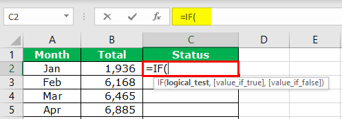
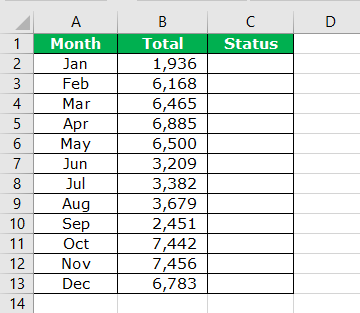
The following table shows the total sales (in dollars) of various months. The monthly incentives are calculated by comparing the sales against the benchmark of $6500. The possibilities are stated as follows:

• If the total sales>$6500, incentives are calculated at 10%.
• If the total sales

Step 1: Open the IF function. The IF function helps evaluate a criterion and returns “true” or “false” depending on whether the condition is met or not.

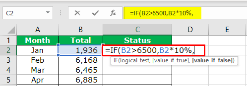
Step 3: The condition is that if the logical test is “true,” we calculate the incentives as B2*10%. So, we type this criterion.

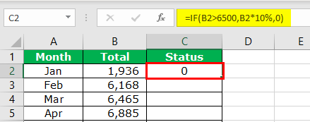
Step 4: If the logical test is “false,” the incentives are 0. So, we type zero at the end of the formula.

In cell C2, the formula returns the output 0. This implies that the value in cell B2 is less than $6500.

Step 5: Drag the formula to the remaining cells, as shown in the following image.

Since the values in the cells B5, B11, B12, and B13 are greater than $6500, we get the respective incentive amounts in column C.

Example #3–“Greater Than or Equal to” With the COUNTIF Function

The following table shows the date and amount of the invoices sent to the buyer. We want to count the number of invoices that are sent on or after 14 th March 2019.

Step 1: Open the COUNTIF function. The COUNTIF function helps count the cells within a particular range based on a criterion.

Step 2: Select the date column (column A) as the range (A2:A13).

Step 3: Since the criterion is on or after 14 th March 2019, it can be represented as “>=14-03-2019.” Type the symbol “>=” in double quotation marks.

Note: The comparison operators in the “criteria” argument must be placed within double quotation marks.

Step 5: Close the brackets of the formula and press the “Enter” key.

The output is 7, implying that a total of seven invoices are generated on or after 14 th March 2019.

Example #4–“Greater Than or Equal to” With the SUMIF Function

The following table shows the monthly sales of an organization. The sales figures are reported in thousand dollars. We want to find whether the total sales are greater than or equal to $20,000.

Step 1: Open the SUMIF function. The SUMIF function sums the cells based on a specified criterion.

Step 2: Select the sales column (column B) as the “range” ($B$2:$B$13). This helps sum the monthly sales values.

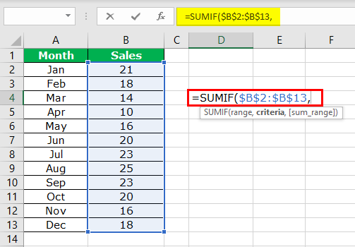
Step 3: Type the “criteria” as “>=”&20. Place the comparison operator within the double quotation marks.

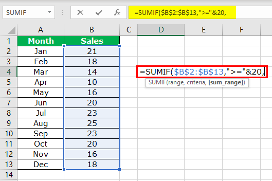
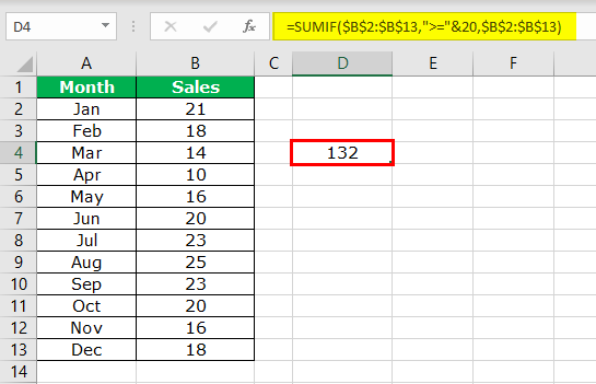
Step 4: Select the “sum_range” same as the “range” argument, i.e., $B$2:$B$13.

The output is $132,000. Hence the total sales are greater than $20,000.

Frequently Asked Questions

The “greater than or equal to” (>=) is one of the six comparison or logical operators of Excel. It returns “true” if the first number is greater than or equal to the second number; otherwise returns “false”.

The remaining comparison operators are “equal to” (=), “not equal to” (<>), “greater than” (>), “less than” ( =SUM(F2:H11)” returns “true” if the value in cell C2 is greater than or equal to the sum of values in the range F2:H11. If the converse is correct, it returns “false”.

The given comparison operator should be used in the following situations:

• To find which of the two quantities is greater or smaller
• To find whether one quantity is equal to the other
• To evaluate two quantities with respect to a given criteria
• To compare two separate quantities with a third quantity

Note: Two quantities can be compared only if both are of the same data type.

The “greater than or equal to” symbol (>=) is written in Excel by typing the “greater than” (>) sign followed by the “equal to” (=) operator.

The operator “>=” is placed between two numbers or cell references to be compared. For example, type the formula as “=A1>=A2” in Excel.

The symbol “>=” is placed within double quotation marks when entered in the “criteria” argument of SUMIF and COUNTIF functions. For example, type the formula as “=SUMIF(B2:B11,”>=100″)” in Excel.

Note: The two formulas of Excel (in the preceding examples) should be entered excluding spaces and without the beginning and ending quotation marks.

Recommended Articles

This has been a guide to “greater than or equal to” in Excel. Here we discuss how to use “greater than” and “greater than or equal to” (>=) with IF, SUMIF, and COUNTIF formulas along with examples and downloadable Excel templates. You may also look at these useful functions in Excel –

Источник

The “greater than or equal to” is a comparison or logical operator that helps compare two data cells of the same data type. It is denoted by the symbol “>=” and returns the following values:

• “True,” if the first value is either greater than or equal to the second value
• “False,” if the first value is smaller than the second value

Generally, the “greater than or equal to” operator is used for date and time values and numbers. It can also be used for textual data.

For example, if cell C1 contains “rose” and cell D1 contains “lotus,” the formula “=C1>=D1” returns “true.” This is because the first letter “r” is greater than the letter “l.” The values “a” and “z” are considered the lowest and the highest text values respectively.

Logical and Arithmetic Operators

The “equal to” (=) symbol, used in mathematical operations, helps find whether two values are equal or not. Likewise, every logical operatorLogical operators in excel are also known as the comparison operators and they are used to compare two or more values, the return output given by these operators are either true or false, we get true value when the conditions match the criteria and false as a result when the conditions do not match the criteria.read more serves a particular purpose. Since logical operators return only the Boolean values “true” or “false,” they are also called Boolean operators.

The logical operators help draw relevant conclusions which are used in the decision-making process.

 The arithmetic operators like “plus” (+), “minus” (-), “asterisk” (*), “forward slash” (/), “percent” (%), and “caret” (^) symbols are used in formulas. These operators are used in calculations to generate numeric output.

The “asterisk,” “forward slash,” and “caret” are used for multiplication, division, and exponentiation respectively.

How to Use “Greater Than” (>) and “Greater Than or Equal to” (>=)?

Let us consider a few examples to understand the usage of the given comparison operators in Excel.

You can download this Greater Than or Equal to Excel Template here – Greater Than or Equal to Excel Template

Example #1–“Greater Than” and “Greater Than or Equal to”

The following list shows five numerical values from cell A2 to A6. We want to test whether each number is greater than 50 or not.

Example #2–“Greater Than or Equal to” With the IF Function

Let us use the comparison operator “greater than or equal to” with the IF conditionIF function in Excel evaluates whether a given condition is met and returns a value depending on whether the result is “true” or “false”. It is a conditional function of Excel, which returns the result based on the fulfillment or non-fulfillment of the given criteria.
read more.

The following table shows the total sales (in dollars) of various months. The monthly incentives are calculated by comparing the sales against the benchmark of $6500. The possibilities are stated as follows:

• If the total sales>$6500, incentives are calculated at 10%.
• If the total sales<$6500, incentives are 0.

Step 1: Open the IF function. The IF function helps evaluate a criterion and returns “true” or “false” depending on whether the condition is met or not.

Step 2: Apply the logical testA logical test in Excel results in an analytical output, either true or false. The equals to operator, “=,” is the most commonly used logical test.read more, B2>6500.

Step 3: The condition is that if the logical test is “true,” we calculate the incentives as B2*10%. So, we type this criterion.

Step 4: If the logical test is “false,” the incentives are 0. So, we type zero at the end of the formula.

In cell C2, the formula returns the output 0. This implies that the value in cell B2 is less than $6500.

Step 5: Drag the formula to the remaining cells, as shown in the following image.

Since the values in the cells B5, B11, B12, and B13 are greater than $6500, we get the respective incentive amounts in column C.

Example #3–“Greater Than or Equal to” With the COUNTIF Function

Let us use the comparison operator “greater than or equal to” with the COUNTIFThe COUNTIF function in Excel counts the number of cells within a range based on pre-defined criteria. It is used to count cells that include dates, numbers, or text. For example, COUNTIF(A1:A10,”Trump”) will count the number of cells within the range A1:A10 that contain the text “Trump”
read more function.

The following table shows the date and amount of the invoices sent to the buyer. We want to count the number of invoices that are sent on or after 14^th March 2019.

Step 1: Open the COUNTIF function. The COUNTIF function helps count the cells within a particular range based on a criterion.

Step 2: Select the date column (column A) as the range (A2:A13).

Step 3: Since the criterion is on or after 14^th March 2019, it can be represented as “>=14-03-2019.” Type the symbol “>=” in double quotation marks.

Note: The comparison operators in the “criteria” argument must be placed within double quotation marks.

Step 4: Type the ampersand sign (&). We supply the date with the DATE functionThe date function in excel is a date and time function representing the number provided as arguments in a date and time code. The result displayed is in date format, but the arguments are supplied as integers.read more. This is because we are not using the cell referencesCell reference in excel is referring the other cells to a cell to use its values or properties. For instance, if we have data in cell A2 and want to use that in cell A1, use =A2 in cell A1, and this will copy the A2 value in A1.read more of date values.

Step 5: Close the brackets of the formula and press the “Enter” key.

The output is 7, implying that a total of seven invoices are generated on or after 14^th March 2019.

Example #4–“Greater Than or Equal to” With the SUMIF Function

Let us use the comparison operator “greater than or equal to” with the SUMIFThe SUMIF Excel function calculates the sum of a range of cells based on given criteria. The criteria can include dates, numbers, and text. For example, the formula “=SUMIF(B1:B5, “<=12”)” adds the values in the cell range B1:B5, which are less than or equal to 12.
read more function.

The following table shows the monthly sales of an organization. The sales figures are reported in thousand dollars. We want to find whether the total sales are greater than or equal to $20,000.

Step 1: Open the SUMIF function. The SUMIF function sums the cells based on a specified criterion.

Step 2: Select the sales column (column B) as the “range” ($B$2:$B$13). This helps sum the monthly sales values.

Step 3: Type the “criteria” as “>=”&20. Place the comparison operator within the double quotation marks.

Step 4: Select the “sum_range” same as the “range” argument, i.e., $B$2:$B$13.

The output is $132,000. Hence the total sales are greater than $20,000.

Frequently Asked Questions

Recommended Articles

This has been a guide to “greater than or equal to” in Excel. Here we discuss how to use “greater than” and “greater than or equal to” (>=) with IF, SUMIF, and COUNTIF formulas along with examples and downloadable Excel templates. You may also look at these useful functions in Excel –

• “Not Equal” in VBA
• Excel Formula for COUNTIF
• Not Equal to in Excel
• List of Excel Functions