
Logical Operators in Excel: Less Than, Greater Than (+More!)
We all have read about logical operators in high school – even if we didn’t like them then.
Similar to those, Excel provides comparison operators that return the result in TRUE or FALSE.
These operators are like “less than or equal to” and “greater than or equal to” which are very helpful in quick data analysis.
In this guide, we will discuss all the aspects of logical operators and see how to use them. So stay tuned! 🤗
Also, if you want to practice along the guide, you can get our free sample workbook here.
What are logical operators in Excel?
Logical operators are also known as comparison operators because their primary purpose is to compare two values.
These operators always only consider the value. And that’s regardless of how it is derived – even if it’s from a formula.
Also, a logical operator never returns numerical values in the result, only TRUE and FALSE. The value of TRUE and FALSE is 1 and 0, respectively – which are binary digits.
The comparison operators can also handle any Boolean expression. Hence, they are called Boolean operators.
In Excel, there are six Boolean operators you can use. These are:
- Less than
- Less than or equal to
- Greater than
- Greater than or equal to
- Equal to
- Not Equal to
Let’s study all these operators in depth below 🚀
Less than in Excel
As evident from the name, the ‘Less than’ operator checks if the first value is less than the second value or not. If it is, it returns TRUE; otherwise, it returns FALSE, and it is denoted by <.
Let’s understand its concept using an example.
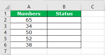
We have the following data set.

We want to check if cell A2 is less than cell B2. For that:
- Select cell C2.
- Type in the formula
=A2<B2

- Press Enter.
Excel shows the result as follows:

To do the same for all other entries, simply double-click the Fill Handle as:

Pro Tip!
Excel can also compare text values, but by their alphabetical order. It compares the first letters of both values. And determines which of the two falls lower in the order.
However, if both the first values are the same, the operator moves on to the second one, and so forth 😀
Less than or equal to in Excel
The ‘Less than or equal to’ operator is the same as the ‘Less than’ operator. The only difference is that it returns TRUE if the first value is smaller or equal to the second value. It is represented by <=
Let’s see it working through a quick example.
We have identical values in the first two cells below.

If we apply the formula:
=A2<=B2
Excel would return the result TRUE.

Similarly, if we reduce the value of cell A2, it would still show TRUE as:

That’s because the condition is to return TRUE if the first value is less than or equal to the second value. Since the value, in this case, is lesser, Excel returns TRUE. Otherwise, it would return FALSE.
Less than or equal to’ example with the IF function
You can also combine logical operators with Excel functions.
Let’s see an example using the IF function with the ‘Less than or equal to’ operator below.
Suppose, we have the following data set.

We want to check if the first value in A2 is less than or equal to the value in cell B2 or not. If it is, the IF function will return ‘Right,’ and if it is not, it will return ‘Wrong.’
So, for this, we will enter the formula:
=IF (A1<=B1, “Right,” “Wrong”)


The IF function returns “Right” because the values in cells A2 and B2 are equal.
Double Click the Fill Handle to copy the formula to the remaining entries.

Excel returns “Right” for all the values that fulfill the condition, i.e., are less than or equal to the second value. And for the ones that don’t fulfill the condition, Excel returns “Wrong.”
Greater than in Excel
The ‘Greater than’ logical operator checks if the first value is greater than the second. It’s the opposite of the ‘Less than’ operator and is denoted by >.
Let’s see it using an example 👀
We have the following data.

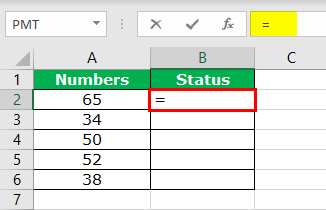
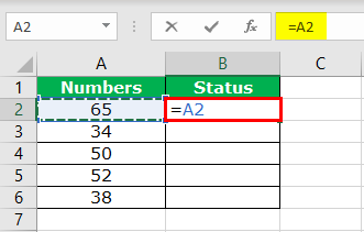
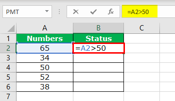
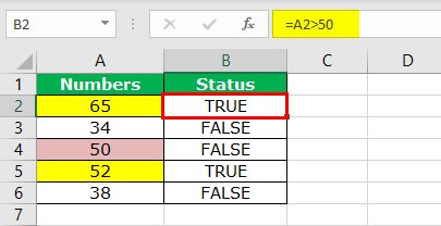
We want to check if the value in cell A2 is greater than the value in cell B2. For that:
- Select C2.
- Enter the formula
=A2>B2

- Hit Enter.

The result TRUE shows that cell A2 is greater than cell B2.
Drag down the Fill Handle to copy the formula.

Pro Tip!
For text values, the ‘Greater than’ operator begins the count from the bottom of the English alphabet – Z.
‘Greater than’ example with the SUMIF Function
Let’s see how to use the ‘Greater than’ operator with the SUMIF function below.
We have the following sample data.

To use the SUMIF function, we will apply the formula:
=SUMIF(A2:A7, “>”&B2, B2:B7)

Note that we have used the “&” ampersand after the logical operator. This is because our target value was in another cell, so we used the cell reference and joined it with the condition.
Comment
Make sure to enclose the logical operators in double quotation marks as we did above. Otherwise, they are considered to be text strings.
Press Enter and Excel returns the result:

And tada! It’s done. That’s how easy it is to use the SUMIF function with the ‘Greater than’ operator 😉
Greater than or equal to in Excel
As the name suggests, the ‘Greater than or equal’ sign tells if a value is greater than or equal to its counterpart. If it is, the operator returns TRUE otherwise, it returns FALSE. The ‘Greater than or equal’ operator is denoted by ≥.
Let’s see how it works through an example below.
We have the following example data.
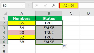
If we apply the ‘Greater than or equal to’ operator on cells A2 and B2 as:
=A2>=B2

Excel returns TRUE as both the values are equal to each other.

Similarly, if we increase the value of cell A2 by 1, the result will remain the same.

That’s because the condition given is to check if the value in the first cell is greater than the value in the second cell or equal to it.
Not equal to in Excel
The ‘Not equal to’ operator is self-explanatory!
But the symbol is not🤔
It is denoted <>, and it returns FALSE if two values are equal to each other; otherwise, it returns TRUE. It is the opposite of the ‘Equal to’ operator.
Let’s see it in action through an example.
This is our sample data.

We will apply the ‘Not equal to’ operator to cells A2 and B2 as:
=A2<>B2

Excel returns FALSE as a result:

Here Excel returned FALSE because both the cell values were the same. And the ‘Not equal to’ operator returns FALSE for identical values.
To copy the same formula down the rows, double-click the Fill Handle.

Excel copied the formula to the remaining rows 😊
That’s it – Now what?
And tada! You now know everything about Excel logical operators 🥳
We learned so much about them in this article. We saw how the ‘Less than’ and ‘Greater than’ operators work. We also learned how to use them with text values and interpret the answer.
All this knowledge takes us one step closer to Excel mastery. But it doesn’t end here. This giant spreadsheet has tons of other things to offer.
If you want to polish your Excel skills, we recommend you master the VLOOKUP, IF, and SUMIF functions.
You learn those in my 30-minute free course delivered straight to your inbox. So enroll now and learn these fantastic functions!
Other resources
Boolean operators are very useful when you need quick results for extensive data. And even more useful when combined with Excel functions like COUNTIF function and SUMIF function, etc.
If you enjoyed reading this article, we bet you’d want to learn more. Some related topics include the IF, TRUE & FALSE, and Excel Logical Functions.
Frequently asked questions
It’s simple. You can use the ‘Less than or equal to’ operator in formulas like =A3<= SUM(C2:C6). Excel will return the result TRUE if the value in A3 is less than or equal to the result of SUM; otherwise FALSE.
Yes, you can. The >= operator symbolizes the ‘Greater than or equal’ condition. It returns TRUE if a certain value is greater than or equal to its counterpart and vice versa.
Excel lets you use logical operators with multiple Excel functions. The IF function is most common for combining with comparison operators. An example could be =IF (A1>=B1, “Pass,” “Fail”). This tells the function to return Pass if the condition is TRUE; otherwise, Fail.
Kasper Langmann2023-01-04T18:52:07+00:00
Page load link
The “greater than or equal to” is a comparison or logical operator that helps compare two data cells of the same data type. It is denoted by the symbol “>=” and returns the following values:
- “True,” if the first value is either greater than or equal to the second value
- “False,” if the first value is smaller than the second value
Generally, the “greater than or equal to” operator is used for date and time values and numbers. It can also be used for textual data.
For example, if cell C1 contains “rose” and cell D1 contains “lotus,” the formula “=C1>=D1” returns “true.” This is because the first letter “r” is greater than the letter “l.” The values “a” and “z” are considered the lowest and the highest text values respectively.
Table of contents
- The “Greater Than or Equal To” (>=) in Excel
- Logical and Arithmetic Operators
- How to Use “Greater Than” (>) and “Greater Than or Equal to” (>=)?
- Example #1–“Greater Than” and “Greater Than or Equal to”
- Example #2–“Greater Than or Equal to” With the IF Function
- Example #3–“Greater Than or Equal to” With the COUNTIF Function
- Example #4–“Greater Than or Equal to” With the SUMIF Function
- Frequently Asked Questions
- Recommended Articles
Logical and Arithmetic Operators
The “equal to” (=) symbol, used in mathematical operations, helps find whether two values are equal or not. Likewise, every logical operatorLogical operators in excel are also known as the comparison operators and they are used to compare two or more values, the return output given by these operators are either true or false, we get true value when the conditions match the criteria and false as a result when the conditions do not match the criteria.read more serves a particular purpose. Since logical operators return only the Boolean values “true” or “false,” they are also called Boolean operators.
The logical operators help draw relevant conclusions which are used in the decision-making process.
The arithmetic operators like “plus” (+), “minus” (-), “asterisk” (*), “forward slash” (/), “percent” (%), and “caret” (^) symbols are used in formulas. These operators are used in calculations to generate numeric output.
The “asterisk,” “forward slash,” and “caret” are used for multiplication, division, and exponentiation respectively.
How to Use “Greater Than” (>) and “Greater Than or Equal to” (>=)?
Let us consider a few examples to understand the usage of the given comparison operators in Excel.
You can download this Greater Than or Equal to Excel Template here – Greater Than or Equal to Excel Template
Example #1–“Greater Than” and “Greater Than or Equal to”
The following list shows five numerical values from cell A2 to A6. We want to test whether each number is greater than 50 or not.
The steps to test the greater number are listed as follows:
- Type the “equal to” (=) sign in cell B2.

- Select the cell A2 that is to be tested.

- Since we want to test whether the value in cell A2 is greater than 50 or not, type the comparison operator (>) followed by the number 50.

- Press the “Enter” key to obtain the result. Copy and paste or drag the formula to the remaining cells. The cells in yellow contain a number greater than 50. Hence, the result is “true”.
The value of cell A4 (50) is not greater than the number 50. Hence, the result in cell B4 is “false”.

To include 50 in the test, we need to change the comparison operator to “greater than or equal to” (>=).
The “greater than or equal to” operator returns the value “true” in cell B4. This implies that the value of cell A4 is either greater than or equal to 50.

Example #2–“Greater Than or Equal to” With the IF Function
Let us use the comparison operator “greater than or equal to” with the IF conditionIF function in Excel evaluates whether a given condition is met and returns a value depending on whether the result is “true” or “false”. It is a conditional function of Excel, which returns the result based on the fulfillment or non-fulfillment of the given criteria.
read more.
The following table shows the total sales (in dollars) of various months. The monthly incentives are calculated by comparing the sales against the benchmark of $6500. The possibilities are stated as follows:
- If the total sales>$6500, incentives are calculated at 10%.
- If the total sales<$6500, incentives are 0.
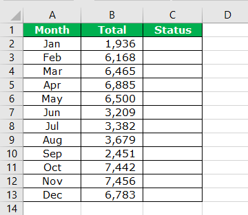
Step 1: Open the IF function. The IF function helps evaluate a criterion and returns “true” or “false” depending on whether the condition is met or not.
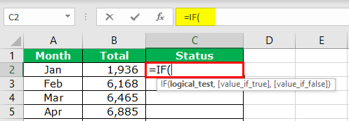
Step 2: Apply the logical testA logical test in Excel results in an analytical output, either true or false. The equals to operator, “=,” is the most commonly used logical test.read more, B2>6500.

Step 3: The condition is that if the logical test is “true,” we calculate the incentives as B2*10%. So, we type this criterion.
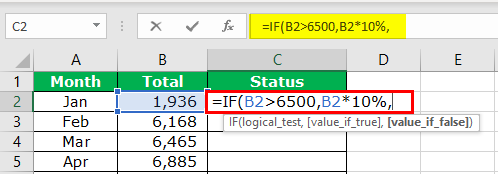
Step 4: If the logical test is “false,” the incentives are 0. So, we type zero at the end of the formula.
In cell C2, the formula returns the output 0. This implies that the value in cell B2 is less than $6500.
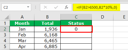
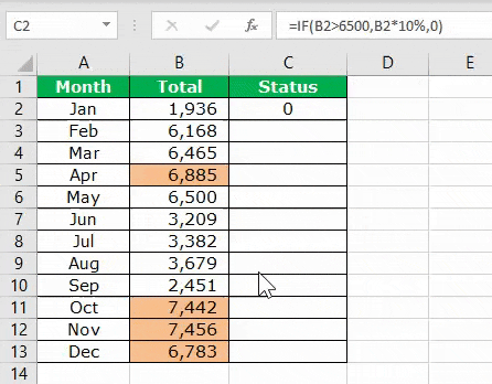
Step 5: Drag the formula to the remaining cells, as shown in the following image.
Since the values in the cells B5, B11, B12, and B13 are greater than $6500, we get the respective incentive amounts in column C.
Example #3–“Greater Than or Equal to” With the COUNTIF Function
Let us use the comparison operator “greater than or equal to” with the COUNTIFThe COUNTIF function in Excel counts the number of cells within a range based on pre-defined criteria. It is used to count cells that include dates, numbers, or text. For example, COUNTIF(A1:A10,”Trump”) will count the number of cells within the range A1:A10 that contain the text “Trump”
read more function.
The following table shows the date and amount of the invoices sent to the buyer. We want to count the number of invoices that are sent on or after 14th March 2019.

Step 1: Open the COUNTIF function. The COUNTIF function helps count the cells within a particular range based on a criterion.

Step 2: Select the date column (column A) as the range (A2:A13).

Step 3: Since the criterion is on or after 14th March 2019, it can be represented as “>=14-03-2019.” Type the symbol “>=” in double quotation marks.
Note: The comparison operators in the “criteria” argument must be placed within double quotation marks.

Step 4: Type the ampersand sign (&). We supply the date with the DATE functionThe date function in excel is a date and time function representing the number provided as arguments in a date and time code. The result displayed is in date format, but the arguments are supplied as integers.read more. This is because we are not using the cell referencesCell reference in excel is referring the other cells to a cell to use its values or properties. For instance, if we have data in cell A2 and want to use that in cell A1, use =A2 in cell A1, and this will copy the A2 value in A1.read more of date values.

Step 5: Close the brackets of the formula and press the “Enter” key.
The output is 7, implying that a total of seven invoices are generated on or after 14th March 2019.

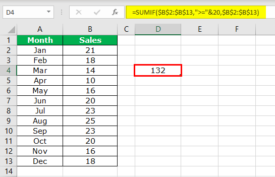
Example #4–“Greater Than or Equal to” With the SUMIF Function
Let us use the comparison operator “greater than or equal to” with the SUMIFThe SUMIF Excel function calculates the sum of a range of cells based on given criteria. The criteria can include dates, numbers, and text. For example, the formula “=SUMIF(B1:B5, “<=12”)” adds the values in the cell range B1:B5, which are less than or equal to 12.
read more function.
The following table shows the monthly sales of an organization. The sales figures are reported in thousand dollars. We want to find whether the total sales are greater than or equal to $20,000.

Step 1: Open the SUMIF function. The SUMIF function sums the cells based on a specified criterion.

Step 2: Select the sales column (column B) as the “range” ($B$2:$B$13). This helps sum the monthly sales values.
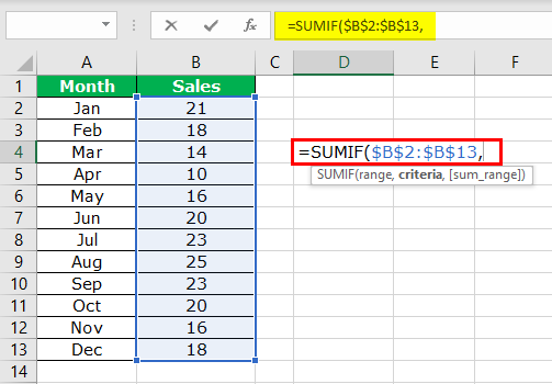
Step 3: Type the “criteria” as “>=”&20. Place the comparison operator within the double quotation marks.
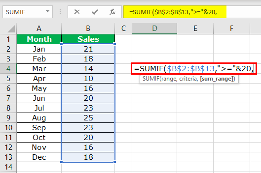
Step 4: Select the “sum_range” same as the “range” argument, i.e., $B$2:$B$13.
The output is $132,000. Hence the total sales are greater than $20,000.
Frequently Asked Questions
Define the “greater than or equal to” operator in Excel.
The “greater than or equal to” (>=) is one of the six comparison or logical operators of Excel. It returns “true” if the first number is greater than or equal to the second number; otherwise returns “false”.
The remaining comparison operators are “equal to” (=), “not equal to” (<>), “greater than” (>), “less than” (<), and “less than or equal to” (<=). All the comparison operators help compare two data cells. They can be used with numbers, text, and date and time values.
For example, the formula “=C2>=SUM(F2:H11)” returns “true” if the value in cell C2 is greater than or equal to the sum of values in the range F2:H11. If the converse is correct, it returns “false”.
When should the “greater than or equal to” operator be used in Excel?
The given comparison operator should be used in the following situations:
• To find which of the two quantities is greater or smaller
• To find whether one quantity is equal to the other
• To evaluate two quantities with respect to a given criteria
• To compare two separate quantities with a third quantity
Note: Two quantities can be compared only if both are of the same data type.
How is the “greater than or equal to” symbol written in Excel?
The “greater than or equal to” symbol (>=) is written in Excel by typing the “greater than” (>) sign followed by the “equal to” (=) operator.
The operator “>=” is placed between two numbers or cell references to be compared. For example, type the formula as “=A1>=A2” in Excel.
The symbol “>=” is placed within double quotation marks when entered in the “criteria” argument of SUMIF and COUNTIF functions. For example, type the formula as “=SUMIF(B2:B11,”>=100″)” in Excel.
Note: The two formulas of Excel (in the preceding examples) should be entered excluding spaces and without the beginning and ending quotation marks.
Recommended Articles
This has been a guide to “greater than or equal to” in Excel. Here we discuss how to use “greater than” and “greater than or equal to” (>=) with IF, SUMIF, and COUNTIF formulas along with examples and downloadable Excel templates. You may also look at these useful functions in Excel –
- “Not Equal” in VBA
- Excel Formula for COUNTIF
- Not Equal to in Excel
- List of Excel Functions
Содержание
- Using IF with AND, OR and NOT functions
- Examples
- Using AND, OR and NOT with Conditional Formatting
- Need more help?
- See also
- Comparison Operators
- Equal to
- Greater than
- Less than
- Greater than or equal to
- Less than or equal to
- Excel: check if two cells match or multiple cells are equal
- How to check if two cells match in Excel
- If two cells equal, return TRUE
- If two cells match, return value
- If one cell equals another, then return another cell
- Case-sensitive formula to see if two cells match
- How to check if multiple cells are equal
- AND formula to see if multiple cells match
- COUNTIF formula to check if multiple columns match
- Case-sensitive formula for multiple matches
- Check if cell matches any cell in range
- Check if two ranges are equal
Using IF with AND, OR and NOT functions
The IF function allows you to make a logical comparison between a value and what you expect by testing for a condition and returning a result if that condition is True or False.
=IF(Something is True, then do something, otherwise do something else)
But what if you need to test multiple conditions, where let’s say all conditions need to be True or False ( AND), or only one condition needs to be True or False ( OR), or if you want to check if a condition does NOT meet your criteria? All 3 functions can be used on their own, but it’s much more common to see them paired with IF functions.
Use the IF function along with AND, OR and NOT to perform multiple evaluations if conditions are True or False.
IF(AND()) — IF(AND(logical1, [logical2], . ), value_if_true, [value_if_false]))
IF(OR()) — IF(OR(logical1, [logical2], . ), value_if_true, [value_if_false]))
IF(NOT()) — IF(NOT(logical1), value_if_true, [value_if_false]))
The condition you want to test.
The value that you want returned if the result of logical_test is TRUE.
The value that you want returned if the result of logical_test is FALSE.
Here are overviews of how to structure AND, OR and NOT functions individually. When you combine each one of them with an IF statement, they read like this:
AND – =IF(AND(Something is True, Something else is True), Value if True, Value if False)
OR – =IF(OR(Something is True, Something else is True), Value if True, Value if False)
NOT – =IF(NOT(Something is True), Value if True, Value if False)
Examples
Following are examples of some common nested IF(AND()), IF(OR()) and IF(NOT()) statements. The AND and OR functions can support up to 255 individual conditions, but it’s not good practice to use more than a few because complex, nested formulas can get very difficult to build, test and maintain. The NOT function only takes one condition.

Here are the formulas spelled out according to their logic:
=IF(AND(A2>0,B2 0,B4 50),TRUE,FALSE)
IF A6 (25) is NOT greater than 50, then return TRUE, otherwise return FALSE. In this case 25 is not greater than 50, so the formula returns TRUE.
IF A7 (“Blue”) is NOT equal to “Red”, then return TRUE, otherwise return FALSE.
Note that all of the examples have a closing parenthesis after their respective conditions are entered. The remaining True/False arguments are then left as part of the outer IF statement. You can also substitute Text or Numeric values for the TRUE/FALSE values to be returned in the examples.
Here are some examples of using AND, OR and NOT to evaluate dates.

Here are the formulas spelled out according to their logic:
IF A2 is greater than B2, return TRUE, otherwise return FALSE. 03/12/14 is greater than 01/01/14, so the formula returns TRUE.
=IF(AND(A3>B2,A3 B2,A4 B2),TRUE,FALSE)
IF A5 is not greater than B2, then return TRUE, otherwise return FALSE. In this case, A5 is greater than B2, so the formula returns FALSE.

Using AND, OR and NOT with Conditional Formatting
You can also use AND, OR and NOT to set Conditional Formatting criteria with the formula option. When you do this you can omit the IF function and use AND, OR and NOT on their own.
From the Home tab, click Conditional Formatting > New Rule. Next, select the “ Use a formula to determine which cells to format” option, enter your formula and apply the format of your choice.
 Edit Rule dialog showing the Formula method» loading=»lazy»>
Using the earlier Dates example, here is what the formulas would be.

If A2 is greater than B2, format the cell, otherwise do nothing.
=AND(A3>B2,A3 B2,A4 B2)
If A5 is NOT greater than B2, format the cell, otherwise do nothing. In this case A5 is greater than B2, so the result will return FALSE. If you were to change the formula to =NOT(B2>A5) it would return TRUE and the cell would be formatted.
Note: A common error is to enter your formula into Conditional Formatting without the equals sign (=). If you do this you’ll see that the Conditional Formatting dialog will add the equals sign and quotes to the formula — =»OR(A4>B2,A4
Need more help?

See also
You can always ask an expert in the Excel Tech Community or get support in the Answers community.
Источник
Comparison Operators
Use comparison operators in Excel to check if two values are equal to each other, if one value is greater than another value, if one value is less than another value, etc.
Equal to
The equal to operator (=) returns TRUE if two values are equal to each other.
1. For example, take a look at the formula in cell C1 below.
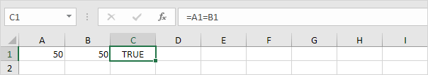
Explanation: the formula returns TRUE because the value in cell A1 is equal to the value in cell B1. Always start a formula with an equal sign (=).
2. The IF function below uses the equal to operator.
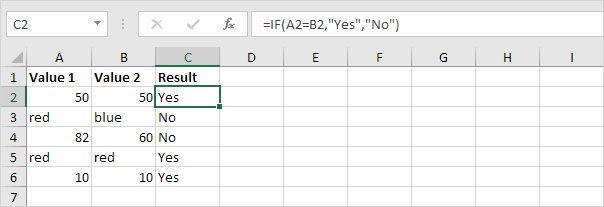
Explanation: if the two values (numbers or text strings) are equal to each other, the IF function returns Yes, else it returns No.
Greater than
The greater than operator (>) returns TRUE if the first value is greater than the second value.
1. For example, take a look at the formula in cell C1 below.
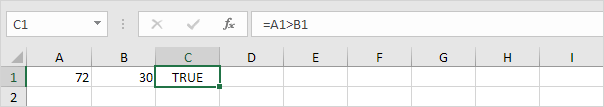
Explanation: the formula returns TRUE because the value in cell A1 is greater than the value in cell B1.
2. The OR function below uses the greater than operator.
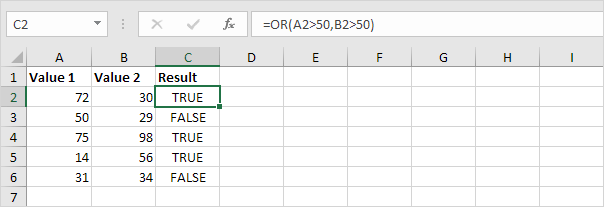
Explanation: this OR function returns TRUE if at least one value is greater than 50, else it returns FALSE.
Less than
The less than operator (
Greater than or equal to
The greater than or equal to operator (>=) returns TRUE if the first value is greater than or equal to the second value.
1. For example, take a look at the formula in cell C1 below.

Explanation: the formula returns TRUE because the value in cell A1 is greater than or equal to the value in cell B1.
2. The COUNTIF function below uses the greater than or equal to operator.
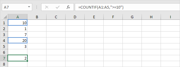
Explanation: this COUNTIF function counts the number of cells that are greater than or equal to 10.
Less than or equal to
The less than or equal to operator ( ) returns TRUE if two values are not equal to each other.
1. For example, take a look at the formula in cell C1 below.
Explanation: the formula returns TRUE because the value in cell A1 is not equal to the value in cell B1.
2. The IF function below uses the not equal to operator.
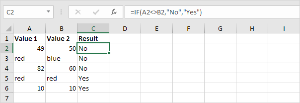
Explanation: if the two values (numbers or text strings) are not equal to each other, the IF function returns No, else it returns Yes.
Источник
Excel: check if two cells match or multiple cells are equal
 by Alexander Frolov, updated on March 13, 2023
The tutorial will teach you how to construct the If match formula in Excel, so it returns logical values, custom text or a value from another cell.
An Excel formula to see if two cells match could be as simple as A1=B1. However, there may be different circumstances when this obvious solution won’t work or produce results different from what you expected. In this tutorial, we’ll discuss various ways to compare cells in Excel, so you can find an optimal solution for your task.
How to check if two cells match in Excel
There exist many variations of the Excel If match formula. Just review the examples below and choose the one that works best for your scenario.
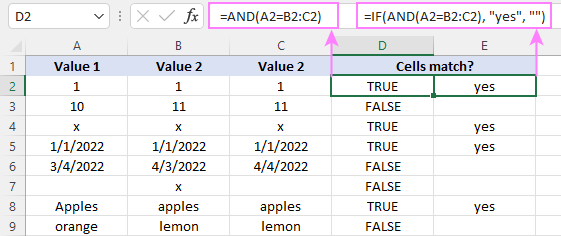
If two cells equal, return TRUE
The simplest «If one cell equals another then true» Excel formula is this:
For example, to compare cells in columns A and B in each row, you enter this formula in C2, and then copy it down the column:
As the result, you’ll get TRUE if two cells are the same, FALSE otherwise:

- This formula returns two Boolean values: if two cells are equal — TRUE; if not equal — FALSE. To only return the TRUE values, use in IF statement as shown in the next example.
- This formula is case-insensitive, so it treats uppercase and lowercase letters as the same characters. If the text case matters, then use this case-sensitive formula.
If two cells match, return value
To return your own value if two cells match, construct an IF statement using this pattern:
For example, to compare A2 and B2 and return «yes» if they contain the same values, «no» otherwise, the formula is:

If you only want to return a value if cells are equal, then supply an empty string («») for value_if_false.
If match, then yes:
If match, then TRUE:

Note. To return the logical value TRUE, don’t enclose it in double quotes. Using double quotes will convert the logical value into a regular text string.
If one cell equals another, then return another cell
And here’s a variation of the Excel if match formula that solves this specific task: compare the values in two cells and if the data match, then copy a value from another cell.
In the Excel language, it’s formulated like this:
For instance, to check the items in columns A and B and return a value from column C if text matches, the formula in D2, copied down, is:

Case-sensitive formula to see if two cells match
In situation when you are dealing with case-sensitive text values, use the EXACT function to compare the cells exactly, including the letter case:
For example, to compare the items in A2 and B2 and return «yes» if text matches exactly, «no» if any difference is found, you can use this formula:
=IF(EXACT(A2, B2), «Yes», «No»)

How to check if multiple cells are equal
As with comparing two cells, checking multiple cells for matches can also be done in a few different ways.
AND formula to see if multiple cells match
To check if multiple values match, you can use the AND function with two or more logical tests:
For example, to see if cells A2, B2 and C2 are equal, the formula is:
In dynamic array Excel (365 and 2021) you can also use the below syntax. In Excel 2019 and lower, this will only work as a traditional CSE array formula, completed by pressing the Ctrl + Shift + Enter keys together.
The result of both AND formulas is the logical values TRUE and FALSE.
To return your own values, wrap AND in the IF function like this:
This formula returns «yes» if all three cells are equal, a blank cell otherwise.
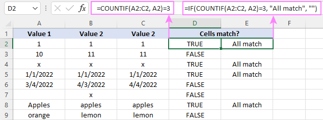
COUNTIF formula to check if multiple columns match
Another way to check for multiple matches is using the COUNTIF function in this form:
Where range is a range of cells to be compared against each other, cell is any single cell in the range, and n is the number of cells in the range.
For our sample dataset, the formula can be written in this form:
If you are comparing a lot of columns, the COLUMNS function can get the cells’ count (n) for you automatically:
And the IF function will help you return anything you want as an outcome:
=IF(COUNTIF(A2:C2, A2)=3, «All match», «»)
Case-sensitive formula for multiple matches
As with checking two cells, we employ the EXACT function to perform the exact comparison, including the letter case. To handle multiple cells, EXACT is to be nested into the AND function like this:
In Excel 365 and Excel 2021, due to support for dynamic arrays, this works as a normal formula. In Excel 2019 and lower, remember to press Ctrl + Shift + Enter to make it an array formula.
For example, to check if cells A2:C2 contain the same values, a case-sensitive formula is:
In combination with IF, it takes this shape:
=IF(AND(EXACT(A2:C2, A2)), «Yes», «No»)

Check if cell matches any cell in range
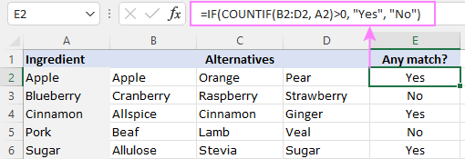
To see if a cell matches any cell in a given range, utilize one of the following formulas:
It’s best to be used for checking 2 — 3 cells.
Excel 365 and Excel 2021 understand this syntax as well:
In Excel 2019 and lower, this should be entered as an array formula by pressing the Ctrl + Shift + Enter shortcut.
For instance, to check if A2 equals any cell in B2:D2, any of these formulas will do:
=OR(A2=B2, A2=C2, A2=D2)
If you are using Excel 2019 or lower, remember to press Ctrl + Shift + Enter to get the second OR formula to deliver the correct results.
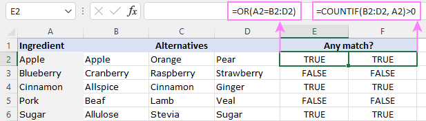
To return Yes/No or any other values you want, you know what to do — nest one of the above formulas in the logical test of the IF function. For example:
=IF(COUNTIF(B2:D2, A2)>0, «Yes», «No»)
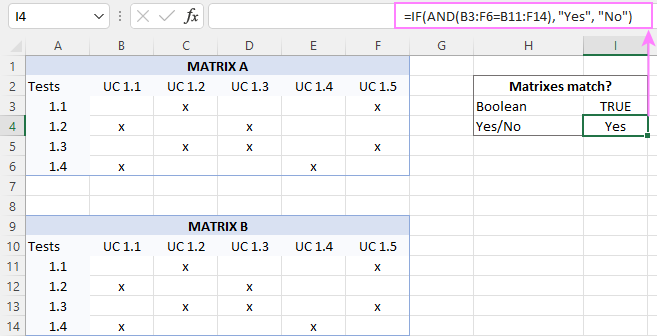
Check if two ranges are equal
To compare two ranges cell-by-cell and return the logical value TRUE if all the cells in the corresponding positions match, supply the equally sized ranges to the logical test of the AND function:
For example, to compare Matrix A in B3:F6 and Matrix B in B11:F14, the formula is:
To get Yes/No as the result, use the following IF AND combination:
=IF(AND(B3:F6=B11:F14), «Yes», «No»)
That’s how to use the If match formula in Excel. I thank you for reading and hope to see you on our blog next week!
Table of contents
Hi, I’m wanting to return a value if one cell equals another then put in say 10, otherwise leave blank. I have tried =if (d3=c3,10,””). If you leave both those cells blank it returns the 10 value which is not what I want. I want it to be blank but if those two cells are equal then I want the answer to be 10. Any help would be greatly appreciated.
To check if a cell is empty, you can use the function ISBLANK. For more information, please visit: ISBLANK function in Excel to check if cell is blank. Use the IF AND statement for multiple conditions.
If I understand your task correctly, try the following formula:
If cell 1 ,2 & 3 have values and are populated accordingly, then I want a Text string returned, for example «Matched» in a new column.
If cell 1 ,2 & 3 have no values and are not populated accordingly, then I want a Text string returned, for example «Unmatched» in a new column.
Hi!
Have you tried the ways described in this blog post? If they don’t work for you, then please describe your task in detail, explain what «populated accordingly» means.
I find a lot of this so informational! I have been scratching my head, but i’m trying to create a cell where if yes that Cell A says «Yes» based on a condition being met, and Cell B also says «Yes» on its own condition being met, that this formula will then read «Yes» indicating both conditions were met. Same if only one says YES and the other says No, this will read «no» and they must both be «YES» to end up as a yes? The issue i have is, if both cells conditions were not met and it says «no» the final cell is still indicating «true» since they match each other.
If that made sense to anyone.
Hi!
If I got you right, the formula below will help you with your task:
Wow. I am just speechless, Alexander. You are extremely skilled at this, and understand it so phenomenally! I can’t thank you enough for that!
I am comparing two columns and the individual columns have duplicated values. How can I match ? for example if one of the column have two 10,000 and the other column have three 10,000 I want to get one 10,000 as a difference.
I am working a pulling info and I was using vlookup and it work great =VLOOKUP(A2,’Employee Ben’!A$2:DE$1650,107,FALSE)
I can reference the ssn in the first column and then it searches the employee ben sheet for the number and then pulls the column that i ask for for the match. Problem is need to match 2 fields in the same row and and then pull a specified column. I cannot figure this out. Driving me Mad.
Hello!
To Vlookup multiple criteria, you can use either an INDEX MATCH combination with multiple criteria or the XLOOKUP function.
Is there a way to look at all (text) data in Column A, does it match a text value in Column B, and if ‘yes’ — enter what is in Column C into Column D.
Column B, C and D are all aligned in the same row.
hello
I want to ask if there is a possibility of compare the names in two rows where by in each row there are three for each person and the names but some of the names are not match exactly. If there is a possibility that at least two names to be match and the status became match
example
Mussa Jayden Ally vs Musa Jayden Ally
I need to see these match regardless of the difference in the name mussa vs musa
Hello!
You can split each text into 3 columns as described in this guide: How to split cells in Excel. Then compare the columns using these guidelines: Compare two columns for matches and differences.
Copyright © 2003 – 2023 Office Data Apps sp. z o.o. All rights reserved.
Microsoft and the Office logos are trademarks or registered trademarks of Microsoft Corporation. Google Chrome is a trademark of Google LLC.
Источник
Excel for Microsoft 365 Excel for Microsoft 365 for Mac Excel for the web Excel 2021 Excel 2021 for Mac Excel 2019 Excel 2019 for Mac Excel 2016 Excel 2016 for Mac Excel 2013 Excel for iPad Excel for iPhone Excel for Android tablets Excel 2010 Excel for Mac 2011 Excel for Android phones More…Less
Operators specify the type of calculation that you want to perform on the elements of a formula. There is a default order in which calculations occur, but you can change this order by using parentheses.
In this article
-
Types of operators
-
The order in which Excel performs operations in formulas
Types of operators
There are four different types of calculation operators: arithmetic, comparison, text concatenation (combining text), and reference.
Arithmetic operators
To perform basic mathematical operations such as addition, subtraction, or multiplication; combine numbers; and produce numeric results, use the following arithmetic operators in a formula:
|
Arithmetic operator |
Meaning |
Example |
Result |
|
+ (plus sign) |
Addition |
=3+3 |
6 |
|
– (minus sign) |
Subtraction |
=3–1 |
2 -1 |
|
* (asterisk) |
Multiplication |
=3*3 |
9 |
|
/ (forward slash) |
Division |
=15/3 |
5 |
|
% (percent sign) |
Percent |
=20%*20 |
4 |
|
^ (caret) |
Exponentiation |
=3^2 |
9 |
Comparison operators
You can compare two values with the following operators. When two values are compared by using these operators, the result is a logical value either TRUE or FALSE.
|
Comparison operator |
Meaning |
Example |
|
= (equal sign) |
Equal to |
A1=B1 |
|
> (greater than sign) |
Greater than |
A1>B1 |
|
< (less than sign) |
Less than |
A1<B1 |
|
>= (greater than or equal to sign) |
Greater than or equal to |
A1>=B1 |
|
<= (less than or equal to sign) |
Less than or equal to |
A1<=B1 |
|
<> (not equal to sign) |
Not equal to |
A1<>B1 |
Text concatenation operator
Use the ampersand (&) to concatenate (combine) one or more text strings to produce a single piece of text.
|
Text operator |
Meaning |
Example |
Result |
|
& (ampersand) |
Connects, or concatenates, two values to produce one continuous text value |
=»North»&»wind» |
Northwind |
|
=»Hello» & » » & «world» This example inserts a space character between the two words. The space character is specified by enclosing a space in opening and closing quotation marks (» «). |
Hello world |
Reference operators
Combine ranges of cells for calculations with the following operators.
|
Reference operator |
Meaning |
Example |
|
: (colon) |
Range operator, which produces one reference to all the cells between two references, including the two references |
B5:B15 |
|
, (comma) |
Union operator, which combines multiple references into one reference |
SUM(B5:B15,D5:D15) |
|
(space) |
Intersection operator, which returns a reference to the cells common to the ranges in the formula. In this example, cell C7 is found in both ranges, so it is the intersection. |
B7:D7 C6:C8 |
Top of Page
The order in which Excel performs operations in formulas
In some cases, the order in which calculation is performed can affect the return value of the formula, so it’s important to understand how the order is determined and how you can change the order to obtain desired results.
Calculation order
Formulas calculate values in a specific order. A formula in Excel always begins with an equal sign (=). The equal sign tells Excel that the characters that follow constitute a formula. Following the equal sign are the elements to be calculated (the operands, such as numbers or cell references), which are separated by calculation operators (such as +, -, *, or /). Excel calculates the formula from left to right, according to a specific order for each operator in the formula.
Operator precedence
If you combine several operators in a single formula, Excel performs the operations in the order shown in the following table. If a formula contains operators with the same precedence — for example, if a formula contains both a multiplication and division operator — Excel evaluates the operators from left to right.
|
Operator |
Description |
|
: (colon) (single space) , (comma) |
Reference operators |
|
– |
Negation (as in –1) |
|
% |
Percent |
|
^ |
Exponentiation (raising to a power) |
|
* and / |
Multiplication and division |
|
+ and – |
Addition and subtraction |
|
& |
Connects two strings of text (concatenation) |
|
= |
Comparison |
Use of parentheses
To change the order of evaluation, enclose in parentheses the part of the formula to be calculated first. For example, the following formula produces 11 because Excel calculates multiplication before addition. The formula multiplies 2 by 3 and then adds 5 to the result.
=5+2*3
In contrast, if you use parentheses to change the syntax, Excel adds 5 and 2 together and then multiplies the result by 3 to produce 21.
=(5+2)*3
In the following example, the parentheses around the first part of the formula force Excel to calculate B4+25 first and then divide the result by the sum of the values in cells D5, E5, and F5.
=(B4+25)/SUM(D5:F5)
Top of Page
Need more help?
Equal to | Greater than | Less than | Greater than or equal to | Less than or equal to | Not equal to
Use comparison operators in Excel to check if two values are equal to each other, if one value is greater than another value, if one value is less than another value, etc.
Equal to
The equal to operator (=) returns TRUE if two values are equal to each other.
1. For example, take a look at the formula in cell C1 below.
Explanation: the formula returns TRUE because the value in cell A1 is equal to the value in cell B1. Always start a formula with an equal sign (=).
2. The IF function below uses the equal to operator.
Explanation: if the two values (numbers or text strings) are equal to each other, the IF function returns Yes, else it returns No.
Greater than
The greater than operator (>) returns TRUE if the first value is greater than the second value.
1. For example, take a look at the formula in cell C1 below.
Explanation: the formula returns TRUE because the value in cell A1 is greater than the value in cell B1.
2. The OR function below uses the greater than operator.
Explanation: this OR function returns TRUE if at least one value is greater than 50, else it returns FALSE.
Less than
The less than operator (<) returns TRUE if the first value is less than the second value.
1. For example, take a look at the formula in cell C1 below.

Explanation: the formula returns TRUE because the value in cell A1 is less than the value in cell B1.
2. The AND function below uses the less than operator.

Explanation: this AND function returns TRUE if both values are less than 80, else it returns FALSE.
Greater than or equal to
The greater than or equal to operator (>=) returns TRUE if the first value is greater than or equal to the second value.
1. For example, take a look at the formula in cell C1 below.
Explanation: the formula returns TRUE because the value in cell A1 is greater than or equal to the value in cell B1.
2. The COUNTIF function below uses the greater than or equal to operator.
Explanation: this COUNTIF function counts the number of cells that are greater than or equal to 10.
Less than or equal to
The less than or equal to operator (<=) returns TRUE if the first value is less than or equal to the second value.
1. For example, take a look at the formula in cell C1 below.

Explanation: the formula returns TRUE because the value in cell A1 is less than or equal to the value in cell B1.
2. The SUMIF function below uses the less than or equal to operator.

Explanation: this SUMIF function sums values in the range A1:A5 that are less than or equal to 10.
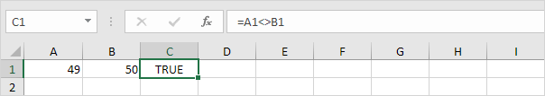
Not Equal to
The not equal to operator (<>) returns TRUE if two values are not equal to each other.
1. For example, take a look at the formula in cell C1 below.
Explanation: the formula returns TRUE because the value in cell A1 is not equal to the value in cell B1.
2. The IF function below uses the not equal to operator.
Explanation: if the two values (numbers or text strings) are not equal to each other, the IF function returns No, else it returns Yes.