
Enter data manually in worksheet cells
Excel for Microsoft 365 Excel 2021 Excel 2019 Excel 2016 Excel 2013 Excel 2010 Excel 2007 More…Less
You have several options when you want to enter data manually in Excel. You can enter data in one cell, in several cells at the same time, or on more than one worksheet at once. The data that you enter can be numbers, text, dates, or times. You can format the data in a variety of ways. And, there are several settings that you can adjust to make data entry easier for you.
This topic does not explain how to use a data form to enter data in worksheet. For more information about working with data forms, see Add, edit, find, and delete rows by using a data form.
Important: If you can’t enter or edit data in a worksheet, it might have been protected by you or someone else to prevent data from being changed accidentally. On a protected worksheet, you can select cells to view the data, but you won’t be able to type information in cells that are locked. In most cases, you should not remove the protection from a worksheet unless you have permission to do so from the person who created it. To unprotect a worksheet, click Unprotect Sheet in the Changes group on the Review tab. If a password was set when the worksheet protection was applied, you must first type that password to unprotect the worksheet.
-
On the worksheet, click a cell.
-
Type the numbers or text that you want to enter, and then press ENTER or TAB.
To enter data on a new line within a cell, enter a line break by pressing ALT+ENTER.
-
On the File tab, click Options.
In Excel 2007 only: Click the Microsoft Office Button
 , and then click Excel Options.
 -
Click Advanced, and then under Editing options, select the Automatically insert a decimal point check box.
-
In the Places box, enter a positive number for digits to the right of the decimal point or a negative number for digits to the left of the decimal point.
For example, if you enter 3 in the Places box and then type 2834 in a cell, the value will appear as 2.834. If you enter -3 in the Places box and then type 283, the value will be 283000.
-
On the worksheet, click a cell, and then enter the number that you want.
Data that you typed in cells before selecting the Fixed decimal option is not affected.
To temporarily override the Fixed decimal option, type a decimal point when you enter the number.
 , and then click Excel Options.
-
On the worksheet, click a cell.
-
Type a date or time as follows:
-
To enter a date, use a slash mark or a hyphen to separate the parts of a date; for example, type 9/5/2002 or 5-Sep-2002.
-
To enter a time that is based on the 12-hour clock, enter the time followed by a space, and then type a or p after the time; for example, 9:00 p. Otherwise, Excel enters the time as AM.
To enter the current date and time, press Ctrl+Shift+; (semicolon).
-
-
To enter a date or time that stays current when you reopen a worksheet, you can use the TODAY and NOW functions.
-
When you enter a date or a time in a cell, it appears either in the default date or time format for your computer or in the format that was applied to the cell before you entered the date or time. The default date or time format is based on the date and time settings in the Regional and Language Options dialog box (Control Panel, Clock, Language, and Region). If these settings on your computer have been changed, the dates and times in your workbooks that have not been formatted by using the Format Cells command are displayed according to those settings.
-
To apply the default date or time format, click the cell that contains the date or time value, and then press Ctrl+Shift+# or Ctrl+Shift+@.
-
Select the cells into which you want to enter the same data. The cells do not have to be adjacent.
-
In the active cell, type the data, and then press Ctrl+Enter.
You can also enter the same data into several cells by using the fill handle
to automatically fill data in worksheet cells.For more information, see the article Fill data automatically in worksheet cells.
 to automatically fill data in worksheet cells.
By making multiple worksheets active at the same time, you can enter new data or change existing data on one of the worksheets, and the changes are applied to the same cells on all the selected worksheets.
-
Click the tab of the first worksheet that contains the data that you want to edit. Then hold down Ctrl while you click the tabs of other worksheets in which you want to synchronize the data.
Note: If you don’t see the tab of the worksheet that you want, click the tab scrolling buttons to find the worksheet, and then click its tab. If you still can’t find the worksheet tabs that you want, you might have to maximize the document window.
-
On the active worksheet, select the cell or range in which you want to edit existing or enter new data.
-
In the active cell, type new data or edit the existing data, and then press Enter or Tab to move the selection to the next cell.
The changes are applied to all the worksheets that you selected.
-
Repeat the previous step until you have completed entering or editing data.

-
To cancel a selection of multiple worksheets, click any unselected worksheet. If an unselected worksheet is not visible, you can right-click the tab of a selected worksheet, and then click Ungroup Sheets.
-
When you enter or edit data, the changes affect all the selected worksheets and can inadvertently replace data that you didn’t mean to change. To help avoid this, you can view all the worksheets at the same time to identify potential data conflicts.
-
On the View tab, in the Window group, click New Window.
-
Switch to the new window, and then click a worksheet that you want to view.
-
Repeat steps 1 and 2 for each worksheet that you want to view.
-
On the View tab, in the Window group, click Arrange All, and then click the option that you want.
-
To view worksheets in the active workbook only, in the Arrange Windows dialog box, select the Windows of active workbook check box.
-
There are several settings in Excel that you can change to help make manual data entry easier. Some changes affect all workbooks, some affect the whole worksheet, and some affect only the cells that you specify.
Change the direction for the Enter key
When you press Tab to enter data in several cells in a row and then press Enter at the end of that row, by default, the selection moves to the start of the next row.
Pressing Enter moves the selection down one cell, and pressing Tab moves the selection one cell to the right. You cannot change the direction of the move for the Tab key, but you can specify a different direction for the Enter key. Changing this setting affects the whole worksheet, any other open worksheets, any other open workbooks, and all new workbooks.
-
On the File tab, click Options.
In Excel 2007 only: Click the Microsoft Office Button
, and then click Excel Options. -
In the Advanced category, under Editing options, select the After pressing Enter, move selection check box, and then click the direction that you want in the Direction box.
Change the width of a column
At times, a cell might display #####. This can occur when the cell contains a number or a date and the width of its column cannot display all the characters that its format requires. For example, suppose a cell with the Date format «mm/dd/yyyy» contains 12/31/2015. However, the column is only wide enough to display six characters. The cell will display #####. To see the entire contents of the cell with its current format, you must increase the width of the column.
-
Click the cell for which you want to change the column width.
-
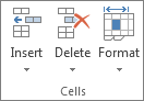
On the Home tab, in the Cells group, click Format.
-
Under Cell Size, do one of the following:
-
To fit all text in the cell, click AutoFit Column Width.
-
To specify a larger column width, click Column Width, and then type the width that you want in the Column width box.
-
Note: As an alternative to increasing the width of a column, you can change the format of that column or even an individual cell. For example, you could change the date format so that a date is displayed as only the month and day («mm/dd» format), such as 12/31, or represent a number in a Scientific (exponential) format, such as 4E+08.
Wrap text in a cell
You can display multiple lines of text inside a cell by wrapping the text. Wrapping text in a cell does not affect other cells.
-
Click the cell in which you want to wrap the text.
-
On the Home tab, in the Alignment group, click Wrap Text.
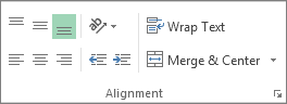
Note: If the text is a long word, the characters won’t wrap (the word won’t be split); instead, you can widen the column or decrease the font size to see all the text. If all the text is not visible after you wrap the text, you might have to adjust the height of the row. On the Home tab, in the Cells group, click Format, and then under Cell Size click AutoFit Row.
For more information on wrapping text, see the article Wrap text in a cell.
Change the format of a number
In Excel, the format of a cell is separate from the data that is stored in the cell. This display difference can have a significant effect when the data is numeric. For example, when a number that you enter is rounded, usually only the displayed number is rounded. Calculations use the actual number that is stored in the cell, not the formatted number that is displayed. Hence, calculations might appear inaccurate because of rounding in one or more cells.
After you type numbers in a cell, you can change the format in which they are displayed.
-
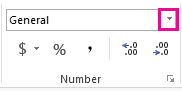
Click the cell that contains the numbers that you want to format.
-
On the Home tab, in the Number group, click the arrow next to the Number Format box, and then click the format that you want.
To select a number format from the list of available formats, click More Number Formats, and then click the format that you want to use in the Category list.
Format a number as text
For numbers that should not be calculated in Excel, such as phone numbers, you can format them as text by applying the Text format to empty cells before typing the numbers.
-
Select an empty cell.
-
On the Home tab, in the Number group, click the arrow next to the Number Format box, and then click Text.
-
Type the numbers that you want in the formatted cell.
Numbers that you entered before you applied the Text format to the cells must be entered again in the formatted cells. To quickly reenter numbers as text, select each cell, press F2, and then press Enter.
Need more help?
You can always ask an expert in the Excel Tech Community or get support in the Answers community.
Need more help?
Once you know how to enter data into an Excel worksheet you will be setting up tables of data in no time.
When you haven’t been shown how to enter data it can be a little tricky, so follow the steps below to learn the tips and hacks to entering your data easily into your worksheet.
Entering data into an Excel worksheet
You can enter either values (numbers and dates) or labels (text) into any cell within the worksheet.
1. Move the cell pointer to the required cell and then type the data. While you type the data you will notice that it appears both in the worksheet (in the example below, the text appears in cell A1) and in the Formula Bar.
2. Press ENTER to enter the information into the cell. Your cell pointer will move down to the cell below.
Tip: If you press the ESC key instead of ENTER the data will not be entered into the cell.
Deleting and replacing data
- To delete data select the cell containing the data and then press DELETE.
- To replace data just type directly over the top of the existing cell contents. The new data will replace the old.
Using Undo and Redo
There will be times when you enter data only to realise you have made a bit of a mess of things.
Most times you want to back-back to where you were before the mistake was made. If this happens you can click the fabulous “Undo” button which will undo the last thing you did.
You can actually keep clicking it until you get back to a point where you feel in control again.
And if you go one step to far back, you can click the Redo button to go forward a step again. These buttons are fabulous and you use them a lot.
Overlapping data
If you enter data that will not fit the column width it will overlap into the next column. In the example below the text ‘Travel Expenses’ is entered into cell A1, however it looks as though the text is included in cells B1. With cell A1 selected we can see in the Formula bar that both words are indeed in A1.
If you are not using the column into which the text is overlapping you may leave the text as it is. However, as soon as you place text into a cell that has been overlapped it will look as if your text has been lost. In the example below, the text ‘Amount ex GST’ has been entered into cell C3. However the content of cell D3 is hiding part of the content is C3.
By selecting C3 the entire cell’s content can be seen in the Formula Bar. In order to view the entire contents of cell C3 the width of column C needs to be adjusted.
Working with columns
The standard column width for Excel is 8.43 character spaces. You can change the column width by dragging with your mouse on the column headers, or by double clicking between two column headers.
Tip: If multiple columns require the same width, select the columns and widen one of them with the mouse. The rest will be adjusted to the same width.
Adjusting the column width
To use your mouse to adjust the column width:
1. Move your mouse pointer over the column’s right edge in the column header area. Your mouse pointer should change to a double-headed arrow.
2. Click and drag to the right to expand, or to the left to shrink the column width to the size you require.
You will now be able to see your entire text. Continue dragging until all columns are the width you require.
Tips:
To quickly adjust the column width to fit the widest entry, move your mouse pointer over the lines between the column headers. When the pointer becomes a double-headed arrow double-click.
Use the same method for adjusting the height of any row. Just move the mouse pointer over the line separating the rows. When the pointer becomes a double-headed arrow, drag or double-click to adjust the row height, or double-click to set the height to fit the tallest entry.
By the way, row heights will automatically alter if the font size of data is altered.
Extra info: to set a column width to a precise measurement on the Home tab in the Cells group select Format and then select Column Width. Type the desired width in the Column Width box and then click OK to accept the new column width.
What do hash signs mean in Excel?
If you ever see a cell containing ######## (hash signs) it means the column isn’t wide enough to display the content. Just extend the width and the content will become visible.
Making changes to the data
Once you have entered data into your worksheet, you can edit the data in a number of ways.
- Select the cell and then click in the Formula bar. A flashing insertion point will be placed into the bar. Use the arrow keys on the keyboard to move the insertion point. Make the changes you require and then press ENTER.
- You may also type directly over the data in the cell with new data and then press ENTER. The new data will replace the old.
- Double clicking a cell or pressing F2 allows you to edit the contents of the cell directly on the worksheet. Make the changes and then press ENTER to update the cell.
AutoComplete
AutoComplete is the ability for Excel to automatically complete an entry for you.
For example, if you have typed text in the cells above as soon as you start typing a letter or two in a cell below, Excel will check the list above for a matching entry and complete the entry for you.
This can be very useful when you need to make the same entry several times.
To accept the entry press ENTER. To reject the displayed entry and type something different either ignore the entry and type right over it or press DELETE.
Was this blog helpful? Let us know in the Comments below.
Instructions
Entering data into an Excel worksheet
- Move the cell pointer to the required cell and then type the data.
- Press ENTER to enter the information into the cell. Your cell pointer will move down to the cell below.
Deleting and replacing data
To Delete: Select the cell containing the data and then press DELETE.
To replace data: Type directly over the top of the existing cell contents. The new data will replace the old.
Using Undo and Redo
If you make a mistake, you can use the Undo button on the top right of the Excel spreadsheet to undo the last thing you did. You can keep clicking it to go back multiple steps.
If you Undo something you didn’t want undone, you can use the Redo button to the right of the Undo button to go forward a step again.
Overlapping data
If you enter data that will not fit the column width it will overlap into the next column. Adjust the width of the columns in order to view the entire contents.
Working with columns
Adjusting the column width
- Move your mouse pointer over the column’s right edge in the column header area. Your mouse pointer should change to a double-headed arrow.
- Click and drag to the right to expand, or to the left to shrink the column width to the size you require.
- You will now be able to see your entire text. Continue dragging until all columns are the width you require.
Making changes to the data
- Select the cell and then click in the Formula bar. A flashing insertion point will be placed into the bar. Use the arrow keys on the keyboard to move the insertion point. Make the changes you require and then press ENTER.
- You may also type directly over the data in the cell with new data and then press ENTER. The new data will replace the old.
- Double clicking a cell or pressing F2 allows you to edit the contents of the cell directly on the worksheet. Make the changes and then press ENTER to update the cell.
AutoComplete
Sometimes when you are typing in a cell, Excel will automatically complete the entry for you. To accept the entry press ENTER. To reject the displayed entry and type something different either ignore the entry and type right over it or press DELETE.
Notes
Note: While you type the data you will notice that it appears both in the worksheet cell and in the Formula Bar.
Tip: If you press the ESC key instead of ENTER when typing data into a cell the data will not be entered into the cell.
Tips: To quickly adjust the column width to fit the widest entry, move your mouse pointer over the lines between the column headers. When the pointer becomes a double-headed arrow double-click.
Extra info: to set a column width to a precise measurement on the Home tab in the Cells group select Format and then select Column Width. Type the desired width in the Column Width box and then click OK to accept the new column width.
Note: If you ever see a cell containing ######## (hash signs) it means the column isn’t wide enough to display the content. Just extend the width and the content will become visible.
Watch the Video on Using Data Entry Forms in Excel
Below is a detailed written tutorial about Excel Data Entry form in case you prefer reading over watching a video.
Excel has many useful features when it comes to data entry.
And one such feature is the Data Entry Form.
In this tutorial, I will show you what are data entry forms and how to create and use them in Excel.
Why Do You Need to Know About Data Entry Forms?
Maybe you don’t!
But if data entry is a part of your daily work, I recommend you check out this feature and see how it can help you save time (and make you more efficient).
There are two common issues that I have faced (and seen people face) when it comes to data entry in Excel:
- It’s time-consuming. You need to enter the data in one cell, then go to the next cell and enter the data for it. Sometimes, you need to scroll up and see which column it is and what data needs to be entered. Or scroll to the right and then come back to the beginning in case there are many columns.
- It’s error-prone. If you have a huge data set which needs 40 entries, there is a possibility you may end up entering something that was not intended for that cell.
A data entry form can help by making the process faster and less error-prone.
Before I show you how to create a data entry form in Excel, let me quickly show you what it does.
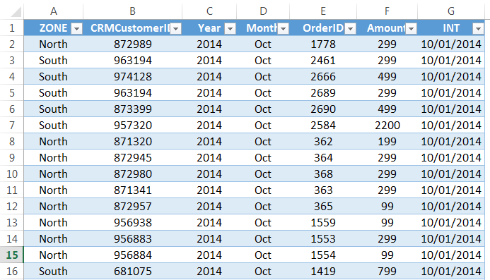
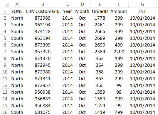
Below is a data set that is typically maintained by the hiring team in an organization.
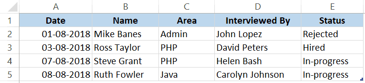
Every time a user has to add a new record, he/she will have to select the cell in the next empty row and then go cell by cell to make the entry for each column.
While this is a perfectly fine way of doing it, a more efficient way would be to use a Data Entry Form in Excel.
Below is a data entry form that you can use to make entries to this data set.
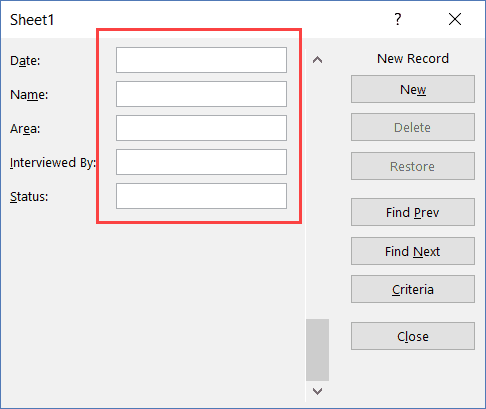
The highlighted fields are where you would enter the data. Once done, hit the Enter key to make the data a part of the table and move on to the next entry.
Below is a demo of how it works:
As you can see, this is easier than regular data entry as it has everything in a single dialog box.
Data Entry Form in Excel
Using a data entry form in Excel needs a little pre-work.
You would notice that there is no option to use a data entry form in Excel (not in any tab in the ribbon).
To use it, you will have to first add it to the Quick Access Toolbar (or the ribbon).
Adding Data Entry Form Option To Quick Access Toolbar
Below are the steps to add the data entry form option to the Quick Access Toolbar:
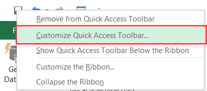
- Right-click on any of the existing icons in the Quick Access Toolbar.
- Click on ‘Customize Quick Access Toolbar’.

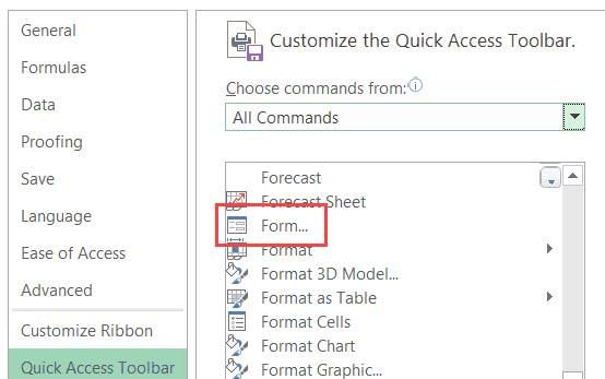
- In the ‘Excel Options’ dialog box that opens, select the ‘All Commands’ option from the drop-down.

- Scroll down the list of commands and select ‘Form’.

- Click on the ‘Add’ button.

- Click OK.


The above steps would add the Form icon to the Quick Access Toolbar (as shown below).
![]()
Once you have it in QAT, you can click any cell in your dataset (in which you want to make the entry) and click on the Form icon.
Note: For Data Entry Form to work, your data should be in an Excel Table. If it isn’t already, you’ll have to convert it into an Excel Table (keyboard shortcut – Control + T).
Parts of the Data Entry Form
A Data Entry Form in Excel has many different buttons (as you can see below).
Here is a brief description of what each button is about:
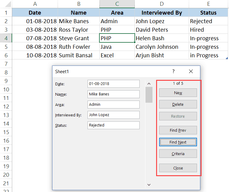
- New: This will clear any existing data in the form and allows you to create a new record.
- Delete: This will allow you to delete an existing record. For example, if I hit the Delete key in the above example, it will delete the record for Mike Banes.
- Restore: If you’re editing an existing entry, you can restore the previous data in the form (if you haven’t clicked New or hit Enter).
- Find Prev: This will find the previous entry.
- Find Next: This will find the next entry.
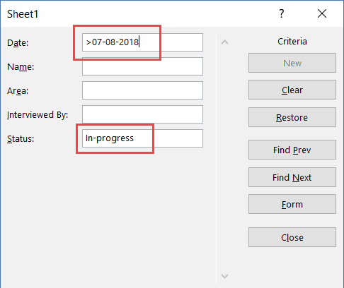
- Criteria: This allows you to find specific records. For example, if I am looking for all the records, where the candidate was Hired, I need to click the Criteria button, enter ‘Hired’ in the Status field and then use the find buttons. Example of this is covered later in this tutorial.
- Close: This will close the form.
- Scroll Bar: You can use the scroll bar to go through the records.
Now let’s go through all the things you can do with a Data Entry form in Excel.
Note that you need to convert your data into an Excel Table and select any cell in the table to be able to open the Data Entry form dialog box.
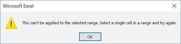
If you haven’t selected a cell in the Excel Table, it will show a prompt as shown below:
Creating a New Entry
Below are the steps to create a new entry using the Data Entry Form in Excel:
- Select any cell in the Excel Table.
- Click on the Form icon in the Quick Access Toolbar.

- Enter the data in the form fields.
- Hit the Enter key (or click the New button) to enter the record in the table and get a blank form for next record.
Navigating Through Existing Records
One of the benefits of using Data Entry Form is that you can easily navigate and edit the records without ever leaving the dialog box.
This can be especially useful if you have a dataset with many columns. This can save you a lot of scrolling and the process of going back and forth.
Below are the steps to navigate and edit the records using a data entry form:
- Select any cell in the Excel Table.
- Click on the Form icon in the Quick Access Toolbar.
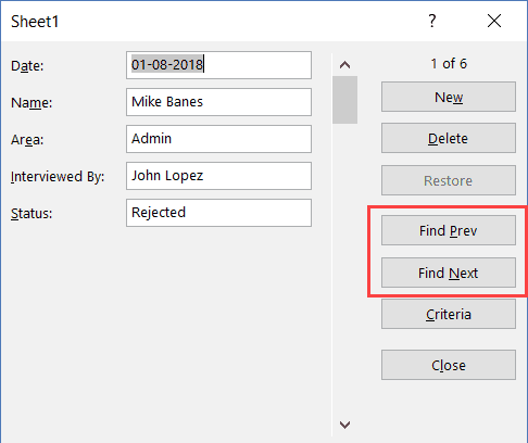
- To go to the next entry, click on the ‘Find Next’ button and to go to the previous entry, click the ‘Find Prev’ button.

- To edit an entry, simply make the change and hit enter. In case you want to revert to the original entry (if you haven’t hit the enter key), click the ‘Restore’ button.
You can also use the scroll bar to navigate through entries one-by-one.
The above snapshot shows basic navigation where you are going through all the records one after the other.
But you can also quickly navigate through all the records based on criteria.
For example, if you want to go through all the entries where the status is ‘In-progress’, you can do that using the below steps:
Criteria is a very useful feature when you have a huge dataset, and you want to quickly go through those records that meet a given set of criteria.
Note that you can use multiple criteria fields to navigate through the data.
For example, if you want to go through all the ‘In-progress’ records after 07-08-2018, you can use ‘>07-08-2018’ in the criteria for ‘Date’ field and ‘In-progress’ as the value in the status field. Now when you navigate using Find Prev/Find Next buttons, it will only show records after 07-08-2018 where the status is In-progress.
You can also use wildcard characters in criteria.
For example, if you have been inconsistent in entering the data and have used variations of a word (such as In progress, in-progress, in progress, and inprogress), then you need to use wildcard characters to get these records.
Below are the steps to do this:
- Select any cell in the Excel table.
- Click on the Form icon in the Quick Access Toolbar.
- Click the Criteria button.
- In the Status field, enter *progress
- Use the Find Prev/Find Next buttons to navigate through the entries where the status is In-Progress.

This works as an asterisk (*) is a wildcard character that can represent any number of characters in Excel. So if the status contains the ‘progress’, it will be picked up by Find Prev/Find Next buttons no matter what is before it).
Deleting a Record
You can delete records from the Data Entry form itself.
This can be useful when you want to find a specific type of records and delete these.
Below are the steps to delete a record using Data Entry Form:
- Select any cell in the Excel table.
- Click on the Form icon in the Quick Access Toolbar.
- Navigate to the record you want to delete
- Click the Delete button.

While you may feel that this all looks like a lot of work just to enter and navigate through records, it saves a lot of time if you’re working with lots of data and have to do data entry quite often.
Restricting Data Entry Based on Rules
You can use data validation in cells to make sure the data entered conforms to a few rules.
For example, if you want to make sure that the date column only accepts a date during data entry, you can create a data validation rule to only allow dates.
If a user enters a data that is not a date, it will not be allowed and the user will be shown an error.
Here is how to create these rules when doing data entry:
- Select the cells (or even the entire column) where you want to create a data validation rule. In this example, I have selected column A.
- Click the Data tab.

- Click the Data Validation option.

- In the ‘Data Validation’ dialog box, within the ‘Settings’ tab, select ‘Date’ from the ‘Allow’ drop down.

- Specify the start and the end date. Entries within this date range would be valid and rest all would be denied.
- Click OK.


Now, if you use the data entry form to enter data in the Date column, and if it isn’t a date, then it will not be allowed.
You will see a message as shown below:
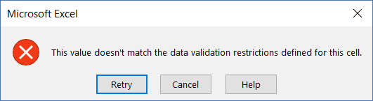
Similarly, you can use data validation with data entry forms to make sure users don’t end up entering the wrong data. Some examples where you can use this is numbers, text length, dates, etc.
Here are a few important things to know about Excel Data Entry Form:
- You can use wildcard characters while navigating through the records (through criteria option).
- You need to have an Excel table to be able to use the Data Entry Form. Also, you need to have a cell selected in it to use the form. There is one exception to this though. If you have a named range with the name ‘Database’, then the Excel Form will also refer to this named range, even if you have an Excel table.
- The field width in the Data Entry form is dependent on the column width of the data. If your column width is too narrow, the same would be reflected in the form.
- You can also insert bullet points in the data entry form. To do this, use the keyboard shortcut ALT + 7 or ALT + 9 from your numeric keypad. Here is a video about bullet points.
You May Also Like the Following Excel Tutorials:
- 100+ Excel Interview Questions.
- Drop Down Lists in Excel.
- Find and Remove Duplicates in Excel.
- Excel Text to Columns.
There is more than one way to enter data into an Excel worksheet. Sometimes we stick to typing directly into cells, but there are different ways to enter data which can speed up your data entry work.
- Type directly into a cell and add your data. You know a cell is active as it is highlighted with a darker border.

A2 is the active cell – it has a darker border so it stands out from the other cells - Use the formula bar. This is located under the ribbon. Type your data directly into the formula bar and press enter. You can navigate around the worksheet by typing the cell number directly into the Name box (located above the Column headings A – Z).

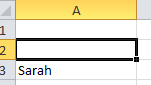
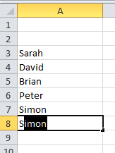
The Name Box shows that the active cell is A3. - Make the most of autocomplete. Excel will try to help you speed up your data entry by guessing what you are typing based on what’s in your worksheet. If the autocorrect option is right for you, just press enter.

Autocomplete is guessing that I am typing Simon, and I’ve just typed “Si”, I can press enter and the full name is entered for me. - Copy and paste – you may have cells that you can copy and paste data within the same worksheet – it can save you time formatting a sheet, or you can copy data to another worksheet within the workbook.
- Let Autofill do the work. Autofill options can complete series of data, whether it is text or numbers. This saves lots of data entry when setting up worksheets, or entering data.

Computer Excel training can give you extra skills so you can speed up entering the data, so you can concentrate on using the information you’ve gathered. https://www.stl-training.co.uk/excel-2007-introduction.php
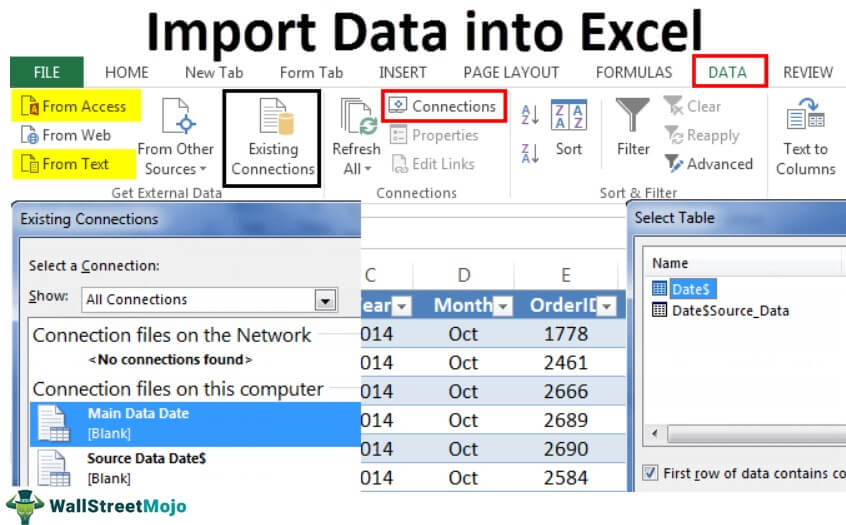
How to Import Data in Excel?
Importing the data from another file or another source file is often required in Excel. For example, sometimes people need data directly from very complicated servers, and sometimes we may need to import data from a text file or even from an Excel workbook.
If you are new to Excel data importing, then in this article, we will take a tour of importing data from text files, different Excel workbooks, and MS Access. Follow this article to learn the process involved in importing the data.
Table of contents
- How to Import Data in Excel?
- #1 – Import Data from Another Excel Workbook
- #2 – Import Data from MS Access to Excel
- #3 – Import Data from Text File to Excel
- Things to Remember
- Recommended Articles
#1 – Import Data from Another Excel Workbook
You can download this Import Data Excel Template here – Import Data Excel Template
Let us start.
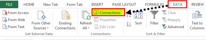
- First, we must go to the DATA tab. Then, under the DATA tab, click on Connections.

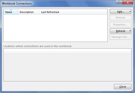
- As soon as we click on Connections, we may see the below window separately.

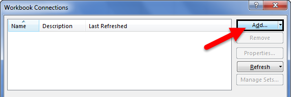
- Now, click on Add.

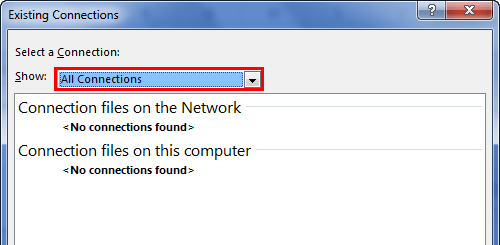
- It will open up a new window. In the below window, select All Connections.

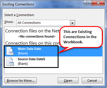
- If there are any connections in this workbook, it will show what those connections are here.

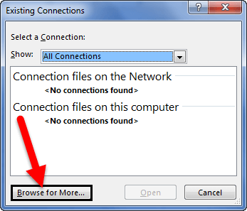
- Since we are connecting to a new workbook, click on Browse for more.

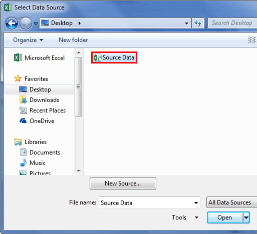
- In the below window, browse the file location. Then, click on Open.

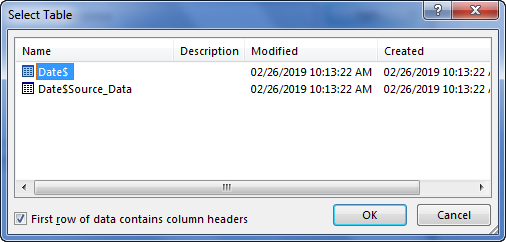
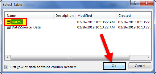
- After clicking on Open, it shows the below window.

- Here, we need to select the required table to be imported to this workbook. Select the table and click on OK.
After clicking on OK, close the Workbook Connection window.
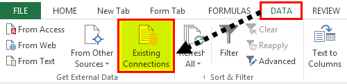
- Then, go to Existing Connections under the DATA tab.

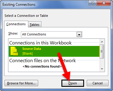
- Here, we will see all the existing connections. Select the connection we have just made and click on Open.

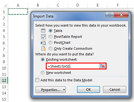
- Once we click on Open, it will ask us where to import the data. First, we need to select the cell reference here. Then, click on the OK button.

- It will import the data from the selected or connected workbook.

Like this, we can connect to the other workbook and import the data.
#2 – Import Data from MS Access to Excel
MS Access is the main platform to store the data safely. We can import the data directly from the MS Access File itself whenever the data is required.
Step 1: Go to the “DATA” ribbon in excelThe ribbon is an element of the UI (User Interface) which is seen as a strip that consists of buttons or tabs; it is available at the top of the excel sheet. This option was first introduced in the Microsoft Excel 2007.read more and select “From Access.“
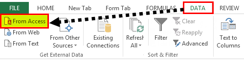
Step 2: Now, it will ask us to locate the desired file. Select the desired file path. Then, click on “Open.”
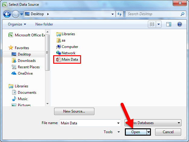
Step 3: Now, it will ask us to select the desired destination cell where we want to import the data. Then, click on “OK.”
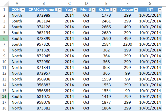
Step 4: It will import the data from access to the A1 cell in Excel.
#3 – Import Data from Text File to Excel
In almost all the corporations, whenever we ask for the data from the IT team, they will write a query and get the file in TEXT format. But unfortunately, TEXT file data is not the ready format to use in Excel; we need to make some modifications to work on it.
Step 1: Go to the “DATA” tab and click on “From Text.”

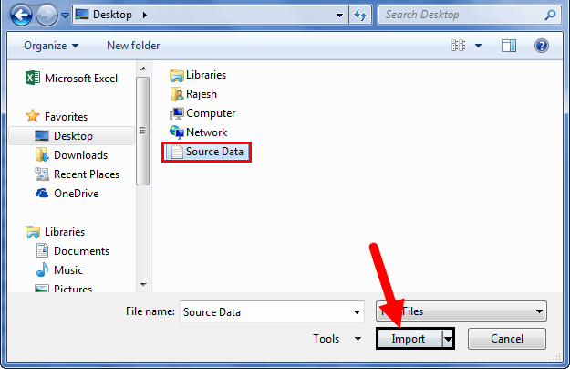
Step 2: Now, it will ask us to choose the file location on the computer or laptop. Select the targeted file, then click on “Import.”
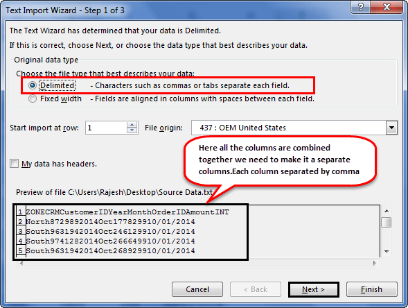
Step 3: It will open up a “Text Import Wizard.”
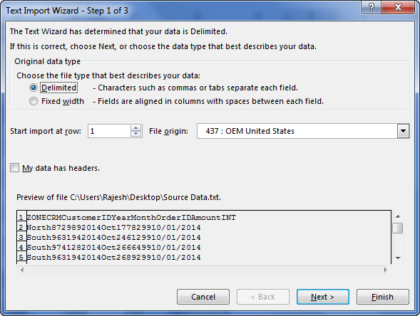
Step 4: By selecting the “Delimited,” click on “Next.”
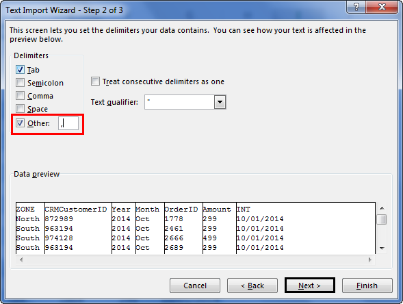
Step 5: In the next window, select the other and mention comma (,) because, in the text file, each column is separated by a comma (,). Then click on “Next.”
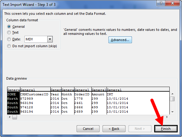
Step 6: In the next window, click on “Finish.”
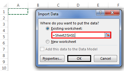
Step 7: Now, it will ask us to select the desired destination cell where we want to import the data. Select the cell and click on “OK.”
Step 8: It will import the data from the text file to the A1 cell in Excel.
Things to Remember
- If there are many tables, we must specify which table data we need to import.
- If we want the data in the current worksheet, we need to select the desired cell. Else, if we need data in a new worksheet, we must choose the new worksheet as the option.
- We need to separate the column in the TEXT file by identifying the common column separators.
Recommended Articles
This article is a guide to Import Data in Excel. Here, we discuss how to import data from 1) Excel Workbook, 2) MS Access, 3) Text File, practical examples, and a downloadable Excel template. You may learn more about Excel from the following articles: –
- KPI Dashboard in Excel
- Insert Image in Excel Cell
- How to Insert New Worksheet In Excel?
- Create a Dashboard in Excel
- Page Numbers in Excel
Entering data into Excel is exactly the same across all Excel versions and can be done in a number of different ways.
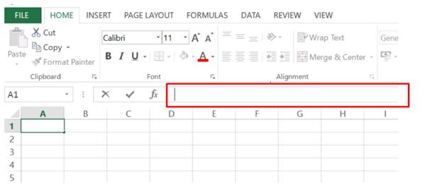
The first way you can enter data into Excel is using the formula bar. First you click on a cell, A1 for example and then you click on the formula bar so that the cursor appears within it.
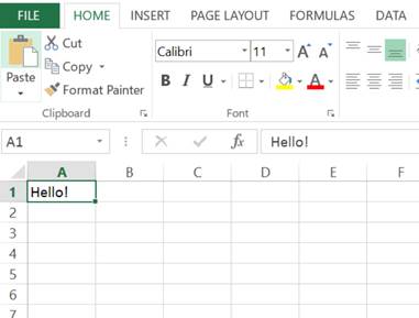
You can now type using the keyboard to enter data into cell A1. I typed Hello! into the formula bar and it also appears in the cell I had selected (A1):
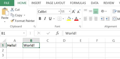
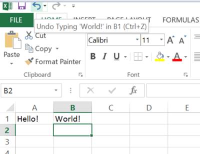
This also works by typing directly into the selected cell (without clicking on the formula bar). So if I select cell B2 and type World! it appears in the selected cell and the formula bar in exactly the same way:
If you dont like what youve typed into a particular cell you can undo the action much like in Word and other Office programs. This is done by clicking the Undo button. This is the backwards pointing arrow in the top left corner of Excel. By hovering the mouse over this button the undo action that will be performed is shown. So as the last thing I did was type World! into cell B1, clicking the undo button will remove world from cell B1.
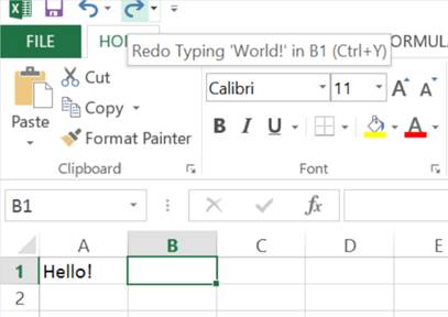
In addition to the Undo button there is also the Redo button. This is the forward pointing arrow and this re-does what you have just undone with the Undo button. So as I just used Undo to remove World! from cell B2, the Redo button will re-enter World! into cell B2.
Alternatively I could have used the keyboard shortcut Ctrl + Z to undo and Ctrl + Y to redo. These work the exact same way as clicking the buttons.
The Ctrl + Y shortcut for redo has some additional functionality. It can be used to repeat actions such as copying formats to other cells. I will go through how this feature works in more detail in the next tutorial as it saves time when making changes to individual or groups of cells.
![]()
Excel VBA Course — From Beginner to Expert
200+ Video Lessons
50+ Hours of Instruction
200+ Excel Guides
Become a master of VBA and Macros in Excel and learn how to automate all of your tasks in Excel with this online course. (No VBA experience required.)
View Course
Similar Content on TeachExcel
Use a Form to Enter Data into a Table in Excel
Tutorial:
You can enter data into a table in Excel using a form; here I’ll show you how to do that….
Put Data into a UserForm
Tutorial: How to take data from Excel and put it into a UserForm. This is useful when you use a form…
Put Data into a Worksheet using a Macro in Excel
Tutorial: How to input data into cells in a worksheet from a macro.
Once you have data in your macro…
VBA Macro to Import Web Data into Excel
Tutorial:
It’s time to learn how to use VBA and Macros to import data from a web page into Excel!
T…
How to Use Dates in Excel
Tutorial:
Introduction Guide to using Dates in Excel — this tutorial will show you how to input and…
Simple Alternatives to UserForms
Tutorial: This tutorial covers a few simple ways to show pop-up windows to users that allows you to …
Subscribe for Weekly Tutorials
BONUS: subscribe now to download our Top Tutorials Ebook!
![]()
Excel VBA Course — From Beginner to Expert
200+ Video Lessons
50+ Hours of Video
200+ Excel Guides
Become a master of VBA and Macros in Excel and learn how to automate all of your tasks in Excel with this online course. (No VBA experience required.)
View Course
Entering data in Excel is the same as typing text and numbers into the cells in an Excel worksheet. Formatting data in Excel is a process of modifying and customizing the texts and numbers entered.
As discussed in Microsoft Excel Tutorial 1, a cell is an intersection between a column label and a row number. This box has a reference or an address that is referred to when performing computations and analysis.
Before we can analyze or compute data in MS Excel, we must first enter the necessary data row-wise or column-wise. Depending on the nature of the analysis, formatting data and cells may be necessary.
In this tutorial, we shall look at how to enter and format data in an excel worksheet.
Entering data in Microsoft Excel can be done in three major ways:
- By typing in data into individual cells in an Excel worksheet,
- By copying and pasting data from another source to selected cells in a worksheet
- By importing data from an external data source
Enter data in a row or column
Microsoft Excel workspace, otherwise called worksheet is organized in columns and rows. To enter data by typing, you can arrange your data in a row or a column as shown below.

Then, you start typing on the first cell and arrange your column headings on the first row. Continue entering data on the cells below each column heading as you wish until you are done.
How you enter your data depends on the nature and purpose of the data. For more information on data entry in Excel, visit this post: Data Entry in Excel.
Using the fill command
When entering values in Microsoft Excel, you can fill in similar values and formulas across selected rows or columns automatically. This will save you the time and stress of typing similar data into the appropriate cells.
This fill command can be used manually or automatically. To use the manual fill command, do the following:
- Enter the data or formula in the first cell in a column or row.
- If it is a constant, e.g., 15, …, enter 15 in the first cell in a column or row.
- If it is a series, e.g., 1,2,…, enter the first two values in adjacent cells.
- Highlight the cell(s) with the values.
- You will see a small box in the bottom right of the highlighted cell(s).

- Click and drag the box downwards or rightwards to fill in values across columns or rows.
If you find it difficult to use this method, you can use the fill command on the Editing group as follow:
- Type the first value in a selected cell, and select that cell
- If you want to fill the same value across columns or rows, then, highlight a range of cells

- On the Home tab, under Editing group, select Fill.
- From the fill dropdown menu, select any of Down, Right, Up, or Left.
- If you want to fill series of values different from each other, thenuse the Series dialog box.
- On the Fill dropdownmenu, select Series, a dialog box will appear.

- On the dialog box, select Rows or Columns to specify where the values will fill across.
- Select Linear under Type and indicate a step and a stop value. You can choose any other type (growth, date, etc.) depending on your need.
- Click Ok, when you are done. The selected series will be filled automatically across the selected cells.
Copy and paste data in selected cells
You can also enter data in Microsoft Excel by copying from another source and pasting it in a worksheet. This method can be easily achieved by using the clipboard. See how to use the clipboard in our post on: Inserting and Formatting Texts.
To copy and paste data in Excel, do the following:
- Locate the source of the data.
- When the data source is opened, select the required data and press CTRL+C on the keyboard.
- Open the worksheet where you want to paste the data.
- Select a cell in the worksheet. The selected cell will mark the starting location to paste the data.
- If you want the data to be placed in a particular range, then select the range.
- On the Home tab, under the Clipboard group, click Paste. You can also press the CTRL+V key on the Keyboard.
The paste special command
Microsoft Excel gives you different paste options called paste special. When you copy or cut an item in Excel, you have the option to choose from different paste types.
There are about 14 different options namely:

- Paste: This option is used to paste the copied item(s) using default settings.
- Paste formula: This option is used to paste formulas in selected cells
- Paste formula and number formatting: This is used to paste formula and inherent number formatting on the copied data.
- Keep source format: This is used to paste an item including all formats on the copied data.
- No borders: Used when a copied data has borders. Use this option to remove the borders.
- Keep column width: This is used to maintain the column width of the source data.
- Paste transpose: This is used to paste copied items, and transpose them from column to row and vice versa.
- Paste values: this option will remove all formulas and formatting on the copied items and paste only values.
- Values and number formatting: here, you will keep values and number formatting only.
- Values and source formatting: Here you will keep values and source formatting only
- Paste formatting: paste only the cell formatting of a copied item
- Paste link only: paste the link address of a copied item
- Paste picture: paste copied items as a picture
- Paste copied items as a picture with the link
- If you choose the Paste Special… option, a dialog box will appear. On the dialog box, select your required options and click OK.
Undo and redo
When entering and formatting data in Excel and other applications, you may need to undo or redo what was done. The undo and redo commands are located on the QA toolbar.

The undo command is used to revert from current editing to the previous editing in the undo history. While the redo command is used to revert from the previous editing to the current editing.
For example, if I type 15 in a cell and delete it, and replacing the value with 20. I can revert to 15 by clicking the undo button or CTRL+Z on the keyboard. Similarly, if I want to go back to 20, I will click the redo button or CTRL+Y on the keyboard.
The undo and redo command usually keep track of editing done in a workbook in a history log. To go deeper in the log, click the dropdown arrow button and select the entry you want to undo.
Importing data into Excel
The third way you can enter data into excel is by importing data from an external source. Excel gives us the option of importing data from different data sources including a database, text file, webpage, etc.
To import data from an external source, do the following: (We shall import data from a text file).
- Open an Excel workbook with a blank worksheet. You can also select an empty cell in an existing workbook.
- On the Data tab, click on Get External Data. From themenu that appears, select your source of data. (NB: The data must be available in the selected format). In our case, choose From Text.

- The Import text file dialog box will appear.

- On the dialog box, locate and select the appropriate file you want to import its data and click Import.
- The Text Import Wizard window will appear.

- On the text import wizard window, choose the Delimited or Fixed width option. This depends on how your data is typed. In this example, we choose the Delimited.
- Select My data has headers (if your data has headers: see the preview) and click Next.
- On the next page, choose your type of delimiter, e.g. tab, comma, etc. Click Next to continue.
- On the last page, choose the General Column Data Format.
- When done, click Finish.
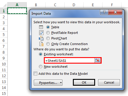
- A dialog box appears requesting how and where to place the data in your worksheet.

- On the dialog box, select any of Table, PivotTable Report, etc.
- Also, select the location for the data. If you choose an existing worksheet, select a cell address. You can leave the default.
- Click Ok and wait for Excel to import the data.
- NOTE: If you want to import data from an existing table in your workbook, select Existing Connection. From the dialog box that appears, select the Tables tab, then the table and click open. Then continue from 11 above.
These are the three (3) basic methods you can use to enter data into Microsoft Excel and other spreadsheet apps.
Formatting data in Excel
Formatting data in Excel involves modifying texts and numbers entered in cells to carry out an analysis. Data entered in Excel may be for presentation, computation, or analysis purposes.
Alignment
Like in Microsoft Word, three types of alignment exist in Microsoft Excel. They include the left, center, and right alignments. Because data is stored in cells, each of these basic alignment types has three modifications: top, middle and bottom.

This means that you can align data in any of the nine different ways: top-left, middle right, bottom center, etc.
When a text is entered, it is aligned at the bottom-left by default, while a number is aligned at the bottom-right by default.
To change the alignment of data in cells, do the following:
- Select the cell or range of cells to be aligned
- On the Home tab, under the Alignment group, select any of the alignment types you want.
- The selected alignment will be applied automatically on the selected cells.
Text and number formatting
You can perform text and number formatting in Excel just as you will do in a Microsoft Word document.
The difference is that instead of selecting text as in word, you will select cells in Excel. The values in cells take the formatting of the cells they reside.
To format the cell content,
- Select the cell or range of cells you want to apply formatting on.
- On the Home tab, under the Fonts group, locate and select the formatting command you want.
- Select your desired command, the content will be automatically formatted. For detail, see Inserting and Formatting Texts.
Formatting cells in Excel
When entering data in excel, other forms of alignment could be used. These types of formatting affect the selected cells and their content. They include merging, shrinking, and wrapping cells.
Merge cells
Merging cells means combining more than one cell. When more than one cell is merged, the combined cells become one. All cells in the group retain the address of the first cell in that group.
If there is content in the cells before the merging, the content of all the cells is lost. However, the content of the first cell in the group is retained. It becomes the content of the merged cell.

To merge cells, do the following:
- Select the group of adjacent cells you want to merge
- On the Home tab, under Alignment group, select Merge & Center.
- The selected cells will be automatically merged.
- Other options exist when you click the dropdown arrow on the Merge & Center command. Experiment with them.
- To unmerge cells, select the merged cell
- On the Home tab, under Alignment group, select Merge & Center. You can click the dropdown arrow button and select Unmerge Cells from the list
Shrink cell content
You can use shrink to fit to reduce the size of the content in a cell. When this is done, the content fits inside the cell without requiring adjustments. However, this is not good when the content is too big for a cell. It can be used only when the content exceeds the size of the cell a little.
To apply shrink to fit, do the following:
- Select the cell or group of cells you want to shrink its content.
- On the Home tab, under Alignment group, select Alignment dialog box launcher.
- A dialog box appears.

- In the dialog box, under the Alignment tab, select the Shrink to fit option button.
- Click Ok when done. The content of the selected cells shrinks to enter the cell.
Wrap cells
Wrapping is used to create a multiline text in a worksheet cell. When the content of a cell is too big, you can either expand the column or wrap the content. If none of this is done, the data in the cell will not show clearly.
To wrap the content of a cell, do the following:
- Select the cell or group of cells you want to wrap their contents
- On the Home tab, under the Alignment group, select Wrap Text.
- The content of selected cells will be automatically wrapped.
- To unwrap the cells, select the wrapped cell and click on the Wrap Text command icon.
Conclusion
We have come to the end of today’s Microsoft Excel tutorial. We were able to look at entering and formatting data in Excel. We began by discussing how you can insert data in a workbook.
We looked at three basic ways of entering data in a worksheet to include: typing, copying, and importing data.
We further discussed how to format data in Excel. We discovered that formatting data in excel implies formatting cells in Excel. This is because data assumes the formatting of the cells they reside. We concluded by looking at different cell formatting options including alignment, merging, and wrapping the content of cells.
These are the basics you need to know before we go into computing and analyzing data in Excel. Particularly, we shall discuss conditional formatting in Excel.
Data entry can sometimes be a big part of using Excel.
With near endless cells, it can be hard for the person inputting data to know where to put what data.
A data entry form can solve this problem and help guide the user to input the correct data in the correct place.
Excel has had VBA user forms for a long time, but they are complicated to set up and not very flexible to change.
In this blog post, we’re going to explore 5 easy ways to create a data entry form for Excel.
Video Tutorial
Excel Tables
We’ve had Excel tables since Excel 2007.
They’re perfect data containers and can be used as a simple data entry form.
Creating a table is easy.
- Select the range of data including the column headings.
- Go to the Insert tab in the ribbon.
- Press the Table button in the Tables section.
We can also use a keyboard shortcut to create a table. The Ctrl + T keyboard shortcut will do the same thing.
Make sure the Create Table dialog box has the My table has headers option checked and press the OK button.
We now have our data inside an Excel table and we can use this to enter new data.
To add new data into our table we can start typing a new entry into the cells directly below the table and the table will absorb the new data.
We can use the Tab key instead of Enter while entering our data. This will cause the active cell cursor to move to the right instead of down so we can add the next value into our record.
When the active cell cursor is in the last cell of the table (lower right cell), pressing the Tab key will create a new empty row in the table ready for the next entry.
This is a perfect and simple data entry form.
Data Entry Form
Excel actually has a hidden data entry form and we can access it by adding the command to the Quick Access Toolbar.
Add the form command to the Quick Access Toolbar.
- Right click anywhere on the quick quick access toolbar.
- Select Customize Quick Access Toolbar from the menu options.
This will open up the Excel option menu on the Quick Access Toolbar tab.
- Select Commands Not in the Ribbon.
- Select Form from the list of available commands. Press F to jump to the commands starting with F.
- Press the Add button to add the command into the quick access toolbar.
- Press the OK button.
We can then open up data entry form for any set of data.
- Select a cell inside the data which we want to create a data entry form with.
- Click on the Form icon in the quick access toolbar area.
This will open up a customized data entry form based on the fields in our data.
Microsoft Forms
If we need a simple data entry form, why not use Microsoft Forms?
This form option will require our Excel workbook to be saved into SharePoint or OneDrive.
The form will be in a browser and not in Excel, but we can link the form to an Excel workbook so that all the data goes into our Excel table.
This is a great option if multiple people or people outside our organization need to input data into the Excel workbook.
We need to create a Form for Excel in either SharePoint or OneDrive. The process is the same for both SharePoint or OneDrive.
- Go to a SharePoint document library or a OneDrive folder where the Excel workbook is going to be saved.
- Click on New and then choose Forms for Excel.
This will prompt us to name the Excel workbook and open up a new browser tab where we can build our form by adding different types of questions.
We first need to create the Form and this will create the table in our Excel workbook where the data will get populated.
Then we can share the form with anyone we want to input data into Excel.
When a user enters data into the form and presses the submit button, that data will automatically show up into our Excel workbook.
Power Apps
Power Apps is a flexible drag and drop formula based app building platform from Microsoft.
We can certainly use it to create a data entry from for our Excel data.
In fact, if we have a table of data set up, Power Apps will create the app for us based on our data. It can’t be any easier than that.
Sign in to the powerapps.microsoft.com service ➜ go to the Create tab in the navigation pane ➜ select Excel Online.
We’ll then be prompted to sign in to our SharePoint or OneDrive account where our Excel file is saved to select the Excel workbook and table with our data.
This will generate us a fully functional three screen data entry app.
- We can search and view all the records in our Excel table in a scroll-able gallery.
- We can view an individual record in our data.
- We can edit an existing record or add new records.
This is all connected to our Excel table, so any changes or additions from the app will show up in Excel.
Power Automate
Power Automate is a cloud based tool for automating task between apps.
But we can use the button trigger to make an automation that captures user input and adds the data into an Excel table.
We’ll need to have our Excel workbook saved in OneDrive or SharePoint and have a table already setup with the fields we want to populate.
To create our Power Automate data entry form.
- Go to flow.microsoft.com and sign in.
- Go to the Create tab.
- Create an Instant flow.
- Give the flow a name.
- Choose the Manually trigger a flow option as the trigger.
- Press the Create button.
This will open up the Power Automate builder and we can build our automation.
- Click on the Manually trigger a flow block to expand the trigger’s options. This is where we’ll find the ability to add input fields.
- Click on the Add an input button. This will give us options to add a few different types of input fields including Text, Yes/No, Files, Email, Number and Dates.
- Rename the field to something descriptive. This will help the user know what type of data to input when they run this automation.
- Click on the three ellipses to the right of each field to change the input options. We’ll be able to Add a drop-down list of option, Add a multi-select list of options, Make the field optional or Delete the field from this menu.
- After we have added all our input fields, we can now add a New step to the automation.
Search for the Excel connector and add the Add a row into a table action. If you’re on an Office 365 business account, use the Excel Online (Business) connectors, otherwise use the Excel Online (OneDrive) connectors.
Now we can set up our Excel Add a row into a table step.
- Navigate to the Excel file and table where we are going to be adding data.
- After selecting the table, the fields in that table will appear listed and we can add the appropriate dynamic content from the Manually trigger a flow trigger step.
Now we can run our Flow from the Power Automate service.
- Go to My flows in the left navigation pane.
- Go to the My flows tab.
- Find the flow in the list of available flows and click on the Run button.
- A side pane will pop up with our inputs and we can enter our data.
- Click Run flow.
We can also run this from our mobile device with the Power Automate apps.
- Go to the Buttons section in the app.
- Press on the flow to run.
- Enter the data inputs in the form.
- Press on the DONE button in the top right.
Whichever way we run the flow, a few seconds later the data will appear in our Excel table.
Conclusions
Whether we require a simple form or something more complex and customize-able, there is a solution for our data entry needs.
We can quickly create something inside our workbook or use an external solution that connects to and loads data into Excel.
We can even create forms that people outside our organization can use to populate our spreadsheets.
Let me know in the comments what is your favourite data entry form option.
About the Author
John is a Microsoft MVP and qualified actuary with over 15 years of experience. He has worked in a variety of industries, including insurance, ad tech, and most recently Power Platform consulting. He is a keen problem solver and has a passion for using technology to make businesses more efficient.
Excel is a preferred option for many people when it comes to processing data. Any calculations can be done with the help of Excel formulas, while Excel macros leave much space for all kinds of automatization.
But not all the data is stored in the form of spreadsheets. There are plenty of systems and tools for data collection and management. Thankfully, Excel is extremely flexible in terms of data importing. This article will explain how you can export data from the most popular sources to Excel.
Importing web data to Excel
Who needs to import data from the web to Excel
It’s not a secret that the internet is made of data. Thanks to the development of broadband networks and wireless technologies, all that data is available at your fingertips at any moment.
But sometimes, you may need to go beyond just reading the information. For example, when you are working on research and want to analyze large amounts of data. In this case, it would be helpful to import web data into specialized software, such as Excel.
How to import data from HTML to Excel
Of course, the simplest way to import data from a website to Excel is to copy-paste it from an HTML page by using a web browser. Sometimes that works pretty well; the simpler, the better. But what if the required data is on hundreds of pages? Or maybe, you don’t need all the information, but only specific fields. In such cases, the simple method will consume an unreasonable amount of time.
Excel has a built-in feature for scraping tables from web pages. To import data from a web source:
- On the Data tab, select New Query > From Other Sources > From Web:
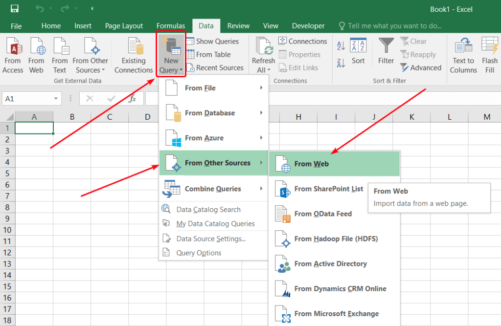
- Enter the web page URL and click OK:

Excel will look for tables on the page.
- In the Navigator window that opens, select the table that you want to import:

Use the Select multiple items checkbox if you want to import several tables. Click Load when you are ready to start the import.
- Excel will insert the imported table into the current worksheet. You can refresh data by clicking the refresh button in the Workbook Queries task pane:

How to automatically import live data into Excel
Data is relevant as long as it’s fresh. If you need to update the information frequently to keep it up-to-date, manual data import will bring nothing but pain.
Thankfully, many websites provide REST API for accessing their data. Sometimes you have to pay for API access, sometimes it’s free. You need to make a request to get the data. The details on making requests can be found in the API reference of the data provider. API responses usually contain data in JSON format. There are free services that allow you to import JSON data to Excel. The best ones will even make API requests for you. Let’s see how you can use Coupler.io for such tasks.
Coupler.io is a data integration solution for importing data into Excel from different apps. You can load records from Shopify, HubSpot, Pipedrive, and many other sources. In addition to Excel, you can use Google Sheets or BigQuery as a destination for your data.
- Sign in to Coupler.io with your Microsoft account.
- Go to Importers and click Add new importer.
- Select JSON as Source, and provide the request URL with your API key (if required):

Refer to the data provider documentation for details on available requests and how you can obtain an API key.
- Specify API call parameters, as described in the API documentation. The only required parameter is HTTP method, which will be ‘GET’ in most cases.
- In Destination, select Microsoft Excel:

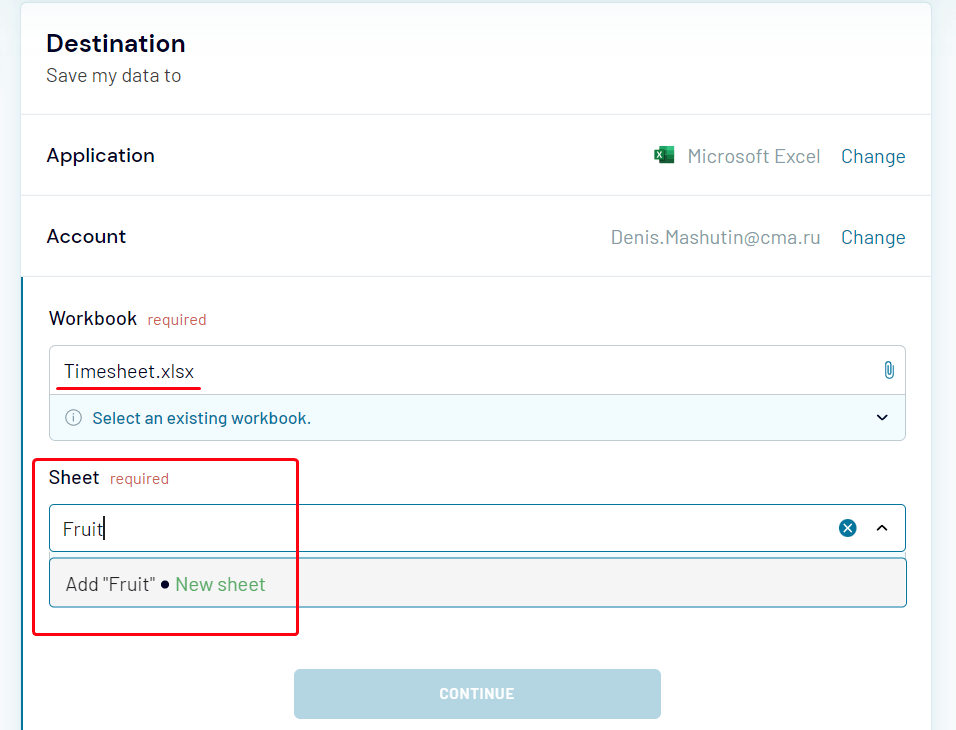
- Connect to your Microsoft Office account, and then select an existing workbook for import. You can specify an existing sheet or create a new one by typing its name:

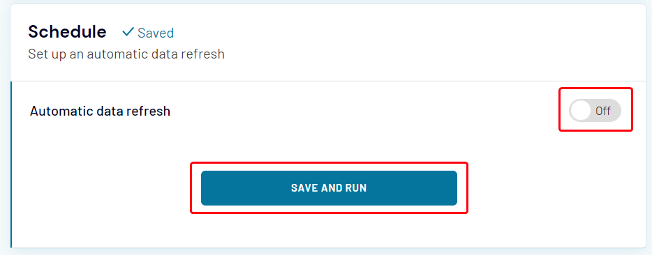
- Toggle the Automatic data refresh switch to set up the schedule for automatic data updates. When you are done with settings, click Save and Run:

Synchronizing the spreadsheets
How to sync data between Excel files
If you want to transfer data from one Excel workbook to another, copy-pasting is a good option. But that will not work if you want to keep the data up-to-date with the other file. There are several ways to sync data between Excel files.
You can use formulas for that. To fill a cell with data from another Excel workbook:
- Make sure that the other workbook is open.
- Select the cell to sync, then click the Formula Bar and type
=.

- Switch to the other workbook, click the cell that you want to import data from, and press Enter.
Excel will switch you back to the first workbook and fill the cell with the synced data. If the content of the cell in the other workbook changes, the synced cell will be updated.
If you see #REF! in the synced cell, it means that the other workbook is not open. Open it to enable data synchronization. Try another method if you are not comfortable with the formula bar.
- In the source file, i.e. the workbook that you want to import data from, select the cell, and then click Copy or press
Ctrl-C:

- Switch to the target workbook, select the cell, and then select Paste > Other Paste Options > Paste Link.
The formula for that cell will be filled with the link to the source cell in the other workbook.
There are many other options for syncing Excel data that you can learn in our guide on linking Excel files.
Besides the standard Excel features, there are online tools that allow you to import data from Excel to Excel, and let you synchronize your data in a more flexible way.
How to import data from Google Sheets to Excel
Google Sheets is almost as powerful as Excel in terms of data processing. But certain very important features are still available only in Excel. If you need these functions, you can transfer your data in several ways.
Import data from Google Sheets to Excel automatically
First of all, try using Coupler.io. It is an online tool that can import data from Google Sheets to Excel.
- Sign in to your Coupler.io account and click Add New in the Importers section.
- Select Google Sheets as Source, click Connect, and sign in to your Google account:
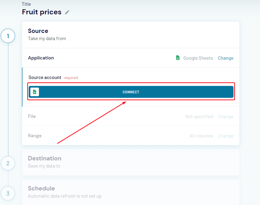
- Select the workbook and the sheet that you would like to export data from:

- Select the range of cells, or skip this step to export all the data.
- In Destination, select Microsoft Excel, click Continue, and then sign in to your Microsoft account.
- Select an existing workbook and the worksheet. If you want to create a new worksheet, just type its name:
- Specify the cell address or keep the default ‘A1’ value.
- Specify the import mode. The default option is ‘Replace’.
- Now you can click Save and Run to start the import immediately.
Or you can toggle Automatic data refresh to configure automatic data updates:
Import data from Google Sheets to Excel as HTML
The second option is to use the built-in data import feature of Excel:
- In your Google spreadsheet, go to File > Share > Publish to web:
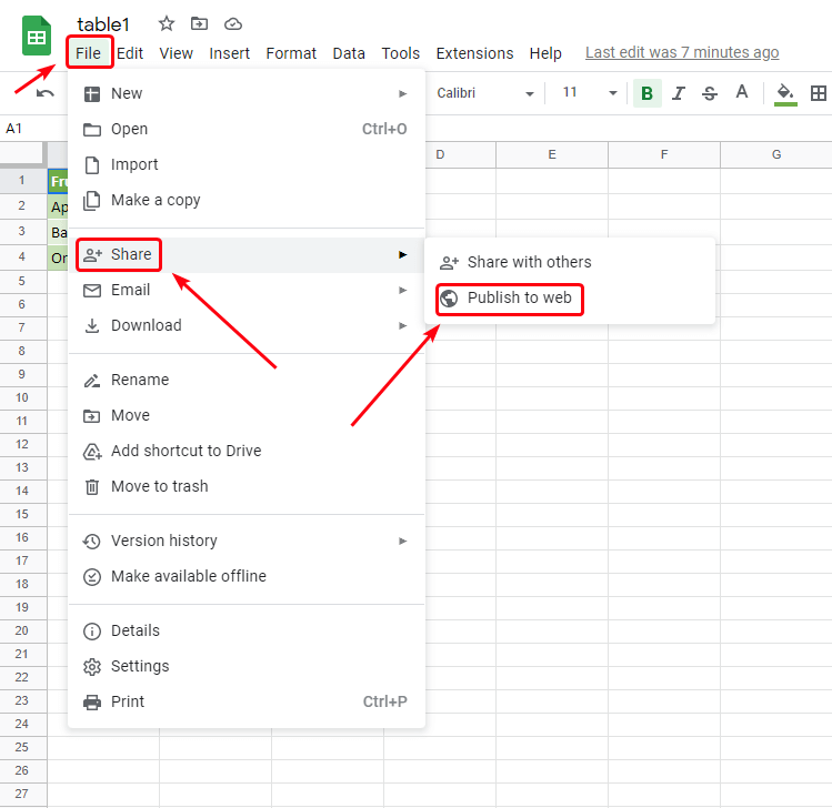
- Select the sheet that contains the table, and specify Comma-separated values (.csv).
If you want the data in Excel to be updated when the Google sheet is changed, select the Automatically republish when changes are made checkbox:

- Press
Ctrl-Cto copy the link. - Go to your Excel workbook and perform the steps described in the section about importing data from HTML above.
If you choose the second option, keep in mind that your data will become accessible by others. If the information is confidential or sensitive, using Coupler.io is preferred.
Importing data from other sources
How to import data from SQL server to Excel
If your data is stored in databases at an SQL server, the simplest way to make it accessible to a wide spectrum of users is to export it to Excel. You can use the native Excel query function.
- In the Data tab, select New Query > From Database > From SQL Server Database:
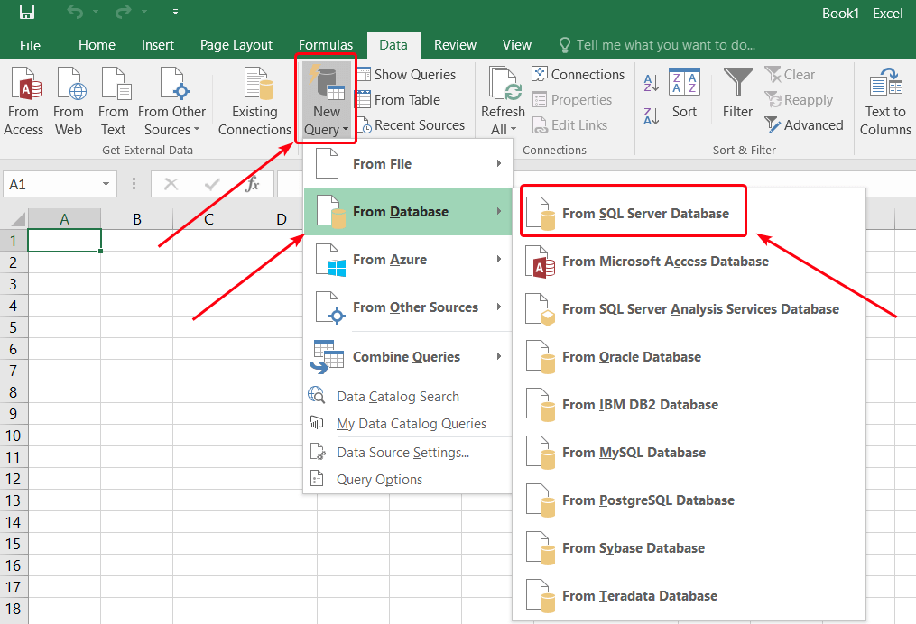
- Specify the name of the server and the database (or you will be able to specify it later):

You can also provide an SQL statement to narrow the range of exported data.
- Choose to use your current window credentials to access the database, or provide the username and the password. Click Connect.
- In the next window, select the database and tables that you want to export.
- Select the name for the new data connection file, and then click Finish.
- In the next window, you can select where to insert the imported data. Select Existing worksheet and provide the cell address, if needed.
The data will be imported and pasted into the worksheet.
If you use SQL Server Management Studio (SSMS), there is a feature for exporting data to various destinations, including Excel spreadsheets.
- In Object Explorer, right-click the database with the source data, and then select Tasks > Export Data.
- In the SQL Server Import and Export Wizard window that opens, click Next.
- Select SQL Server Native Client 11.0 in the Data source drop-down box.
- Select Use Windows Authentication in the Authentication area, and then click Next.
- In the Choose a destination window, specify Microsoft Excel as the destination, browse to the target file in the Excel file path, and select the output file format.
- In the next window, you can choose to write a query for data export. If you want to copy the tables without changes, just click Next.
- The list of tables available for export will be displayed. Select the tables that you want to export. In the Destination column, you can specify the name of the worksheet for each table.
- In the Save and Run Package window, select Run immediately and click Next.
- Make sure that all parameters are correct, and then click Finish.
The selected data will be exported to the Excel workbook. When the wizard finishes all the tasks, click Close.
How to import data from a text file to Excel
The tables can also be stored in plain text. Such files are similar to regular text files with the only exception that commas have a special function there — they separate cells from each other. The format is called CSV — comma-separated values.
Excel can open .csv files directly. The content of such a file will be rendered as a table. If you edit a CSV file in Excel and then try to save it, you will see the following warning:

Click Yes if you want to continue using this file as CSV in the future. If you click No, the Save as dialogue will be opened, where you will be able to select the format and the destination for the file.
There are other delimiters that can be used to store tables in text format: tabs, pipes (‘|’), spaces, semicolons, etc. To open such files with Excel, instead of trying to open them directly, use the Power Query function.
- Go to Data > New Query > From File > From Text.
- Select the text file and click Import.
- The Query Editor window will open. Make sure that the table looks good and click Close & Load:

The imported table will be inserted into your current worksheet.
How to import data to Excel from PDF
If your tables are in PDF, but you want them in Excel, you can try to import them.
- Go to the Data tab, and then select New Query > From File > From PDF.
- Select the tables that you want to import in the Navigator window, and then click Load.
The tables will be extracted from PDF and pasted into your Excel workbook. If you don’t have the From PDF option on the menu, you can use the following workaround to import data from PDF into Excel:
- Copy the table text in the PDF file by selecting it and pressing
Ctrl-C. - Open Microsoft Word and press
Ctrl-V. - Check if Word managed to render the text data correctly:
- Press
Ctrl-Ato select everything. - On the Home tab, click the table menu, and then select All borders:
- Press
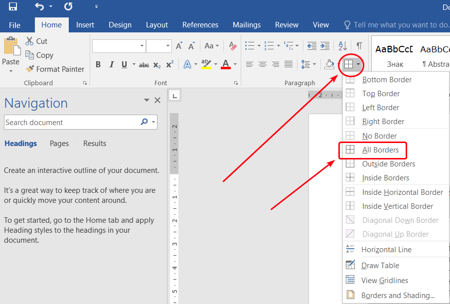
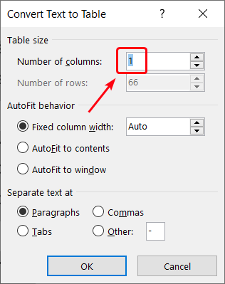
- If the table looks good, proceed to the final step. Otherwise, go to the Insert tab, and then select Table > Convert Text to Table:

- Specify the number of columns in the original table, and then click OK:
- Copy the entire table, go to Excel, and press
Ctrl-V.
The table will be inserted into the current worksheet. If you opt for this workaround, no automatic data synchronization will be available.
Discover many other sources for importing data to Excel
Excel provides you with many powerful features for data processing. You can bring virtually any data to Excel by importing it from various sources. If you didn’t find a good solution in this article, discover other Microsoft Excel integrations to pick what fits your needs best.
-

Lead Analytics Engineer at Railsware and Coupler.io. I make data accessible and useful for everyone in a team. During the last 7 years, I built dashboards, analyzed user journeys, and even caught criminals 🕵🏿♀️ Besides data, I also like doing yoga, cooking, and hiking 🤗

Back to Blog
Focus on your business
goals while we take care of your data!
Try Coupler.io