
Enter data manually in worksheet cells
Excel for Microsoft 365 Excel 2021 Excel 2019 Excel 2016 Excel 2013 Excel 2010 Excel 2007 More…Less
You have several options when you want to enter data manually in Excel. You can enter data in one cell, in several cells at the same time, or on more than one worksheet at once. The data that you enter can be numbers, text, dates, or times. You can format the data in a variety of ways. And, there are several settings that you can adjust to make data entry easier for you.
This topic does not explain how to use a data form to enter data in worksheet. For more information about working with data forms, see Add, edit, find, and delete rows by using a data form.
Important: If you can’t enter or edit data in a worksheet, it might have been protected by you or someone else to prevent data from being changed accidentally. On a protected worksheet, you can select cells to view the data, but you won’t be able to type information in cells that are locked. In most cases, you should not remove the protection from a worksheet unless you have permission to do so from the person who created it. To unprotect a worksheet, click Unprotect Sheet in the Changes group on the Review tab. If a password was set when the worksheet protection was applied, you must first type that password to unprotect the worksheet.
-
On the worksheet, click a cell.
-
Type the numbers or text that you want to enter, and then press ENTER or TAB.
To enter data on a new line within a cell, enter a line break by pressing ALT+ENTER.
-
On the File tab, click Options.
In Excel 2007 only: Click the Microsoft Office Button
 , and then click Excel Options.
 -
Click Advanced, and then under Editing options, select the Automatically insert a decimal point check box.
-
In the Places box, enter a positive number for digits to the right of the decimal point or a negative number for digits to the left of the decimal point.
For example, if you enter 3 in the Places box and then type 2834 in a cell, the value will appear as 2.834. If you enter -3 in the Places box and then type 283, the value will be 283000.
-
On the worksheet, click a cell, and then enter the number that you want.
Data that you typed in cells before selecting the Fixed decimal option is not affected.
To temporarily override the Fixed decimal option, type a decimal point when you enter the number.
 , and then click Excel Options.
-
On the worksheet, click a cell.
-
Type a date or time as follows:
-
To enter a date, use a slash mark or a hyphen to separate the parts of a date; for example, type 9/5/2002 or 5-Sep-2002.
-
To enter a time that is based on the 12-hour clock, enter the time followed by a space, and then type a or p after the time; for example, 9:00 p. Otherwise, Excel enters the time as AM.
To enter the current date and time, press Ctrl+Shift+; (semicolon).
-
-
To enter a date or time that stays current when you reopen a worksheet, you can use the TODAY and NOW functions.
-
When you enter a date or a time in a cell, it appears either in the default date or time format for your computer or in the format that was applied to the cell before you entered the date or time. The default date or time format is based on the date and time settings in the Regional and Language Options dialog box (Control Panel, Clock, Language, and Region). If these settings on your computer have been changed, the dates and times in your workbooks that have not been formatted by using the Format Cells command are displayed according to those settings.
-
To apply the default date or time format, click the cell that contains the date or time value, and then press Ctrl+Shift+# or Ctrl+Shift+@.
-
Select the cells into which you want to enter the same data. The cells do not have to be adjacent.
-
In the active cell, type the data, and then press Ctrl+Enter.
You can also enter the same data into several cells by using the fill handle
to automatically fill data in worksheet cells.For more information, see the article Fill data automatically in worksheet cells.
 to automatically fill data in worksheet cells.
By making multiple worksheets active at the same time, you can enter new data or change existing data on one of the worksheets, and the changes are applied to the same cells on all the selected worksheets.
-
Click the tab of the first worksheet that contains the data that you want to edit. Then hold down Ctrl while you click the tabs of other worksheets in which you want to synchronize the data.
Note: If you don’t see the tab of the worksheet that you want, click the tab scrolling buttons to find the worksheet, and then click its tab. If you still can’t find the worksheet tabs that you want, you might have to maximize the document window.
-
On the active worksheet, select the cell or range in which you want to edit existing or enter new data.
-
In the active cell, type new data or edit the existing data, and then press Enter or Tab to move the selection to the next cell.
The changes are applied to all the worksheets that you selected.
-
Repeat the previous step until you have completed entering or editing data.

-
To cancel a selection of multiple worksheets, click any unselected worksheet. If an unselected worksheet is not visible, you can right-click the tab of a selected worksheet, and then click Ungroup Sheets.
-
When you enter or edit data, the changes affect all the selected worksheets and can inadvertently replace data that you didn’t mean to change. To help avoid this, you can view all the worksheets at the same time to identify potential data conflicts.
-
On the View tab, in the Window group, click New Window.
-
Switch to the new window, and then click a worksheet that you want to view.
-
Repeat steps 1 and 2 for each worksheet that you want to view.
-
On the View tab, in the Window group, click Arrange All, and then click the option that you want.
-
To view worksheets in the active workbook only, in the Arrange Windows dialog box, select the Windows of active workbook check box.
-
There are several settings in Excel that you can change to help make manual data entry easier. Some changes affect all workbooks, some affect the whole worksheet, and some affect only the cells that you specify.
Change the direction for the Enter key
When you press Tab to enter data in several cells in a row and then press Enter at the end of that row, by default, the selection moves to the start of the next row.
Pressing Enter moves the selection down one cell, and pressing Tab moves the selection one cell to the right. You cannot change the direction of the move for the Tab key, but you can specify a different direction for the Enter key. Changing this setting affects the whole worksheet, any other open worksheets, any other open workbooks, and all new workbooks.
-
On the File tab, click Options.
In Excel 2007 only: Click the Microsoft Office Button
, and then click Excel Options. -
In the Advanced category, under Editing options, select the After pressing Enter, move selection check box, and then click the direction that you want in the Direction box.
Change the width of a column
At times, a cell might display #####. This can occur when the cell contains a number or a date and the width of its column cannot display all the characters that its format requires. For example, suppose a cell with the Date format «mm/dd/yyyy» contains 12/31/2015. However, the column is only wide enough to display six characters. The cell will display #####. To see the entire contents of the cell with its current format, you must increase the width of the column.
-
Click the cell for which you want to change the column width.
-
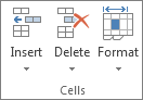
On the Home tab, in the Cells group, click Format.
-
Under Cell Size, do one of the following:
-
To fit all text in the cell, click AutoFit Column Width.
-
To specify a larger column width, click Column Width, and then type the width that you want in the Column width box.
-
Note: As an alternative to increasing the width of a column, you can change the format of that column or even an individual cell. For example, you could change the date format so that a date is displayed as only the month and day («mm/dd» format), such as 12/31, or represent a number in a Scientific (exponential) format, such as 4E+08.
Wrap text in a cell
You can display multiple lines of text inside a cell by wrapping the text. Wrapping text in a cell does not affect other cells.
-
Click the cell in which you want to wrap the text.
-
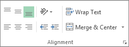
On the Home tab, in the Alignment group, click Wrap Text.
Note: If the text is a long word, the characters won’t wrap (the word won’t be split); instead, you can widen the column or decrease the font size to see all the text. If all the text is not visible after you wrap the text, you might have to adjust the height of the row. On the Home tab, in the Cells group, click Format, and then under Cell Size click AutoFit Row.
For more information on wrapping text, see the article Wrap text in a cell.
Change the format of a number
In Excel, the format of a cell is separate from the data that is stored in the cell. This display difference can have a significant effect when the data is numeric. For example, when a number that you enter is rounded, usually only the displayed number is rounded. Calculations use the actual number that is stored in the cell, not the formatted number that is displayed. Hence, calculations might appear inaccurate because of rounding in one or more cells.
After you type numbers in a cell, you can change the format in which they are displayed.
-
Click the cell that contains the numbers that you want to format.
-
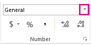
On the Home tab, in the Number group, click the arrow next to the Number Format box, and then click the format that you want.
To select a number format from the list of available formats, click More Number Formats, and then click the format that you want to use in the Category list.
Format a number as text
For numbers that should not be calculated in Excel, such as phone numbers, you can format them as text by applying the Text format to empty cells before typing the numbers.
-
Select an empty cell.
-
On the Home tab, in the Number group, click the arrow next to the Number Format box, and then click Text.
-
Type the numbers that you want in the formatted cell.
Numbers that you entered before you applied the Text format to the cells must be entered again in the formatted cells. To quickly reenter numbers as text, select each cell, press F2, and then press Enter.
Need more help?
You can always ask an expert in the Excel Tech Community or get support in the Answers community.
Need more help?
Once you know how to enter data into an Excel worksheet you will be setting up tables of data in no time.
When you haven’t been shown how to enter data it can be a little tricky, so follow the steps below to learn the tips and hacks to entering your data easily into your worksheet.
Entering data into an Excel worksheet
You can enter either values (numbers and dates) or labels (text) into any cell within the worksheet.
1. Move the cell pointer to the required cell and then type the data. While you type the data you will notice that it appears both in the worksheet (in the example below, the text appears in cell A1) and in the Formula Bar.
2. Press ENTER to enter the information into the cell. Your cell pointer will move down to the cell below.
Tip: If you press the ESC key instead of ENTER the data will not be entered into the cell.
Deleting and replacing data
- To delete data select the cell containing the data and then press DELETE.
- To replace data just type directly over the top of the existing cell contents. The new data will replace the old.
Using Undo and Redo
There will be times when you enter data only to realise you have made a bit of a mess of things.
Most times you want to back-back to where you were before the mistake was made. If this happens you can click the fabulous “Undo” button which will undo the last thing you did.
You can actually keep clicking it until you get back to a point where you feel in control again.
And if you go one step to far back, you can click the Redo button to go forward a step again. These buttons are fabulous and you use them a lot.
Overlapping data
If you enter data that will not fit the column width it will overlap into the next column. In the example below the text ‘Travel Expenses’ is entered into cell A1, however it looks as though the text is included in cells B1. With cell A1 selected we can see in the Formula bar that both words are indeed in A1.
If you are not using the column into which the text is overlapping you may leave the text as it is. However, as soon as you place text into a cell that has been overlapped it will look as if your text has been lost. In the example below, the text ‘Amount ex GST’ has been entered into cell C3. However the content of cell D3 is hiding part of the content is C3.
By selecting C3 the entire cell’s content can be seen in the Formula Bar. In order to view the entire contents of cell C3 the width of column C needs to be adjusted.
Working with columns
The standard column width for Excel is 8.43 character spaces. You can change the column width by dragging with your mouse on the column headers, or by double clicking between two column headers.
Tip: If multiple columns require the same width, select the columns and widen one of them with the mouse. The rest will be adjusted to the same width.
Adjusting the column width
To use your mouse to adjust the column width:
1. Move your mouse pointer over the column’s right edge in the column header area. Your mouse pointer should change to a double-headed arrow.
2. Click and drag to the right to expand, or to the left to shrink the column width to the size you require.
You will now be able to see your entire text. Continue dragging until all columns are the width you require.
Tips:
To quickly adjust the column width to fit the widest entry, move your mouse pointer over the lines between the column headers. When the pointer becomes a double-headed arrow double-click.
Use the same method for adjusting the height of any row. Just move the mouse pointer over the line separating the rows. When the pointer becomes a double-headed arrow, drag or double-click to adjust the row height, or double-click to set the height to fit the tallest entry.
By the way, row heights will automatically alter if the font size of data is altered.
Extra info: to set a column width to a precise measurement on the Home tab in the Cells group select Format and then select Column Width. Type the desired width in the Column Width box and then click OK to accept the new column width.
What do hash signs mean in Excel?
If you ever see a cell containing ######## (hash signs) it means the column isn’t wide enough to display the content. Just extend the width and the content will become visible.
Making changes to the data
Once you have entered data into your worksheet, you can edit the data in a number of ways.
- Select the cell and then click in the Formula bar. A flashing insertion point will be placed into the bar. Use the arrow keys on the keyboard to move the insertion point. Make the changes you require and then press ENTER.
- You may also type directly over the data in the cell with new data and then press ENTER. The new data will replace the old.
- Double clicking a cell or pressing F2 allows you to edit the contents of the cell directly on the worksheet. Make the changes and then press ENTER to update the cell.
AutoComplete
AutoComplete is the ability for Excel to automatically complete an entry for you.
For example, if you have typed text in the cells above as soon as you start typing a letter or two in a cell below, Excel will check the list above for a matching entry and complete the entry for you.
This can be very useful when you need to make the same entry several times.
To accept the entry press ENTER. To reject the displayed entry and type something different either ignore the entry and type right over it or press DELETE.
Was this blog helpful? Let us know in the Comments below.
Instructions
Entering data into an Excel worksheet
- Move the cell pointer to the required cell and then type the data.
- Press ENTER to enter the information into the cell. Your cell pointer will move down to the cell below.
Deleting and replacing data
To Delete: Select the cell containing the data and then press DELETE.
To replace data: Type directly over the top of the existing cell contents. The new data will replace the old.
Using Undo and Redo
If you make a mistake, you can use the Undo button on the top right of the Excel spreadsheet to undo the last thing you did. You can keep clicking it to go back multiple steps.
If you Undo something you didn’t want undone, you can use the Redo button to the right of the Undo button to go forward a step again.
Overlapping data
If you enter data that will not fit the column width it will overlap into the next column. Adjust the width of the columns in order to view the entire contents.
Working with columns
Adjusting the column width
- Move your mouse pointer over the column’s right edge in the column header area. Your mouse pointer should change to a double-headed arrow.
- Click and drag to the right to expand, or to the left to shrink the column width to the size you require.
- You will now be able to see your entire text. Continue dragging until all columns are the width you require.
Making changes to the data
- Select the cell and then click in the Formula bar. A flashing insertion point will be placed into the bar. Use the arrow keys on the keyboard to move the insertion point. Make the changes you require and then press ENTER.
- You may also type directly over the data in the cell with new data and then press ENTER. The new data will replace the old.
- Double clicking a cell or pressing F2 allows you to edit the contents of the cell directly on the worksheet. Make the changes and then press ENTER to update the cell.
AutoComplete
Sometimes when you are typing in a cell, Excel will automatically complete the entry for you. To accept the entry press ENTER. To reject the displayed entry and type something different either ignore the entry and type right over it or press DELETE.
Notes
Note: While you type the data you will notice that it appears both in the worksheet cell and in the Formula Bar.
Tip: If you press the ESC key instead of ENTER when typing data into a cell the data will not be entered into the cell.
Tips: To quickly adjust the column width to fit the widest entry, move your mouse pointer over the lines between the column headers. When the pointer becomes a double-headed arrow double-click.
Extra info: to set a column width to a precise measurement on the Home tab in the Cells group select Format and then select Column Width. Type the desired width in the Column Width box and then click OK to accept the new column width.
Note: If you ever see a cell containing ######## (hash signs) it means the column isn’t wide enough to display the content. Just extend the width and the content will become visible.
Entering Data and Moving in Excel Worksheet
Entering Data and Moving in Excel Worksheet is very easy and you find that it is the time saver for data entry. You can enter any numbers, text, dates in Excel and you can format as per your requirement.
Entering Data
Active Cell is the place where we enter the data. When we open a new Excel Workbook, by default it activates A1 (top-left corner of a Worksheet) position of a Worksheet and we can start entering the data.
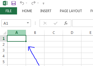
We can observe the A1 is activate and you can see the Address of the active Cell in the Address bar (rounded with red circle), you can also observe the sample text in A1.

We can also activate a Cell and enter the data in Formula bar.

So, we can activate any Cell and enter the data as per our requirement, below is the example data entered in a worksheet.

Editing Data
We can simply select any Cell and enter new data to edit the existing data in a Cell.
If you want to edit a particular part of existing data, then you need to activate (by pressing F2 or double clicking with the mouse), then goto the particular position and change the data. The other method is using Formula bar, it will give more flexibility to enter the data. To do this, select a Cell and go to Formula bar then start editing or entering the data.
Useful Shortcut Keys to Move in the Worksheet
The below short-cut keys helps us to move in a Worksheet:
| To move | Press this key |
|---|---|
| One cell right | Right Arrow Or Tab |
| One cell left | Left Arrow Or Shift + Tab |
| One cell up | Up Arrow Or Shift + Enter |
| One cell down | Down Arrow Or Enter |
| To top of worksheet (cell A1) | Ctr + Home |
| To last cell containing data | Ctr + End |
| To end of data in a column | Ctr + Down Arrow |
| To beginning of data in a column | Ctr + Up Arrow |
| To end of data in a row | Ctr + Right Arrow |
| To beginning of data in a row | Ctr + Left Arrow |
| Towards Right | Ctr + Left Arrow |
You can also use, Go To Command (You can enable the Go To Command by pressing the Ctr+G. For example, if you want to Activate A22, enter A22 in the Reference space of the Go To Command and then press OK button.

You can also use Address bar to move around the Worksheet and Activate a particular Cell. For example, if you want to Activate C12, enter C12 in the Adress Bar and then press Enter Key.

A Powerful & Multi-purpose Templates for project management. Now seamlessly manage your projects, tasks, meetings, presentations, teams, customers, stakeholders and time. This page describes all the amazing new features and options that come with our premium templates.
Save Up to 85% LIMITED TIME OFFER

All-in-One Pack
120+ Project Management Templates
Essential Pack
50+ Project Management Templates
Excel Pack
50+ Excel PM Templates
PowerPoint Pack
50+ Excel PM Templates
MS Word Pack
25+ Word PM Templates
Ultimate Project Management Template
Ultimate Resource Management Template
Project Portfolio Management Templates
Related Posts
- Entering Data
- Editing Data
- Useful Shortcut Keys to Move in the Worksheet
VBA Reference
Effortlessly
Manage Your Projects
120+ Project Management Templates
Seamlessly manage your projects with our powerful & multi-purpose templates for project management.
120+ PM Templates Includes:
Effectively Manage Your
Projects and Resources
ANALYSISTABS.COM provides free and premium project management tools, templates and dashboards for effectively managing the projects and analyzing the data.
We’re a crew of professionals expertise in Excel VBA, Business Analysis, Project Management. We’re Sharing our map to Project success with innovative tools, templates, tutorials and tips.
Project Management
Excel VBA
Download Free Excel 2007, 2010, 2013 Add-in for Creating Innovative Dashboards, Tools for Data Mining, Analysis, Visualization. Learn VBA for MS Excel, Word, PowerPoint, Access, Outlook to develop applications for retail, insurance, banking, finance, telecom, healthcare domains.
Page load link
Go to Top
Watch the Video on Using Data Entry Forms in Excel
Below is a detailed written tutorial about Excel Data Entry form in case you prefer reading over watching a video.
Excel has many useful features when it comes to data entry.
And one such feature is the Data Entry Form.
In this tutorial, I will show you what are data entry forms and how to create and use them in Excel.
Why Do You Need to Know About Data Entry Forms?
Maybe you don’t!
But if data entry is a part of your daily work, I recommend you check out this feature and see how it can help you save time (and make you more efficient).
There are two common issues that I have faced (and seen people face) when it comes to data entry in Excel:
- It’s time-consuming. You need to enter the data in one cell, then go to the next cell and enter the data for it. Sometimes, you need to scroll up and see which column it is and what data needs to be entered. Or scroll to the right and then come back to the beginning in case there are many columns.
- It’s error-prone. If you have a huge data set which needs 40 entries, there is a possibility you may end up entering something that was not intended for that cell.
A data entry form can help by making the process faster and less error-prone.
Before I show you how to create a data entry form in Excel, let me quickly show you what it does.
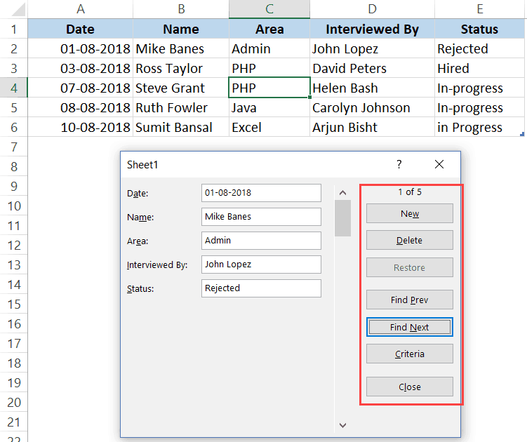
Below is a data set that is typically maintained by the hiring team in an organization.
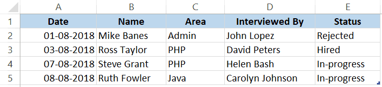
Every time a user has to add a new record, he/she will have to select the cell in the next empty row and then go cell by cell to make the entry for each column.
While this is a perfectly fine way of doing it, a more efficient way would be to use a Data Entry Form in Excel.
Below is a data entry form that you can use to make entries to this data set.
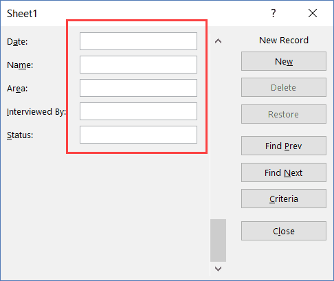
The highlighted fields are where you would enter the data. Once done, hit the Enter key to make the data a part of the table and move on to the next entry.
Below is a demo of how it works:
As you can see, this is easier than regular data entry as it has everything in a single dialog box.
Data Entry Form in Excel
Using a data entry form in Excel needs a little pre-work.
You would notice that there is no option to use a data entry form in Excel (not in any tab in the ribbon).
To use it, you will have to first add it to the Quick Access Toolbar (or the ribbon).
Adding Data Entry Form Option To Quick Access Toolbar
Below are the steps to add the data entry form option to the Quick Access Toolbar:
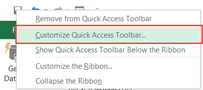
- Right-click on any of the existing icons in the Quick Access Toolbar.
- Click on ‘Customize Quick Access Toolbar’.

- In the ‘Excel Options’ dialog box that opens, select the ‘All Commands’ option from the drop-down.

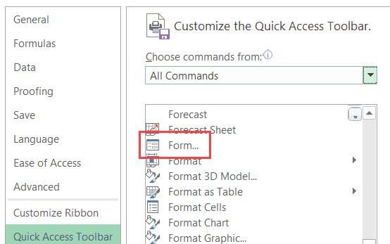
- Scroll down the list of commands and select ‘Form’.

- Click on the ‘Add’ button.

- Click OK.


The above steps would add the Form icon to the Quick Access Toolbar (as shown below).
![]()
Once you have it in QAT, you can click any cell in your dataset (in which you want to make the entry) and click on the Form icon.
Note: For Data Entry Form to work, your data should be in an Excel Table. If it isn’t already, you’ll have to convert it into an Excel Table (keyboard shortcut – Control + T).
Parts of the Data Entry Form
A Data Entry Form in Excel has many different buttons (as you can see below).
Here is a brief description of what each button is about:
- New: This will clear any existing data in the form and allows you to create a new record.
- Delete: This will allow you to delete an existing record. For example, if I hit the Delete key in the above example, it will delete the record for Mike Banes.
- Restore: If you’re editing an existing entry, you can restore the previous data in the form (if you haven’t clicked New or hit Enter).
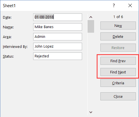
- Find Prev: This will find the previous entry.
- Find Next: This will find the next entry.
- Criteria: This allows you to find specific records. For example, if I am looking for all the records, where the candidate was Hired, I need to click the Criteria button, enter ‘Hired’ in the Status field and then use the find buttons. Example of this is covered later in this tutorial.
- Close: This will close the form.
- Scroll Bar: You can use the scroll bar to go through the records.
Now let’s go through all the things you can do with a Data Entry form in Excel.
Note that you need to convert your data into an Excel Table and select any cell in the table to be able to open the Data Entry form dialog box.
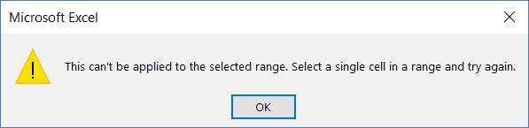
If you haven’t selected a cell in the Excel Table, it will show a prompt as shown below:
Creating a New Entry
Below are the steps to create a new entry using the Data Entry Form in Excel:
- Select any cell in the Excel Table.
- Click on the Form icon in the Quick Access Toolbar.

- Enter the data in the form fields.
- Hit the Enter key (or click the New button) to enter the record in the table and get a blank form for next record.
Navigating Through Existing Records
One of the benefits of using Data Entry Form is that you can easily navigate and edit the records without ever leaving the dialog box.
This can be especially useful if you have a dataset with many columns. This can save you a lot of scrolling and the process of going back and forth.
Below are the steps to navigate and edit the records using a data entry form:
- Select any cell in the Excel Table.
- Click on the Form icon in the Quick Access Toolbar.
- To go to the next entry, click on the ‘Find Next’ button and to go to the previous entry, click the ‘Find Prev’ button.

- To edit an entry, simply make the change and hit enter. In case you want to revert to the original entry (if you haven’t hit the enter key), click the ‘Restore’ button.
You can also use the scroll bar to navigate through entries one-by-one.
The above snapshot shows basic navigation where you are going through all the records one after the other.
But you can also quickly navigate through all the records based on criteria.
For example, if you want to go through all the entries where the status is ‘In-progress’, you can do that using the below steps:
Criteria is a very useful feature when you have a huge dataset, and you want to quickly go through those records that meet a given set of criteria.
Note that you can use multiple criteria fields to navigate through the data.
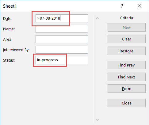
For example, if you want to go through all the ‘In-progress’ records after 07-08-2018, you can use ‘>07-08-2018’ in the criteria for ‘Date’ field and ‘In-progress’ as the value in the status field. Now when you navigate using Find Prev/Find Next buttons, it will only show records after 07-08-2018 where the status is In-progress.
You can also use wildcard characters in criteria.
For example, if you have been inconsistent in entering the data and have used variations of a word (such as In progress, in-progress, in progress, and inprogress), then you need to use wildcard characters to get these records.
Below are the steps to do this:
- Select any cell in the Excel table.
- Click on the Form icon in the Quick Access Toolbar.
- Click the Criteria button.
- In the Status field, enter *progress
- Use the Find Prev/Find Next buttons to navigate through the entries where the status is In-Progress.

This works as an asterisk (*) is a wildcard character that can represent any number of characters in Excel. So if the status contains the ‘progress’, it will be picked up by Find Prev/Find Next buttons no matter what is before it).
Deleting a Record
You can delete records from the Data Entry form itself.
This can be useful when you want to find a specific type of records and delete these.
Below are the steps to delete a record using Data Entry Form:
- Select any cell in the Excel table.
- Click on the Form icon in the Quick Access Toolbar.
- Navigate to the record you want to delete
- Click the Delete button.

While you may feel that this all looks like a lot of work just to enter and navigate through records, it saves a lot of time if you’re working with lots of data and have to do data entry quite often.
Restricting Data Entry Based on Rules
You can use data validation in cells to make sure the data entered conforms to a few rules.
For example, if you want to make sure that the date column only accepts a date during data entry, you can create a data validation rule to only allow dates.
If a user enters a data that is not a date, it will not be allowed and the user will be shown an error.
Here is how to create these rules when doing data entry:
- Select the cells (or even the entire column) where you want to create a data validation rule. In this example, I have selected column A.
- Click the Data tab.

- Click the Data Validation option.

- In the ‘Data Validation’ dialog box, within the ‘Settings’ tab, select ‘Date’ from the ‘Allow’ drop down.

- Specify the start and the end date. Entries within this date range would be valid and rest all would be denied.
- Click OK.


Now, if you use the data entry form to enter data in the Date column, and if it isn’t a date, then it will not be allowed.
You will see a message as shown below:
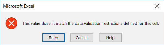
Similarly, you can use data validation with data entry forms to make sure users don’t end up entering the wrong data. Some examples where you can use this is numbers, text length, dates, etc.
Here are a few important things to know about Excel Data Entry Form:
- You can use wildcard characters while navigating through the records (through criteria option).
- You need to have an Excel table to be able to use the Data Entry Form. Also, you need to have a cell selected in it to use the form. There is one exception to this though. If you have a named range with the name ‘Database’, then the Excel Form will also refer to this named range, even if you have an Excel table.
- The field width in the Data Entry form is dependent on the column width of the data. If your column width is too narrow, the same would be reflected in the form.
- You can also insert bullet points in the data entry form. To do this, use the keyboard shortcut ALT + 7 or ALT + 9 from your numeric keypad. Here is a video about bullet points.
You May Also Like the Following Excel Tutorials:
- 100+ Excel Interview Questions.
- Drop Down Lists in Excel.
- Find and Remove Duplicates in Excel.
- Excel Text to Columns.
Entering Data
The first step in creating a useful worksheet is entering data. By entering data, you are inputting the information that you want Excel to display, calculate, and store. Data can be entered into a cell or a range of cells. You can even set up a sequence of data and let Excel fill in the remainder of the sequence based on your first few entries.
Looking for Excel training in Los Angeles?
Identifying Types of Data
Excel worksheets contain four types of data: text, values, dates, and formulas. Examples of each are found in Table 1-2.
| Text | Value | Date | Formula |
| Supplies | 852.34 | 12/3/02 | =C3+D3+E3 |
| 12 Dozen | 42980.00254 | Jan 3, 2001 | =245*C3 |
Table 1-2 : Examples of Data Types
Text data is alphanumeric and cannot be used in most formulas. Values are numerals only. Although a date may seem to be text, as soon as you enter what Excel recognizes as a date, it is formatted and stored using a decimal date format. As a result, dates can be used in complex functions.
Formulas are made up of values and operators. Because formulas contain references to worksheet cells and ranges, they depend on other elements of the worksheet. For instance, if a formula includes a reference to cell C3 and you change the value that is located in C3, the result of the formula will change accordingly.
Entering Text Data into a Cell
A single cell can hold up to 32,000 alphanumeric characters. If the cell is not wide enough and if the cell to the right contains data, some characters may not be visible. Excel hasn’t lost this data; it just doesn’t show it.
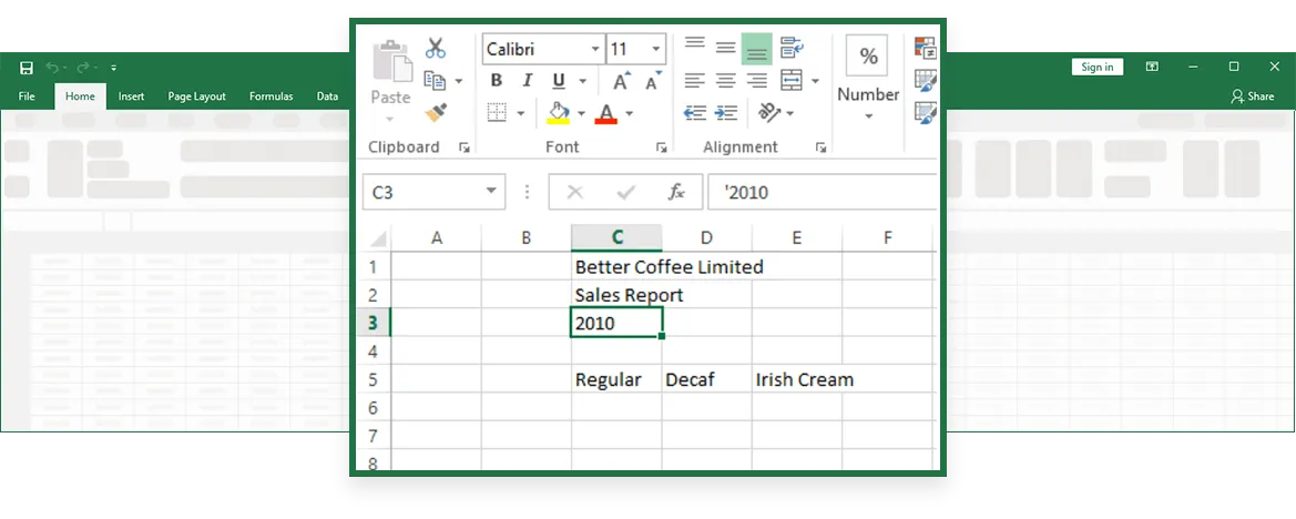
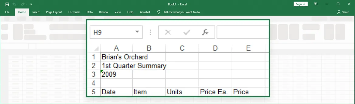
On occasion, you may need to enter a number as text. For example, you may want to exclude a number from a summed column. If you type an apostrophe (’) before the number, for example ‘2013, Excel accepts it as text and aligns it on the left, as illustrated in Figure 1-9. All other numbers are right-aligned by default. The apostrophe does not show up in the worksheet cell, but you can see it in the Formula bar. You don’t need to type the apostrophe when a phrase begins with a number as long as it includes text characters, for example, 1st Quarter Summary.
Note Excel 2013 will produce an error at this point de-noted by a green arrow in the top left corner of the cell (This error indicates inconsistent data i.e. number formatted as text). A yellow diamond with an ! in the middle will also appear with options to correct this error.
When you enter functional data into your worksheet (that is a calculation or part thereof; e.g. the equals sign), three buttons appear in the Formula bar to the right of the Name box, shown in Figure 1‑6. Use the Cancel button if you decide not to continue to enter the data into the cell and the Enter button to accept the entry. The Edit Formula button is only operable when the cell contains a formula.
Method
To enter text data into a cell:
- Select the cell.
- Type the information in the cell.
- Click the Enter button.
or - Press Enter to enter the data and move down one cell.
or - Select another cell.
To cancel data before it is entered:
- Click the Cancel button.
or - Press Esc
Exercise
In the following exercise, you will enter text data into cells.
- Select cell A1.
- Type Brian’s Orchard.
- Click the Enter button. [Brian’s Orchard appears in A1, and appears to flow into the next column. A1 is still the active cell].
- Select cell A2.
- Type 1st Quarter Summary.
- Click cell A3. [1st Quarter Summary appears in cell A2 and cell A3 is the active cell].
- Type 2013.
- Click the Cancel button. [The entry is canceled].
- Type ‘2013.
- Press Enter. [2013 appears in cell A3 as text and A4 is the active cell].
- Using the worksheet below, enter the headings for cells A5, B5, C5, D5, and E5.
Entering Values
You enter values into the worksheet the same way you enter text. However, it’s important to note that values can contain only the following characters:
1 2 3 4 5 6 7 8 9 0 + - ( ) , / $ % . E e
Method
To enter values in a cell:
- Select the cell.
- Type the value in the cell.
- Click the Enter button.
or - Press Enter to enter the value and move down one cell.
or - Select another cell.
Exercise
In the following exercise, you will enter values into cells.
- Select cell C6.
- Type 65. [The range A1 to D5 is selected].
- Click the Enter button. [65 appears in cell C6].
- Select cell C7.
- Type 35. [35 appears in cell C7].
- Select cell C8.
- Type 20.
- Press Enter. [20 appears in cell C8].
- In cell D6, enter 0.59.
- In cell D7, enter 1.12.
- In cell D8, enter -0.25.
Entering Data into a Range
Selecting an entire worksheet is useful when you want to make changes on a global scale. For instance, you might want to change the size of the font in every cell in the worksheet. Once you select the entire worksheet using the Select All button, illustrated in Figure 1-4, you can do this in a single step.
Method
In the following exercise, you will enter data into a range.
- Select the desired range.
- Type the information into the first cell.
- Press Enter to move to the next cell.
- Type the appropriate information.
- Repeat steps 3 and 4 until all information is entered.
Exercise
In the following exercise, you will enter data into a range.
- Select the range B6:B10. [The range is selected, and B6 is the active cell.
- Type Apple Butter.
- Press Enter. [B7 is the active cell].
- Type Peach Jam.
- Press Enter. [B8 is the active cell].
- Type Free Sample.
- Press Enter. [B9 is the active cell].
- Type Pear Butter.
- Press Enter. [B10 is the active cell].
- Type Roger’s Peanuts.
- Press Enter. [B6 is the active cell].
- Select the range C9:D10. [The range C9:D10 is selected. The active cell is C9].
- In cell C9, type 44, and then press Enter. [Cell C10 becomes active].
- In cell C10, enter 114, and then press Enter. [Cell D9 becomes active].
- In cell D9, enter 0.69, and then press Enter. [Cell D10 becomes active].
- In cell D10, enter 8.99, and then press Enter. [Cell C9 becomes active again].
Transcript
In this lesson, we’ll look at the most basic way to enter data in an Excel worksheet—by typing. In future lessons, we’ll look at a number of shortcuts for entering data faster.
To enter data in Excel, just select a cell and begin typing. You’ll see the text appear both in the cell and in the formula bar above.
To tell Excel to accept the data you’ve typed, press enter. The information will be entered immediately, and the cursor will move down one cell.
You can also press the tab key instead of the enter key. If you press tab, the cursor will move one cell to the right once the information has been entered.
When Excel sees that you are typing into a list, pressing enter at the end of the row will move the cursor down one row and back to the first column.
At any time while you are typing you can press the escape key to cancel. This brings Excel back to the state it was in before you started typing.
When you want to delete information that has already been entered, just select the cells, and press the delete key.

Author![]()
Dave Bruns
Hi — I’m Dave Bruns, and I run Exceljet with my wife, Lisa. Our goal is to help you work faster in Excel. We create short videos, and clear examples of formulas, functions, pivot tables, conditional formatting, and charts.
In this lesson, you will learn about entering data.
Lesson Goals
- Enter text in Microsoft Excel worksheets.
- Add or delete cells in worksheets.
- Add an outline for your data.
- Enter a hyperlink in a worksheet.
- Use AutoComplete.
- Enter numbers and dates in Microsoft Excel worksheets.
- Use the Fill Handle to add data to cells.
Microsoft Excel worksheets are made up of rows and columns. Rows are defined by numbers and columns are defined by letters. When you open Excel, cell A1 is automatically highlighted. Anything you type will show up in this cell. To enter text into a different cell, simply select the cell by clicking on it and then begin typing.
Before entering text, it is helpful to be aware of the three shapes your cursor will take and what each one means:
- The thick white cross. This is used for cell selection.
- The thin black cross. This is used for autofilling data and for copying formulas, both of which will be covered later in this course.
- The four-headed arrow. This is used for moving cells or other items.


Entering Text
To enter text in Microsoft Excel:
- Select the cell into which you wish to enter text by clicking on it.
- Begin typing.
Note that in addition to showing up in the cell, the text you are typing also shows up in the Formula Bar:
If you are entering a lot of text, it is sometimes easier to type directly into the formula bar. To do this, simply select the cell by clicking on it and then click in the Formula Bar and begin typing.
Expand Data across Columns
You can also easily expand data across columns by hovering the cursor over the lower-right corner of the cell and when it turns into a thin black cross, dragging. This will copy the data to multiple columns.
Adding and Deleting Cells
You can add and delete cells when working with a worksheet:
To add a cell to a worksheet:
- Select the cell where you want to insert a new cell.
- Right-click and select Insert.
- In the Insert dialog box, select an option and click OK.
To delete a cell in a worksheet:
- Select the cell you want to delete.
- Right-click and select Delete.
- In the Delete dialog box, select an option and click OK.
Adding an Outline
You can group your data in Excel by using outlines. An outline allows you to group and limit that data that you are viewing You have two types — Auto and Manual. Auto Outline works well if you have used Summaries (formulas to tally rows). Manual works well if you just have a list and you wish to choose the groups.
To add an outline to your data:
- On the DATA tab, from the Outline group, select the Group drop-down arrow.
- Select Auto Outline.
- You can now expand or collapse sections using the + and — signs on the side of the worksheet.
Using AutoComplete
When you are typing data into a list, Microsoft Excel will attempt to guess what you intend to type based on the data in the cells above the one in which you are typing. The example below illustrates this. Only the letter «B» has been typed into cell A4. Excel is guessing that the user intends to type «Ball»:
If the user does intend to enter «Ball», he or she can press Enter as soon as Excel has correctly guessed.
Things to be aware or regarding the AutoComplete feature:
- If there are multiple words in a list starting with the same letter, Excel won’t guess until enough letters have been typed that only one match remains:
- If there is an empty cell in the middle of a list, Excel will assume the data above and below the empty cell constitute different lists, and AutoComplete will not recognize words from the other list:
Entering Text and Using AutoComplete
Duration: 5 to 10 minutes.
Before the end of this course we will build a spreadsheet showing the quarterly profit & loss statement for a fictitious company called Dave’s Lemonade Stand. This is the first of these exercises. The spreadsheet will ultimately look like the below:
In this exercise, you will enter income and expense categories in column A of a new worksheet.
- Open a new workbook and enter text, using AutoComplete whenever possible, in column A so that your worksheet looks like the following:
- Save the workbook as Dave’s Lemonade Stand.xlsx in your Excel2013.1/Exercises folder.
- Open a new workbook.
- Select cell A2, type «Income», and press Enter.
- Enter the required text in cells A3:A7.
- In cells A8 and A9, type «S» and press Enter.
- Enter the required text in cells A10 and A11.
- Save the workbook in your Excel2013.1/Exercises folder.
Adding a Hyperlink
To add a hyperlink to a cell in Microsoft Excel:
- Select the cell to which you want to add the hyperlink.
- From the INSERT tab, in the Links section, select Hyperlink.
- In the Insert Hyperlink dialog box, select the text to display as well as the link address, and then click OK.
- The link now appears in the sheet
Add WordArt to a Worksheet
You can insert WordArt in a worksheet in Excel 2013.
To add WordArt:
- On the INSERT tab, in the Text section, select the WordArt arrow.
- Select a WordArt style from the list.
- A text box appears where you can enter your WordArt text.
Entering Numbers and Dates
In the next lesson we will cover formatting numbers to include commas, decimals, currency symbols and more, and formatting dates in various ways. In this lesson, however, we will simply enter dates and numbers in the most basic format, and use autofill to quickly add numbers that follow a pattern.
To enter numbers in Microsoft Excel:
- Select the cell into which you wish to enter a number by clicking on it.
- Begin typing a number.
Things to be aware of when entering numbers:
- There is no need to enter commas. If you wish to display commas, you can format your numbers to display them. This will be covered in the next lesson.
- By default, trailing zeroes are not shown. For example, if you enter «5.00» into a cell and press Enter, the value shown will change to just «5». We will cover displaying decimals in the next lesson.
To enter dates in Microsoft Excel:
- Select the cell into which you wish to enter a date by clicking on it.
- Type the date in the following format: mm/dd/yy (e.g., 12/21/12) or m/d/yy (e.g., 1/1/00).
Entering Numbers and Dates
Duration: 5 to 10 minutes.
In this exercise, you will enter the four quarters of the year at the top of your worksheet and will enter projected quarterly numbers for the two income categories.
- Open or go to Dave’s Lemonade Stand.xlsx, which you created in the previous exercise.
- Follow the instructions below to add data to rows 1, 3, and 4 such that your worksheet looks like the following:
- Enter dates and numbers in columns B and C
- Use Autofill to add dates and numbers to D and E
- Edit cells A7:A9 by replacing «Some Expense» with «Payroll», «Marketing» and «Supplies», as shown in the above image.
- Save the workbook.

- Open or go to Dave’s Lemonade Stand.xlsx.
- Enter «3/31/13» in cell B1.
- Enter «6/30/13» in cell C1.
- Enter «3000» in cell B3.
- Enter «3100» in cell C3.
- Enter «2000» in cell B4.
- Enter «2200» in cell C4.
- Select cells B1:C1, click Autofill and drag to column E.
- Select cells B3:C3, click Autofill and drag to column E.
- Select cells B4:C4, click Autofill and drag to column E.
- Edit cells A7:A9 by replacing «Some Expense» with «Payroll», «Marketing» and «Supplies».
- Save the workbook.
Learning Objectives
- Understand how to enter data into a worksheet.
- Examine how to edit data in a worksheet.
- Examine how Auto Fill is used when entering data.
- Understand how to delete data from a worksheet and use the Undo command.
- Examine how to adjust column widths and row heights in a worksheet.
- Understand how to hide columns and rows in a worksheet.
- Examine how to insert columns and rows into a worksheet.
- Understand how to delete columns and rows from a worksheet.
- Learn how to move data to different locations in a worksheet.
In this section, we will begin the development of the workbook shown in Figure 1.1. The skills covered in this section are typically used in the early stages of developing one or more worksheets in a workbook.
Entering Data
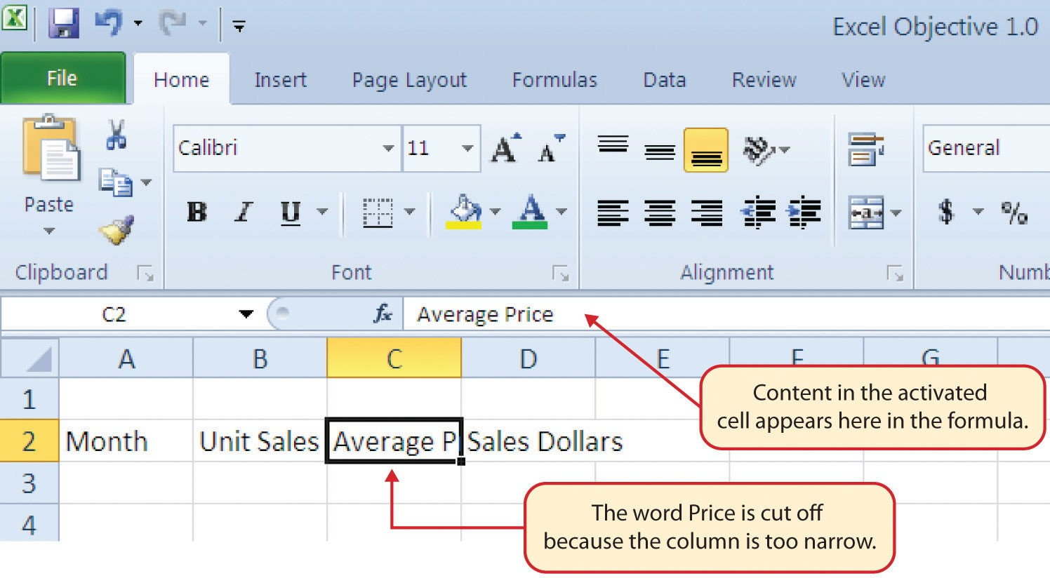
You will begin building the workbook shown in Figure 1.1 by manually entering data into the worksheet. The following steps explain how the column headings in Row 2 are typed into the worksheet:
- Click cell location A2 on the worksheet.
- Type the word Month.
- Press the RIGHT ARROW key. This will enter the word into cell A2 and activate the next cell to the right.
- Type Unit Sales and press the RIGHT ARROW key.
- Repeat step 4 for the words Average Price and then again for Sales Dollars.
Figure 1.15 shows how your worksheet should appear after you have typed the column headings into Row 2. Notice that the word Price in cell location C2 is not visible. This is because the column is too narrow to fit the entry you typed. We will examine formatting techniques to correct this problem in the next section.
Integrity Check
Column Headings
It is critical to include column headings that accurately describe the data in each column of a worksheet. In professional environments, you will likely be sharing Excel workbooks with coworkers. Good column headings reduce the chance of someone misinterpreting the data contained in a worksheet, which could lead to costly errors depending on your career.
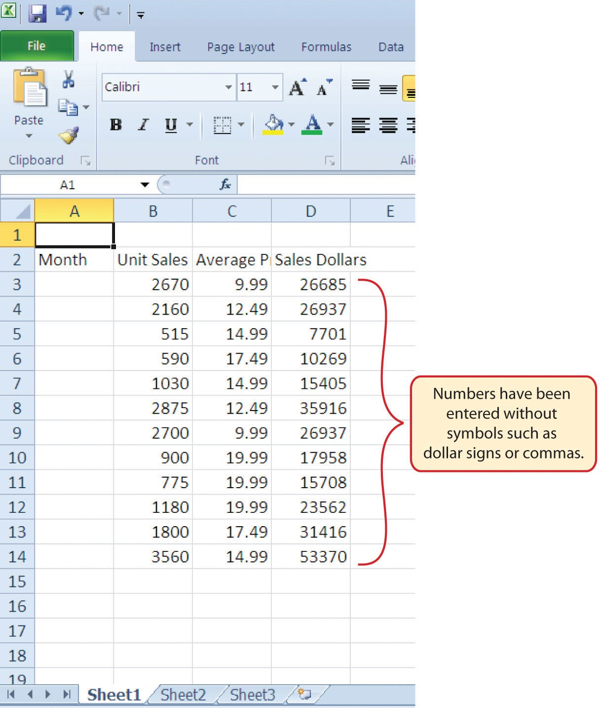
- Click cell location B3.
- Type the number 2670 and press the ENTER key. After you press the ENTER key, cell B4 will be activated. Using the ENTER key is an efficient way to enter data vertically down a column.
- Enter the following numbers in cells B4 through B14: 2160, 515, 590, 1030, 2875, 2700, 900, 775, 1180, 1800, and 3560.
- Click cell location C3.
- Type the number 9.99 and press the ENTER key.
- Enter the following numbers in cells C4 through C14: 12.49, 14.99, 17.49, 14.99, 12.49, 9.99, 19.99, 19.99, 19.99, 17.49, and 14.99.
- Activate cell location D3.
- Type the number 26685 and press the ENTER key.
- Enter the following numbers in cells D4 through D14: 26937, 7701, 10269, 15405, 35916, 26937, 17958, 15708, 23562, 31416, and 53370.
- When finished, check that the data you entered matches Figure 1.16.
Why?
Avoid Formatting Symbols When Entering Numbers
When typing numbers into an Excel worksheet, it is best to avoid adding any formatting symbols such as dollar signs and commas. Although Excel allows you to add these symbols while typing numbers, it slows down the process of entering data. It is more efficient to use Excel’s formatting features to add these symbols to numbers after you type them into a worksheet.
Integrity Check
Data Entry
It is very important to proofread your worksheet carefully, especially when you have entered numbers. Transposing numbers when entering data manually into a worksheet is a common error. For example, the number 563 could be transposed to 536. Such errors can seriously compromise the integrity of your workbook.
Integrity Check
Figure 1.16 shows how your worksheet should appear after entering the data. Check your numbers carefully to make sure they are accurately entered into the worksheet.
Editing Data
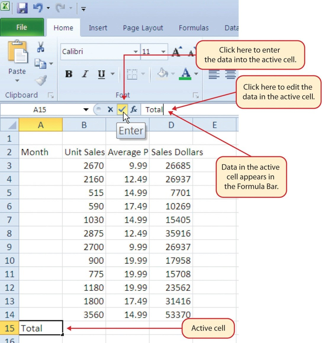
Data that has been entered in a cell can be changed by double clicking the cell location or using the Formula Bar. You may have noticed that as you were typing data into a cell location, the data you typed appeared in the Formula Bar. The Formula Bar can be used for entering data into cells as well as for editing data that already exists in a cell. The following steps provide an example of entering and then editing data that has been entered into a cell location:
- Click cell A15 in the Sheet1 worksheet.
- Type the abbreviation Tot and press the ENTER key.
- Click cell A15.
- Move the mouse pointer up to the Formula Bar. You will see the pointer turn into a cursor. Move the cursor to the end of the abbreviation Tot and left click.
- Type the letters al to complete the word Total.
- Click the checkmark to the left of the Formula Bar (see Figure 1.17). This will enter the change into the cell.

Figure 1.17 Using the Formula Bar to Edit and Enter Data - Double click cell A15.
- Add a space after the word Total and type the word Sales.
- Press the ENTER key.
Keyboard Shortcuts
Editing Data in a Cell
- Activate the cell that is to be edited and press the F2 key on your keyboard.
Auto Fill
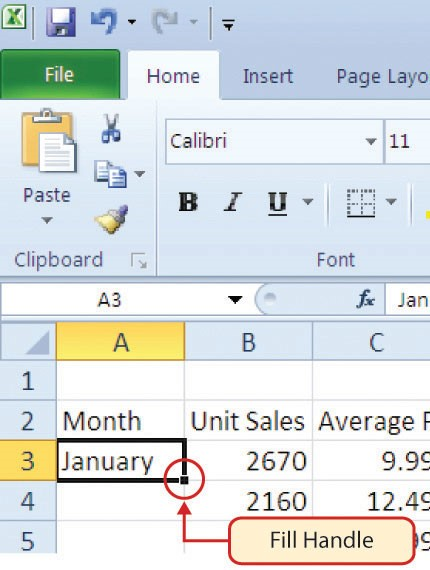
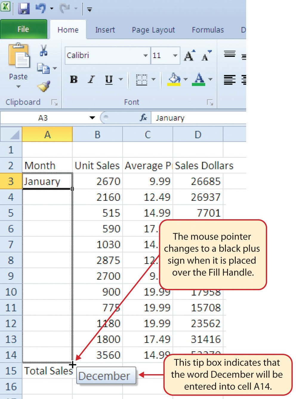
The Auto Fill feature is a valuable tool when manually entering data into a worksheet. This feature has many uses, but it is most beneficial when you are entering data in a defined sequence, such as the numbers 2, 4, 6, 8, and so on, or nonnumeric data such as the days of the week or months of the year. The following steps demonstrate how Auto Fill can be used to enter the months of the year in Column A:
- Click cell A3 in the Sheet1 worksheet.
- Type the word January and press the ENTER key.
- Activate cell A3 again.
- Move the mouse pointer to the lower right corner of cell A3. You will see a small square in this corner of the cell; this is called the Fill Handle (See Figure 1.18) When the mouse pointer gets close to the Fill Handle, the white block plus sign will turn into a black plus sign.
Left click and drag the Fill Handle to cell A14. Notice that the Auto Fill tip box indicates what month will be placed into each cell (see Figure 1.19). Release the left mouse button when the tip box reads “December.”
Once you release the left mouse button, all twelve months of the year should appear in the cell range A3:A14, as shown in Figure 1.20. You will also see the Auto Fill Options button. By clicking this button, you have several options for inserting data into a group of cells.
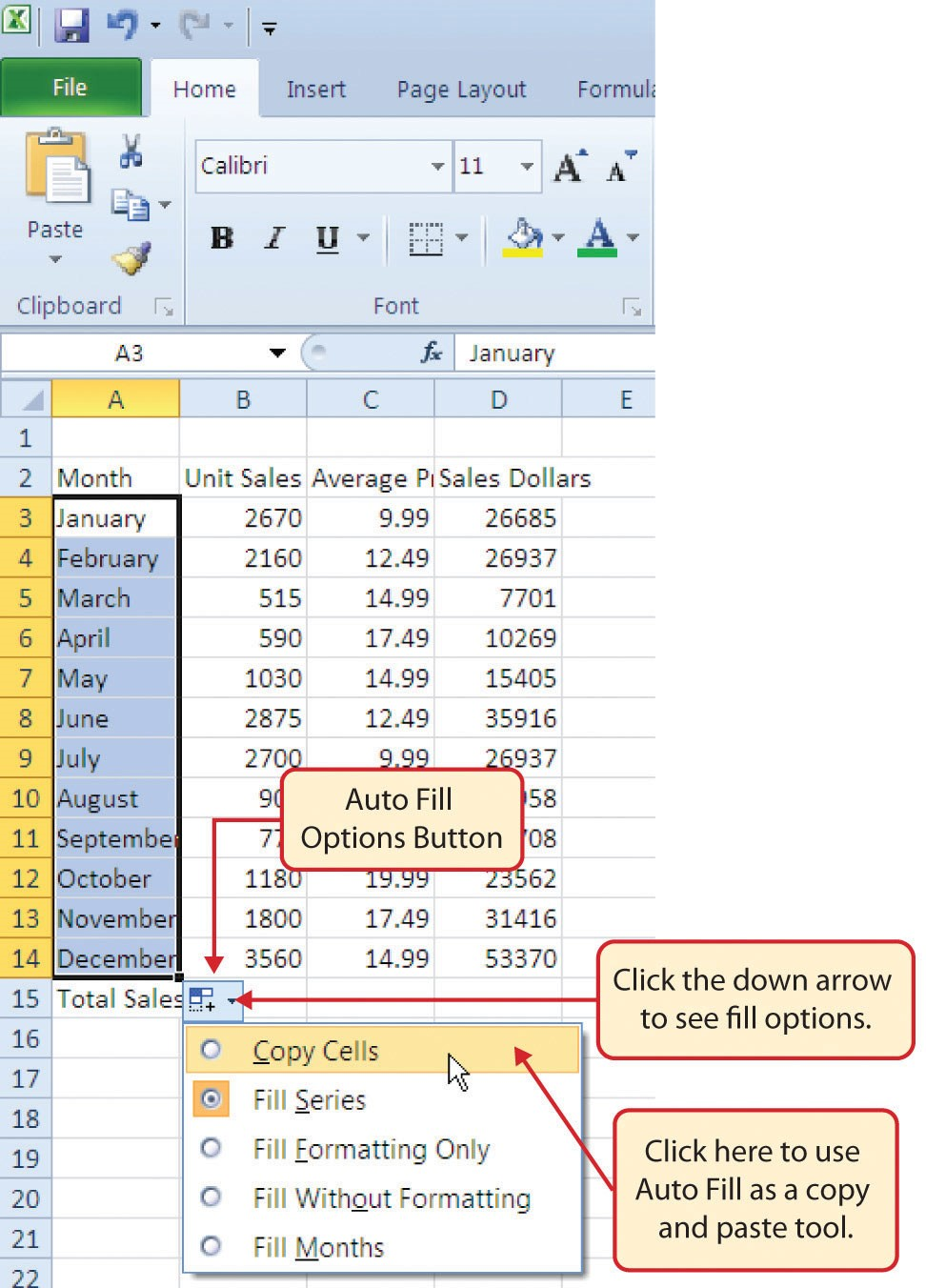
- Click the Auto Fill Options button.
- Click the Copy Cells option. This will change the months in the range A4:A14 to January.
- Click the Auto Fill Options button again.
- Click the Fill Months option to return the months of the year to the cell range A4:A14. The Fill Series option will provide the same result.
Deleting Data and the Undo Command
There are several methods for removing data from a worksheet, a few of which are demonstrated here. With each method, you use the Undo command. This is a helpful command in the event you mistakenly remove data from your worksheet. The following steps demonstrate how you can delete data from a cell or range of cells:
- Click cell C2 by placing the mouse pointer over the cell and clicking the left mouse button.
- Press the DELETE key on your keyboard. This removes the contents of the cell.
- Highlight the range C3:C14 by placing the mouse pointer over cell C3. Then left click and drag the mouse pointer down to cell C14.
- Place the mouse pointer over the Fill Handle. You will see the white block plus sign change to a black plus sign.
- Click and drag the mouse pointer up to cell C3 (see Figure 1.21). Release the mouse button. The contents in the range C3:C14 will be removed.
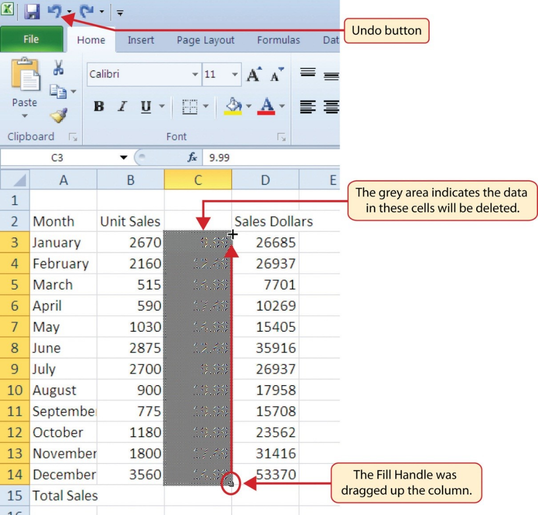
- Click the Undo button in the Quick Access Toolbar (see Figure 1.2). This should replace the data in the range C3:C14.
- Click the Undo button again. This should replace the data in cell C2.
Keyboard Shortcuts
Undo Command
- Hold down the CTRL key while pressing the letter Z on your keyboard.
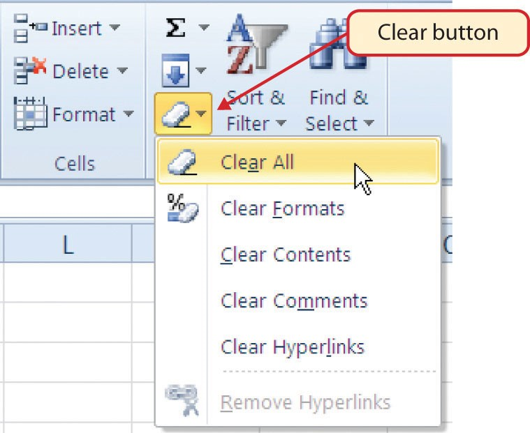
- Highlight the range C2:C14 by placing the mouse pointer over cell C2. Then left click and drag the mouse pointer down to cell C14.
- Click the Clear button in the Home tab of the Ribbon, which is next to the Cells group of commands (see Figure 1.22). This opens a drop-down menu that contains several options for removing or clearing data from a cell. Notice that you also have options for clearing just the formats in a cell or the hyperlinks in a cell.
- Click the Clear All option. This removes the data in the cell range.
- Click the Undo button. This replaces the data in the range C2:C14.
Adjusting Columns and Rows
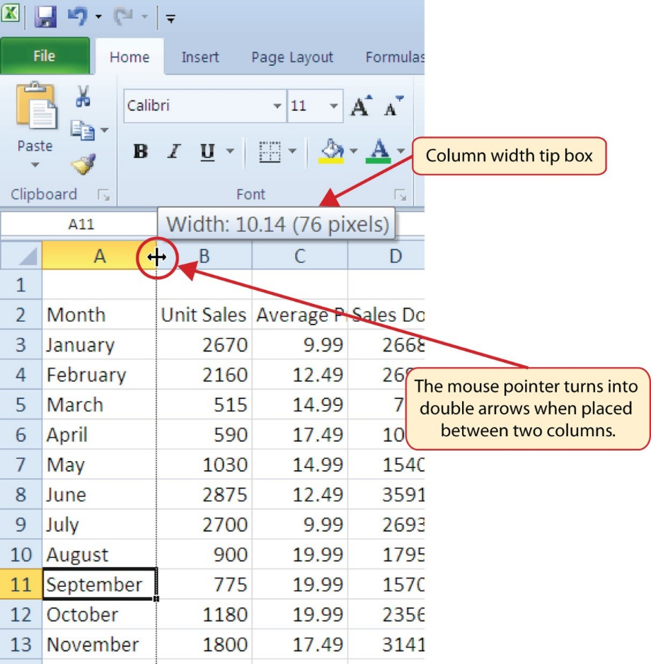
There are a few entries in the worksheet that appear cut off. For example, the last letter of the word September cannot be seen in cell A11. This is because the column is too narrow for this word. The columns and rows on an Excel worksheet can be adjusted to accommodate the data that is being entered into a cell. The following steps explain how to adjust the column widths and row heights in a worksheet:
- Bring the mouse pointer between Column A and Column B in the Sheet1 worksheet, as shown in Figure 1.23. You will see the white block plus sign turn into double arrows.
- Click and drag the column to the right so the entire word September in cell A11 can be seen. As you drag the column, you will see the column width tip box. This box displays the number of characters that will fit into the column using the Calibri 11-point font which is the default setting for font/size.
- Release the left mouse button.
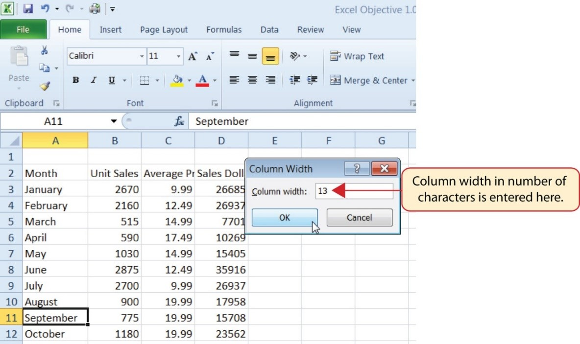
You may find that using the click-and-drag method is inefficient if you need to set a specific character width for one or more columns. Steps 1 through 6 illustrate a second method for adjusting column widths when using a specific number of characters:
- Click any cell location in Column A by moving the mouse pointer over a cell location and clicking the left mouse button. You can highlight cell locations in multiple columns if you are setting the same character width for more than one column.
- In the Home tab of the Ribbon, left click the Format button in the Cells group.
- Click the Column Width option from the drop-down menu. This will open the Column Width dialog box.
- Type the number 13 and click the OK button on the Column Width dialog box. This will set Column A to this character width (see Figure 1.24).
- Once again bring the mouse pointer between Column A and Column B so that the double arrow pointer displays and then double-click to activate AutoFit. This features adjusts the column width based on the longest entry in the column.
- Use the Column Width dialog box (step 6 above) to reset the width to 13.
Keyboard Shortcuts
Column Width
- Press the ALT key on your keyboard, then press the letters H, O, and W one at a time.
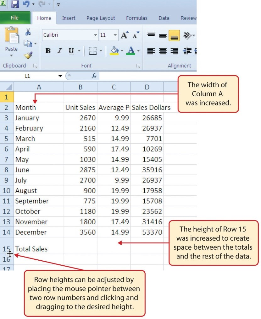
Steps 1 through 4 demonstrate how to adjust row height, which is similar to adjusting column width:
- Click cell A15 by placing the mouse pointer over the cell and clicking the left mouse button.
- In the Home tab of the Ribbon, left click the Format button in the Cells group.
- Click the Row Height option from the drop-down menu. This will open the Row Height dialog box.
- Type the number 24 and click the OK button on the Row Height dialog box. This will set Row 15 to a height of 24 points. A point is equivalent to approximately 1/72 of an inch. This adjustment in row height was made to create space between the totals for this worksheet and the rest of the data.
Keyboard Shortcuts
Row Height
- Press the ALT key on your keyboard, then press the letters H, O, and H one at a time.
Figure 1.25 shows the appearance of the worksheet after Column A and Row 15 are adjusted.
Skill Refresher
Adjusting Columns and Rows
- Activate at least one cell in the row or column you are adjusting.
- Click the Home tab of the Ribbon.
- Click the Format button in the Cells group.
- Click either Row Height or Column Width from the drop-down menu.
- Enter the Row Height in points or Column Width in characters in the dialog box.
- Click the OK button.
Hiding Columns and Rows
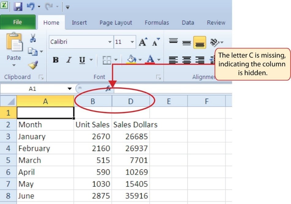
In addition to adjusting the columns and rows on a worksheet, you can also hide columns and rows. This is a useful technique for enhancing the visual appearance of a worksheet that contains data that is not necessary to display. These features will be demonstrated using the GMW Sales Data workbook. However, there is no need to have hidden columns or rows for this worksheet. The use of these skills here will be for demonstration purposes only.
- Click cell C1 in the Sheet1 worksheet by placing the mouse pointer over the cell location and clicking the left mouse button.
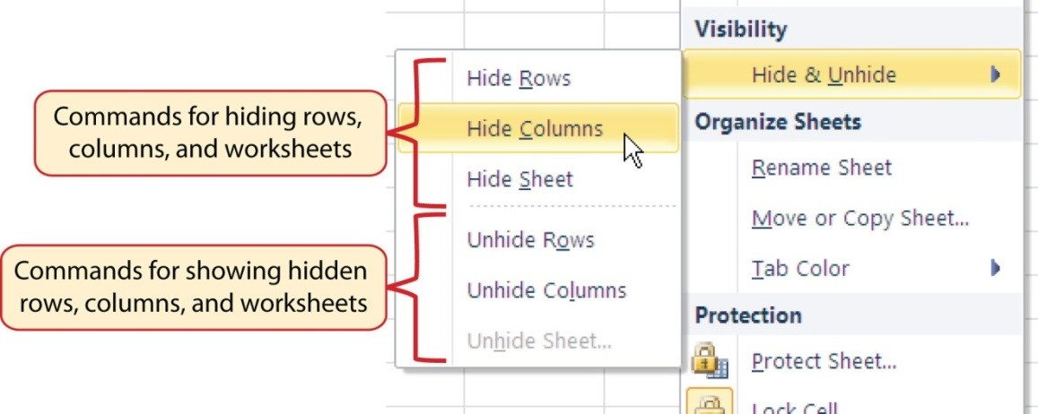
- Click the Format button in the Home tab of the Ribbon.
- Place the mouse pointer over the Hide & Unhide option in the drop-down menu. This will open a submenu of options.
- Click the Hide Columns option in the submenu of options (see Figure 1.26). This will hide Column C.
Keyboard Shortcuts
Hiding Columns
- Hold down the CTRL key while pressing the number 0 on your keyboard.
Figure 1.27 shows the workbook with Column C hidden in the Sheet1 worksheet. You can tell a column is hidden by the missing letter C.
To unhide a column, follow these steps:
- Highlight the range B1:D1 by activating cell B1 and clicking and dragging over to cell D1.
- Click the Format button in the Home tab of the Ribbon.
- Place the mouse pointer over the Hide & Unhide option in the drop-down menu.
- Click the Unhide Columns option in the submenu of options. Column C will now be visible on the worksheet.
Keyboard Shortcuts
Unhiding Columns
- Highlight cells on either side of the hidden column(s), then hold down the CTRL key and the SHIFT key while pressing the close parenthesis key ()) on your keyboard.
The following steps demonstrate how to hide rows, which is similar to hiding columns:
- Click cell A3 in the Sheet1 worksheet by placing the mouse pointer over the cell location and clicking the left mouse button.
- Click the Format button in the Home tab of the Ribbon.
- Place the mouse pointer over the Hide & Unhide option in the drop-down menu. This will open a submenu of options.
- Click the Hide Rows option in the submenu of options. This will hide Row 3.
Keyboard Shortcuts
Hiding Rows
- Hold down the CTRL key while pressing the number 9 key on your keyboard.
To unhide a row, follow these steps:
- Highlight the range A2:A4 by activating cell A2 and clicking and dragging over to cell A4.
- Click the Format button in the Home tab of the Ribbon.
- Place the mouse pointer over the Hide & Unhide option in the drop-down menu.
- Click the Unhide Rows option in the submenu of options. Row 3 will now be visible on the worksheet.
Keyboard Shortcuts
Unhiding Rows
- Highlight cells above and below the hidden row(s), then hold down the CTRL key and the SHIFT key while pressing the open parenthesis key (() on your keyboard.
Integrity Check
Hidden Rows and Columns
In most careers, it is common for professionals to use Excel workbooks that have been designed by a coworker. Before you use a workbook developed by someone else, always check for hidden rows and columns. You can quickly see whether a row or column is hidden if a row number or column letter is missing.
Skill Refresher
Hiding Columns and Rows
- Activate at least one cell in the row(s) or column(s) you are hiding.
- Click the Home tab of the Ribbon.
- Click the Format button in the Cells group.
- Place the mouse pointer over the Hide & Unhide option.
- Click either the Hide Rows or Hide Columns option.
Skill Refresher
Unhiding Columns and Rows
- Highlight the cells above and below the hidden row(s) or to the left and right of the hidden column(s).
- Click the Home tab of the Ribbon.
- Click the Format button in the Cells group.
- Place the mouse pointer over the Hide & Unhide option.
- Click either the Unhide Rows or Unhide Columns option.
Inserting Columns and Rows
Using Excel workbooks that have been created by others is a very efficient way to work because it eliminates the need to create data worksheets from scratch. However, you may find that to accomplish your goals, you need to add additional columns or rows of data. In this case, you can insert blank columns or rows into a worksheet. The following steps demonstrate how to do this:
- Click cell C1 in the Sheet1 worksheet by placing the mouse pointer over the cell location and clicking the left mouse button.
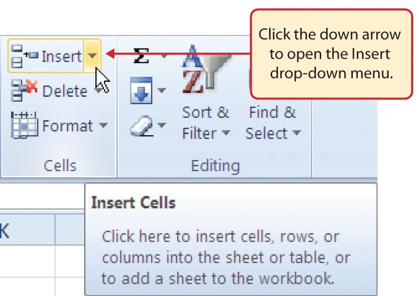
- Click the down arrow on the Insert button in the Home tab of the Ribbon (see Figure 1.28).

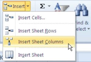
Figure 1.28 Insert Button (Down Arrow) - Click the Insert Sheet Columns option from the drop-down menu (see Figure 1.29). A blank column will be inserted to the left of Column C. The contents that were previously in Column C now appear in Column D. Note that columns are always inserted to the left of the activated cell.

Figure 1.29 Insert Drop-Down Menu Keyboard Shortcuts
Inserting Columns
- Press the ALT key and then the letters H, I, and C one at a time. A column will be inserted to the left of the activated cell.
- Click cell A3 in the Sheet1 worksheet by placing the mouse pointer over the cell location and clicking the left mouse button.
- Click the down arrow on the Insert button in the Home tab of the Ribbon (see Figure 1.28).
- Click the Insert Sheet Rows option from the drop-down menu (see Figure 1.29). A blank row will be inserted above Row 3. The contents that were previously in Row 3 now appear in Row 4. Note that rows are always inserted above the activated cell.
Keyboard Shortcuts
Inserting Rows
- Press the ALT key and then the letters H, I, and R one at a time. A row will be inserted above the activated cell.
Skill Refresher
Inserting Columns and Rows
- Activate the cell to the right of the desired blank column or below the desired blank row.
- Click the Home tab of the Ribbon.
- Click the down arrow on the Insert button in the Cells group.
- Click either the Insert Sheet Columns or Insert Sheet Rows option.
Moving Data
Once data are entered into a worksheet, you have the ability to move it to different locations. The following steps demonstrate how to move data to different locations on a worksheet:
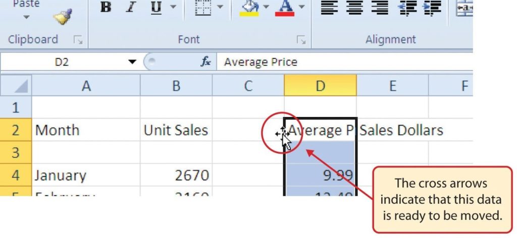
- Highlight the range D2:D15 by activating cell D2 and clicking and dragging down to cell D15.
- Bring the mouse pointer to the left edge of cell D2. You will see the white block plus sign change to cross arrows (see Figure 1.30). This indicates that you can left click and drag the data to a new location.

Figure 1.30 Moving Data - Left Click and drag the mouse pointer to cell C2.
- Release the left mouse button. The data now appears in Column C.
- Click the Undo button in the Quick Access Toolbar. This moves the data back to Column D.
Integrity Check
Moving Data
Before moving data on a worksheet, make sure you identify all the components that belong with the series you are moving. For example, if you are moving a column of data, make sure the column heading is included. Also, make sure all values are highlighted in the column before moving it.
Deleting Columns and Rows
You may need to delete entire columns or rows of data from a worksheet. This need may arise if you need to remove either blank columns or rows from a worksheet or columns and rows that contain data. The methods for removing cell contents were covered earlier and can be used to delete unwanted data. However, if you do not want a blank row or column in your workbook, you can delete it using the following steps:
- Click cell A3 by placing the mouse pointer over the cell location and clicking the left mouse button.
- Click the down arrow on the Delete button in the Cells group in the Home tab of the Ribbon.
- Click the Delete Sheet Rows option from the drop-down menu (see Figure 1.31). This removes Row 3 and shifts all the data (below Row 2) in the worksheet up one row.
Keyboard Shortcuts
Deleting Rows
- Press the ALT key and then the letters H, D, and R one at a time. The row with the activated cell will be deleted.

Figure 1.31 Delete Drop-Down Menu - Click cell C1 by placing the mouse pointer over the cell location and clicking the left mouse button.
- Click the down arrow on the Delete button in the Cells group in the Home tab of the Ribbon.
- Click the Delete Sheet Columns option from the drop-down menu (see Figure 1.31). This removes Column C and shifts all the data in the worksheet (to the right of Column B) over one column to the left.
- Save the changes to your workbook by clicking either the Save button on the Home ribbon; or by selecting the Save option from the File menu.

Keyboard Shortcuts
Deleting Columns
- Press the ALT key and then the letters H, D, and C one at a time. The column with the activated cell will be deleted.
Skill Refresher
Deleting Columns and Rows
- Activate any cell in the row or column that is to be deleted.
- Click the Home tab of the Ribbon.
- Click the down arrow on the Delete button in the Cells group.
- Click either the Delete Sheet Columns or the Delete Sheet Rows option.
Key Takeaways
- Column headings should be used in a worksheet and should accurately describe the data contained in each column.
- Using symbols such as dollar signs when entering numbers into a worksheet can slow down the data entry process.
- Worksheets must be carefully proofread when data has been manually entered.
- The Undo command is a valuable tool for recovering data that was deleted from a worksheet.
- When using a worksheet that was developed by someone else, look carefully for hidden columns or rows.
Attribution
Adapted by Barbara Lave from How to Use Microsoft Excel: The Careers in Practice Series, adapted by The Saylor Foundation without attribution as requested by the work’s original creator or licensee, and licensed under CC BY-NC-SA 3.0.