
Содержание
- Start a new line of text inside a cell in Excel
- Need more help?
- Insert or delete rows, and columns
- Insert or delete a column
- Insert or delete a row
- Formatting options
- Insert rows
- Insert columns
- Delete cells, rows, or columns
- Insert cells
- Need more help?
- 5 Keyboard Shortcuts for Rows and Columns in Excel
- #1 – Select Entire Row or Column
- #2 – Insert or Delete Rows or Columns
- #3 – AutoFit Column Width
- #3.5 – Manually Adjust Row or Column Width
- #4 – Hide or Unhide Rows or Columns
- #5 – Group or Ungroup Rows or Columns
- What Are Your Favorites?
Start a new line of text inside a cell in Excel
To start a new line of text or add spacing between lines or paragraphs of text in a worksheet cell, press Alt+Enter to insert a line break.
Double-click the cell in which you want to insert a line break.
Click the location inside the selected cell where you want to break the line.
Press Alt+Enter to insert the line break.
To start a new line of text or add spacing between lines or paragraphs of text in a worksheet cell, press CONTROL + OPTION + RETURN to insert a line break.
Double-click the cell in which you want to insert a line break.
Click the location inside the selected cell where you want to break the line.
Press CONTROL+OPTION+RETURN to insert the line break.
To start a new line of text or add spacing between lines or paragraphs of text in a worksheet cell, press Alt+Enter to insert a line break.
Double-click the cell in which you want to insert a line break (or select the cell and then press F2).
Click the location inside the selected cell where you want to break the line.
Press Alt+Enter to insert the line break.
Double-tap within the cell.
Tap the place where you want a line break, and then tap the blue cursor.

Tap New Line in the contextual menu.
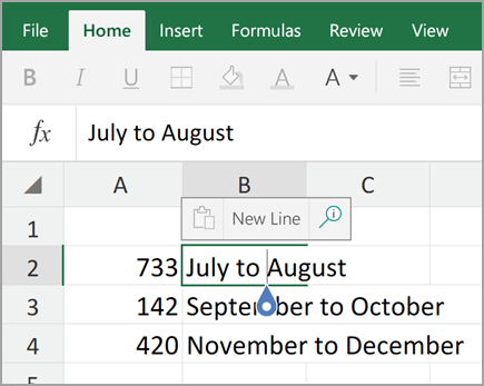
Note: You cannot start a new line of text in Excel for iPhone.
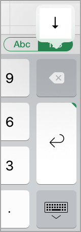
Tap the keyboard toggle button to open the numeric keyboard.

Press and hold the return key to view the line break key, and then drag your finger to that key.
Need more help?
You can always ask an expert in the Excel Tech Community or get support in the Answers community.
Источник
Insert or delete rows, and columns
Insert and delete rows and columns to organize your worksheet better.

Note: Microsoft Excel has the following column and row limits: 16,384 columns wide by 1,048,576 rows tall.
Insert or delete a column
Select any cell within the column, then go to Home > Insert > Insert Sheet Columns or Delete Sheet Columns.
Alternatively, right-click the top of the column, and then select Insert or Delete.
Insert or delete a row
Select any cell within the row, then go to Home > Insert > Insert Sheet Rows or Delete Sheet Rows.
Alternatively, right-click the row number, and then select Insert or Delete.
Formatting options
When you select a row or column that has formatting applied, that formatting will be transferred to a new row or column that you insert. If you don’t want the formatting to be applied, you can select the Insert Options button after you insert, and choose from one of the options as follows:
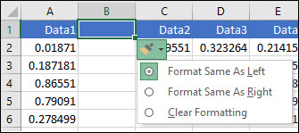
If the Insert Options button isn’t visible, then go to File > Options > Advanced > in the Cut, copy and paste group, check the Show Insert Options buttons option.
Insert rows
To insert a single row: Right-click the whole row above which you want to insert the new row, and then select Insert Rows.
To insert multiple rows: Select the same number of rows above which you want to add new ones. Right-click the selection, and then select Insert Rows.
Insert columns
To insert a single column: Right-click the whole column to the right of where you want to add the new column, and then select Insert Columns.
To insert multiple columns: Select the same number of columns to the right of where you want to add new ones. Right-click the selection, and then select Insert Columns.
Delete cells, rows, or columns
If you don’t need any of the existing cells, rows or columns, here’s how to delete them:
Select the cells, rows, or columns that you want to delete.
Right-click, and then select the appropriate delete option, for example, Delete Cells & Shift Up, Delete Cells & Shift Left, Delete Rows, or Delete Columns.
When you delete rows or columns, other rows or columns automatically shift up or to the left.
Tip: If you change your mind right after you deleted a cell, row, or column, just press Ctrl+ Z to restore it.
Insert cells
To insert a single cell:
Right-click the cell above which you want to insert a new cell.
Select Insert, and then select Cells & Shift Down.
To insert multiple cells:
Select the same number of cells above which you want to add the new ones.
Right-click the selection, and then select Insert > Cells & Shift Down.
Need more help?
You can always ask an expert in the Excel Tech Community or get support in the Answers community.
Источник
5 Keyboard Shortcuts for Rows and Columns in Excel
Bottom line: Learn some of my favorite keyboard shortcuts when working with rows and columns in Excel.
Skill level: Easy
Whether you are creating a simple list of names or building a complex financial model, you probably make a lot of changes to the rows and columns in the spreadsheet. Tasks like adding/deleting rows, adjusting column widths, and creating outline groups are very common when working with the grid.
This post contains some of my favorite shortcuts that will save you time every day.
I’ve also listed the equivalent shortcuts for the Mac version of Excel where available.
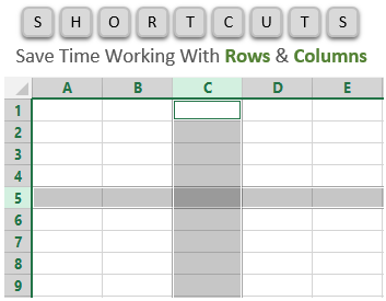
#1 – Select Entire Row or Column
Shift+Space is the keyboard shortcut to select an entire row.
Ctrl+Space is the keyboard shortcut to select an entire column.
Mac Shortcuts: Same as above
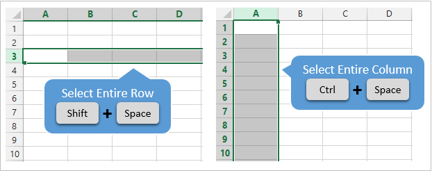
The keyboard shortcuts by themselves don’t do much. However, they are the starting point for performing a lot of other actions where you first need to select the entire row or column. This includes tasks like deleting rows, grouping columns, etc.
These shortcuts also work for selecting the entire row or column inside an Excel Table.
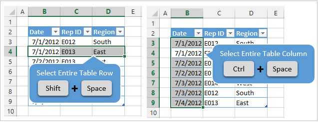
When you press the Shift+Space shortcut the first time it will select the entire row within the Table. Press Shift+Space a second time and it will select the entire row in the worksheet.
The same works for columns. Ctrl+Space will select the column of data in the Table. Pressing the keyboard shortcut a second time will include the column header of the Table in the selection. Pressing Ctrl+Space a third time will select the entire column in the worksheet.
You can select multiple rows or columns by holding Shift and pressing the Arrow Keys multiple times.
![]()
#2 – Insert or Delete Rows or Columns
There are a few ways to quickly delete rows and columns in Excel.
If you have the rows or columns selected, then the following keyboard shortcuts will quickly add or delete all selected rows or columns.
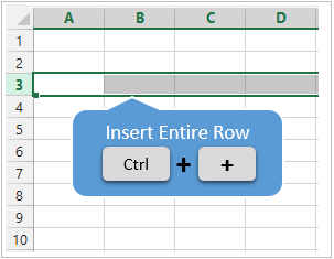
Ctrl++ (plus character) is the keyboard shortcut to insert rows or columns. If you are using a laptop keyboard you can press Ctrl+Shift+= (equal sign).
Mac Shortcut: Cmd++ or Cmd+Shift+
Ctrl+- (minus character) is the keyboard shortcut to delete rows or columns.
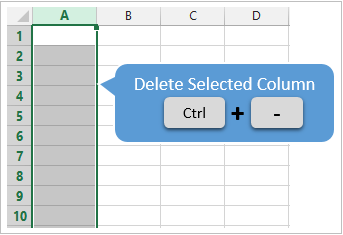
So for the above shortcuts to work you will first need to select the entire row or column, which can be done with the Shift+Space or Ctrl+Space shortcuts explained in #1.
If you do not have the entire row or column selected then you will be presented with the Insert or Delete Menus after pressing Ctrl++ or Ctrl+-.
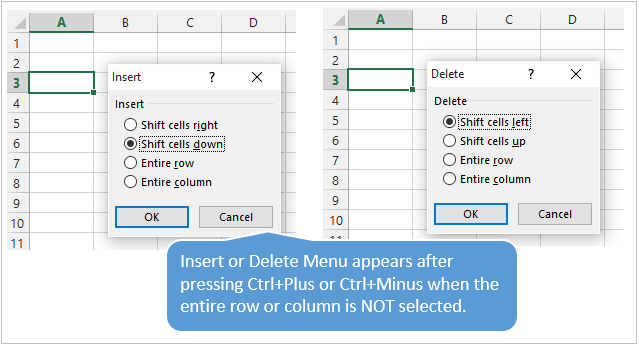
You can then press the up or down arrow keys to make your selection from the menu and hit Enter. For me it is easier to first select the entire row or column, then press Ctrl++ or Ctrl+-.
So, the entire keyboard shortcut to delete a column would be Ctrl+Space, Ctrl+-. You could also use the keyboard shortcut Alt+H+D+C to delete columns and Alt+H+D+R to delete rows. There are lots of ways to do a simple task… 🙂
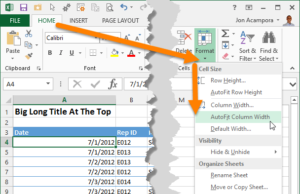
#3 – AutoFit Column Width
There are also a lot of different ways to AutoFit column widths. AutoFit means that the width of the column will be adjusted to fit the contents of the cell.
You can use the mouse and double-click when you hover the cursor between columns when you see the resize column cursor.
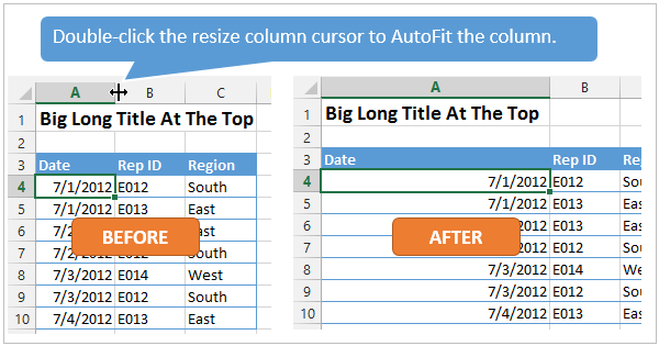
The problem with this is that you might just want to resize the column for the date in cell A4, instead of the big long title in cell A1. To accomplish this you can use the AutoFit Column Width button. It is located on the Home tab of the Ribbon in the Format menu.
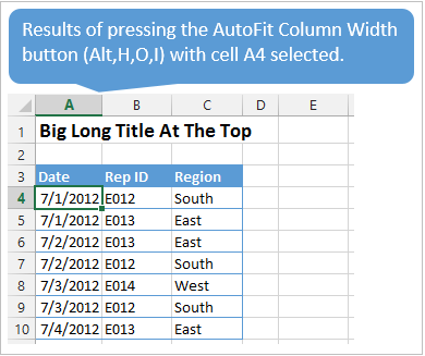
The AutoFit Column Width button bases the width of the column on the cells you have selected. In the image above I have cell A4 selected. So the column width will be adjusted to fit the contents of A4, as shown in the results below.
Alt,H,O,I is the keyboard shortcut for the AutoFit Column Width button. This is one I use a lot to get my reports looking shiny. 🙂
Alt,H,O,A is the keyboard shortcut to AutoFit Row Height. It doesn’t work exactly the same as column width, and will only adjust the row height to the tallest cell in the entire row.
Mac Shortcuts: None that I know of. The Mac version does not use the Alt key sequence which I believe is a limitation of the Mac OS.
#3.5 – Manually Adjust Row or Column Width
The column width or row height windows can be opened with keyboard shortcuts as well.
Alt,O,R,E is the keyboard shortcut to open the Row Height window.
Alt,O,C,W is the keyboard shortcut to open the Column Width window.
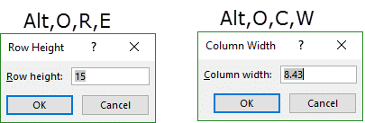
The row height or column width will be applied to the rows or columns of all the cells that are currently selected.
These are old shortcuts from Excel 2003, but they still work in the modern versions of Excel.
Mac Shortcuts: None that I know of. The Mac version does not use the Alt key sequence which I believe is a limitation of the Mac OS.
#4 – Hide or Unhide Rows or Columns
There are several dedicated keyboard shortcuts to hide and unhide rows and columns.
- Ctrl+9 to Hide Rows
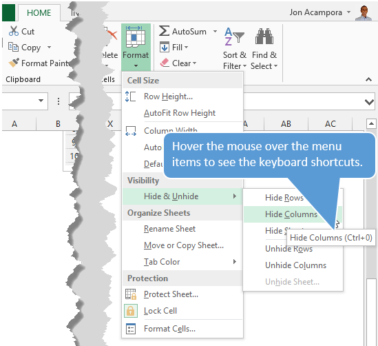
- Ctrl+0 (zero) to Hide Columns
- Ctrl+Shift+( to Unhide Rows
- Ctrl+Shift+) to Unhide Columns – If this doesn’t work for you try Alt,O,C,U (old Excel 2003 shortcut that still works). You can also modify a Windows setting to prevent the conflict with this shortcut. See the comment from Pablo Baez on Oct 5, 2015 below for further instructions. Thanks Pablo! 🙂
Mac Shortcuts: Same as above
The buttons are also located on the Format menu on the Home tab of the Ribbon. You can hover over any of the items in the menu and the keyboard shortcut will display in the screentip (see screenshot below).
The trick with getting these shortcuts to work is to have the proper cells selected first.
To hide rows or columns you just need to select cells in the rows or columns you want to hide, then press the Ctrl+9 or Ctrl+Shift+( shortcut.
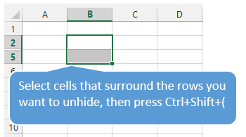
To unhide rows or columns you first need to select the cells that surround the rows or columns you want to unhide. In the screenshot below I want to unhide rows 3 & 4. I first select cell B2:B5, cells that surround or cover the hidden rows, then press Ctrl+Shift+( to unhide the rows.
The same technique works to unhide columns.
#5 – Group or Ungroup Rows or Columns
Row and Column groupings are a great way to quickly hide and unhide columns and rows.
Shift+Alt+Right Arrow is the shortcut to group rows or columns.
Mac Shortcut: Cmd+Shift+K
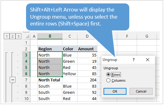
Shift+Alt+Left Arrow is the shortcut to ungroup.
Mac Shortcut: Cmd+Shift+J
Again, the trick here is to select the entire rows or columns you want to group/ungroup first. Otherwise you will be presented with the Group or Ungroup menu.
Alt,A,U,C is the keyboard shortcut to remove all the row and columns groups on the sheet. This is the same as pressing the Clear Outline button on the Ungroup menu of the Data tab on the Ribbon.
*Bonus funny: At some point when using the group/ungroup shortcuts, you will accidentally press Ctrl+Alt+Right Arrow. This is a Windows shortcut that orientates the entire screen to the right. I call it “neck ache view”. To get it back to normal press Ctrl+Alt+Up Arrow.
If your co-worker or boss accidentally leaves their computer unlocked and you want to play a joke on them, press Ctrl+Alt+Down Arrow. This will turn their screen upside down. Don’t forget to record a video of their WTF reaction… 🙂
What Are Your Favorites?
There are a ton of keyboard shortcuts for working with rows and columns. The above are some of my favorites that I use everyday. What are some of your favorites? Please leave a comment below. Thanks! 🙂
Источник
Insert or delete rows and columns
Insert and delete rows and columns to organize your worksheet better.
Note: Microsoft Excel has the following column and row limits: 16,384 columns wide by 1,048,576 rows tall.
Insert or delete a column
-
Select any cell within the column, then go to Home > Insert > Insert Sheet Columns or Delete Sheet Columns.
-
Alternatively, right-click the top of the column, and then select Insert or Delete.
Insert or delete a row
-
Select any cell within the row, then go to Home > Insert > Insert Sheet Rows or Delete Sheet Rows.
-
Alternatively, right-click the row number, and then select Insert or Delete.
Formatting options
When you select a row or column that has formatting applied, that formatting will be transferred to a new row or column that you insert. If you don’t want the formatting to be applied, you can select the Insert Options button after you insert, and choose from one of the options as follows:
If the Insert Options button isn’t visible, then go to File > Options > Advanced > in the Cut, copy and paste group, check the Show Insert Options buttons option.
Insert rows
To insert a single row: Right-click the whole row above which you want to insert the new row, and then select Insert Rows.
To insert multiple rows: Select the same number of rows above which you want to add new ones. Right-click the selection, and then select Insert Rows.
Insert columns
To insert a single column: Right-click the whole column to the right of where you want to add the new column, and then select Insert Columns.
To insert multiple columns: Select the same number of columns to the right of where you want to add new ones. Right-click the selection, and then select Insert Columns.
Delete cells, rows, or columns
If you don’t need any of the existing cells, rows or columns, here’s how to delete them:
-
Select the cells, rows, or columns that you want to delete.
-
Right-click, and then select the appropriate delete option, for example, Delete Cells & Shift Up, Delete Cells & Shift Left, Delete Rows, or Delete Columns.
When you delete rows or columns, other rows or columns automatically shift up or to the left.
Tip: If you change your mind right after you deleted a cell, row, or column, just press Ctrl+Z to restore it.
Insert cells
To insert a single cell:
-
Right-click the cell above which you want to insert a new cell.
-
Select Insert, and then select Cells & Shift Down.
To insert multiple cells:
-
Select the same number of cells above which you want to add the new ones.
-
Right-click the selection, and then select Insert > Cells & Shift Down.
Need more help?
You can always ask an expert in the Excel Tech Community or get support in the Answers community.
See Also
Basic tasks in Excel
Overview of formulas in Excel
Need more help?
Want more options?
Explore subscription benefits, browse training courses, learn how to secure your device, and more.
Communities help you ask and answer questions, give feedback, and hear from experts with rich knowledge.

Как известно, по умолчанию в одной ячейке листа Excel располагается одна строка с числами, текстом или другими данными. Но, что делать, если нужно перенести текст в пределах одной ячейки на другую строку? Данную задачу можно выполнить, воспользовавшись некоторыми возможностями программы. Давайте разберемся, как сделать перевод строки в ячейке в Excel.
Способы переноса текста
Некоторые пользователи пытаются перенести текст внутри ячейки нажатием на клавиатуре кнопки Enter. Но этим они добиваются только того, что курсор перемещается на следующую строку листа. Мы же рассмотрим варианты переноса именно внутри ячейки, как очень простые, так и более сложные.
Способ 1: использование клавиатуры
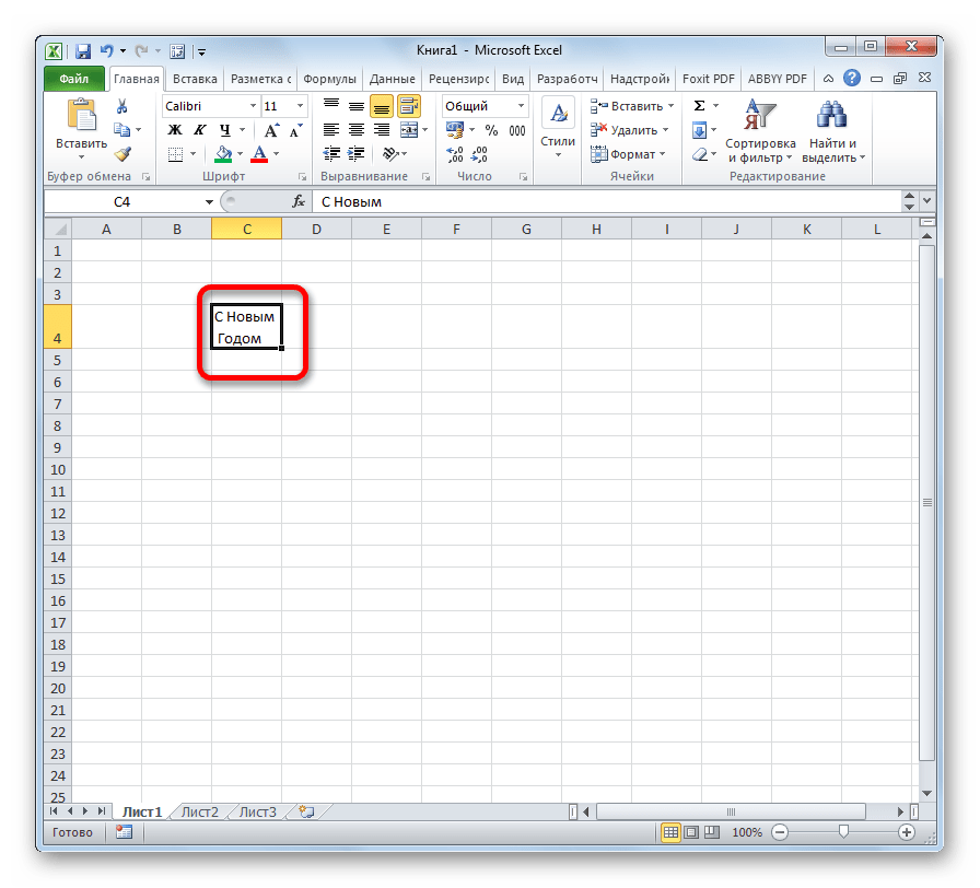
Самый простой вариант переноса на другую строку, это установить курсор перед тем отрезком, который нужно перенести, а затем набрать на клавиатуре сочетание клавиш Alt+Enter.
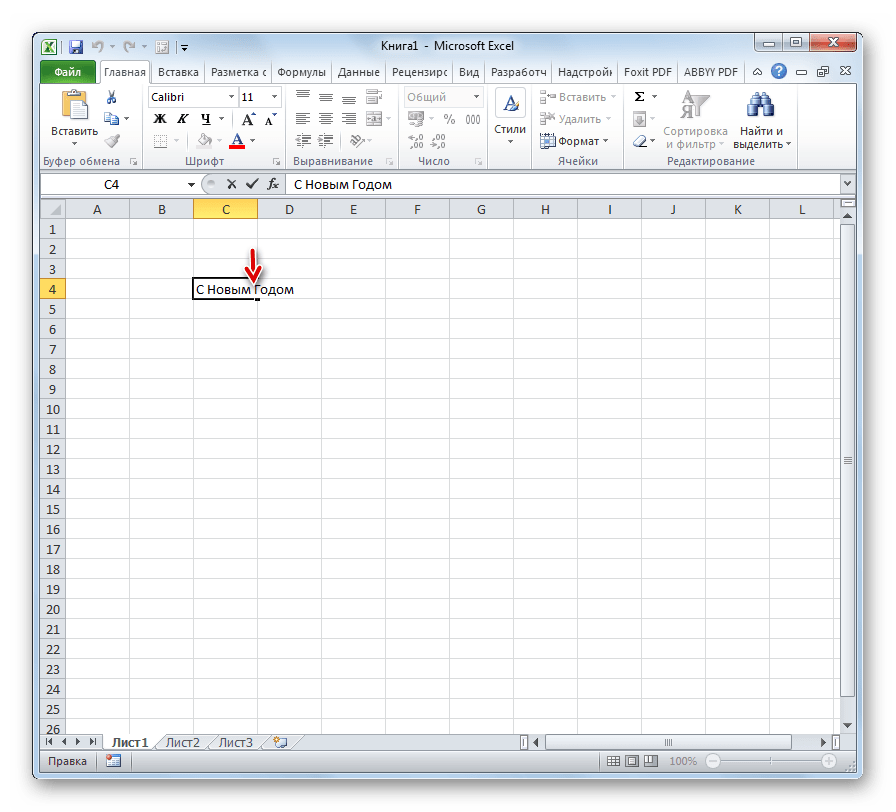
В отличие от использования только одной кнопки Enter, с помощью этого способа будет достигнут именно такой результат, который ставится.
Способ 2: форматирование
Если перед пользователем не ставится задачи перенести на новую строку строго определенные слова, а нужно только уместить их в пределах одной ячейки, не выходя за её границы, то можно воспользоваться инструментом форматирования.
-
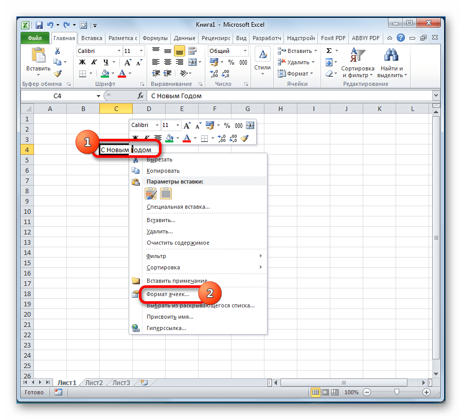
Выделяем ячейку, в которой текст выходит за пределы границ. Кликаем по ней правой кнопкой мыши. В открывшемся списке выбираем пункт «Формат ячеек…».
После этого, если данные будут выступать за границы ячейки, то она автоматически расширится в высоту, а слова станут переноситься. Иногда приходится расширять границы вручную.
Чтобы подобным образом не форматировать каждый отдельный элемент, можно сразу выделить целую область. Недостаток данного варианта заключается в том, что перенос выполняется только в том случае, если слова не будут вмещаться в границы, к тому же разбитие осуществляется автоматически без учета желания пользователя.
Способ 3: использование формулы
Также можно осуществить перенос внутри ячейки при помощи формул. Этот вариант особенно актуален в том случае, если содержимое выводится с помощью функций, но его можно применять и в обычных случаях.
- Отформатируйте ячейку, как указано в предыдущем варианте.
- Выделите ячейку и введите в неё или в строку формул следующее выражение:
Вместо элементов «ТЕКСТ1» и «ТЕКСТ2» нужно подставить слова или наборы слов, которые хотите перенести. Остальные символы формулы изменять не нужно.
Главным недостатком данного способа является тот факт, что он сложнее в выполнении, чем предыдущие варианты.
В целом пользователь должен сам решить, каким из предложенных способов оптимальнее воспользоваться в конкретном случае. Если вы хотите только, чтобы все символы вмещались в границы ячейки, то просто отформатируйте её нужным образом, а лучше всего отформатировать весь диапазон. Если вы хотите устроить перенос конкретных слов, то наберите соответствующее сочетание клавиш, как рассказано в описании первого способа. Третий вариант рекомендуется использовать только тогда, когда данные подтягиваются из других диапазонов с помощью формулы. В остальных случаях использование данного способа является нерациональным, так как имеются гораздо более простые варианты решения поставленной задачи.
Отблагодарите автора, поделитесь статьей в социальных сетях.

Довольно часто возникает вопрос, как сделать перенос на другую строку внутри ячейки в Экселе? Этот вопрос возникает когда текст в ячейке слишком длинный, либо перенос необходим для структуризации данных. В таком случае бывает не удобно работать с таблицами. Обычно перенос текста осуществляется с помощью клавиши Enter. Например, в программе Microsoft Office Word. Но в Microsoft Office Excel при нажатии на Enter мы попадаем на соседнюю нижнюю ячейку.
Итак нам требуется осуществить перенос текста на другую строку. Для переноса нужно нажать сочетание клавиш Alt+Enter. После чего слово, находящееся с правой стороны от курсора перенесется на следующую строку.

Автоматический перенос текста в Excel
В Экселе на вкладке Главная в группе Выравнивание есть кнопка «Перенос текста». Если выделить ячейку и нажать эту кнопку, то текст в ячейке будет переноситься на новую строку автоматически в зависимости от ширины ячейки. Для автоматического переноса требуется выполнить простое нажатие кнопки.

Убрать перенос с помощью функции и символа переноса
Для того, что бы убрать перенос мы можем использовать функцию ПОДСТАВИТЬ.
Функция заменяет один текст на другой в указанной ячейке. В нашем случае мы будем заменять символ пробел на символ переноса.
=ПОДСТАВИТЬ (текст;стар_текст;нов_текст;[номер вхождения])
Итоговый вид формулы:
- А1 – ячейка содержащая текст с переносами,
- СИМВОЛ(10) – символ переноса строки,
- » » – пробел.

Если же нам наоборот требуется вставить символ переноса на другую строку, вместо пробела проделаем данную операцию наоборот.
Что бы функция работало корректно во вкладке Выравнивание (Формат ячеек) должен быть установлен флажок «Переносить по словам».
Перенос с использование формулы СЦЕПИТЬ
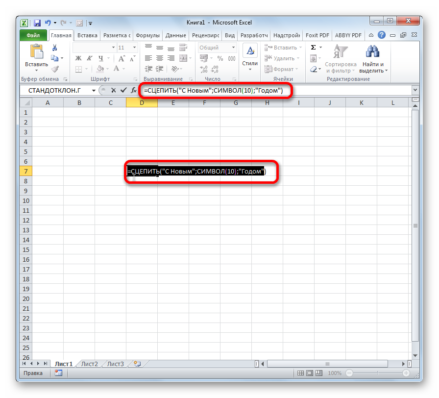
Для решения нашей проблемы можно использовать формулу СЦЕПИТЬ.
У нас имеется текст в ячейках A1 и B1. Введем в B3 следующую формулу:

Как в примере, который я приводил выше, для корректной работы функции в свойствах требуется установить флажок «переносить по словам».
Часто требуется внутри одной ячейки Excel сделать перенос текста на новую строку. То есть переместить текст по строкам внутри одной ячейки как указано на картинке. Если после ввода первой части текста просто нажать на клавишу ENTER, то курсор будет перенесен на следующую строку, но другую ячейку, а нам требуется перенос в этой же ячейке.

Это очень частая задача и решается она очень просто — для переноса текста на новую строку внутри одной ячейки Excel необходимо нажать ALT+ENTER (зажимаете клавишу ALT, затем не отпуская ее, нажимаете клавишу ENTER)
Как перенести текст на новую строку в Excel с помощью формулы
Иногда требуется сделать перенос строки не разово, а с помощью функций в Excel. Вот как в этом примере на рисунке. Мы вводим имя, фамилию и отчество и оно автоматически собирается в ячейке A6

Для начала нам необходимо сцепить текст в ячейках A1 и B1 ( A1&B1 ), A2 и B2 ( A2&B2 ), A3 и B3 ( A3&B3 )
После этого объединим все эти пары, но так же нам необходимо между этими парами поставить символ (код) переноса строки. Есть специальная таблица знаков (таблица есть в конце данной статьи), которые можно вывести в Excel с помощью специальной функции СИМВОЛ(число), где число это число от 1 до 255, определяющее определенный знак.
Например, если прописать =СИМВОЛ(169), то мы получим знак копирайта ©
Нам же требуется знак переноса строки, он соответствует порядковому номеру 10 — это надо запомнить.
Код (символ) переноса строки — 10
Следовательно перенос строки в Excel в виде функции будет выглядеть вот так СИМВОЛ(10)
Примечание: В VBA Excel перенос строки вводится с помощью функции Chr и выглядит как Chr (10)
Итак, в ячейке A6 пропишем формулу
= A1&B1 &СИМВОЛ(10)& A2&B2 &СИМВОЛ(10)& A3&B3
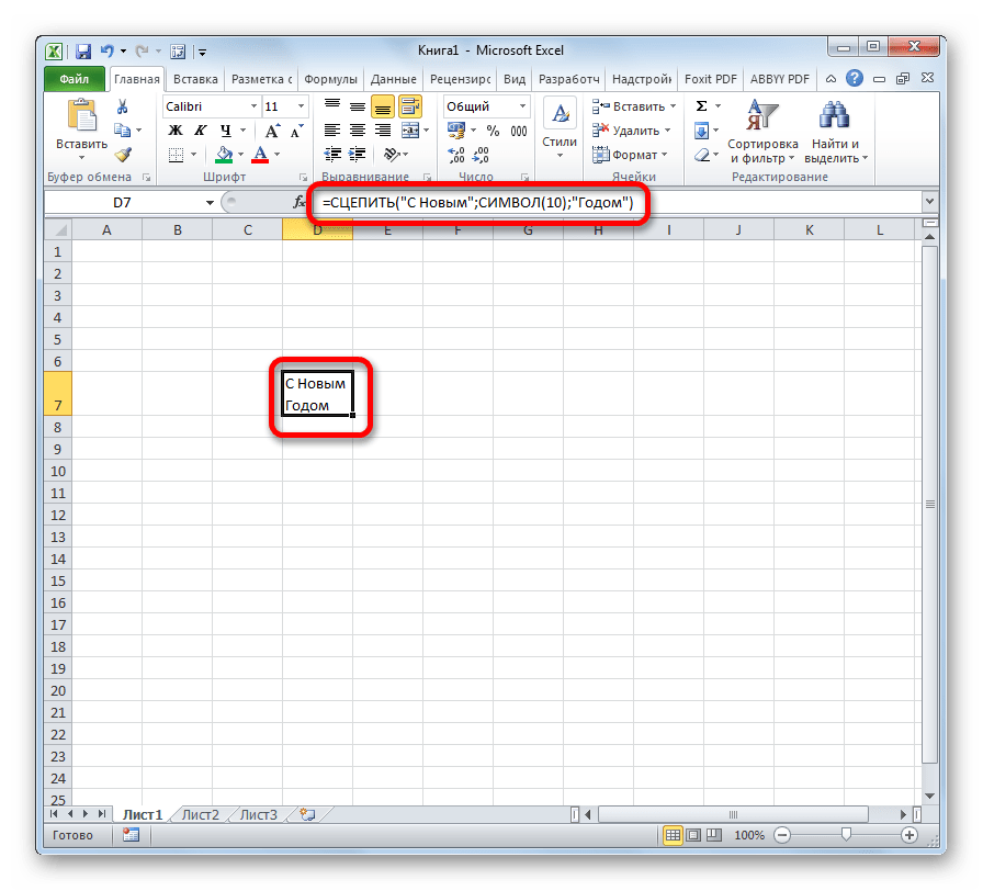
В итоге мы должны получить нужный нам результат.
Обратите внимание! Чтобы перенос строки корректно отображался необходимо включить «перенос по строкам» в свойствах ячейки.
Для этого выделите нужную нам ячейку (ячейки), нажмите на правую кнопку мыши и выберите «Формат ячеек. » 
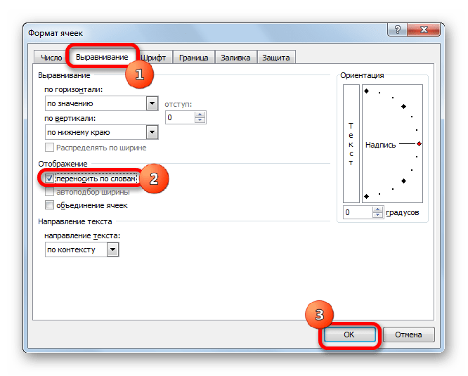
В открывшемся окне во вкладке «Выравнивание» необходимо поставить галочку напротив «Переносить по словам» как указано на картинке, иначе перенос строк в Excel не будет корректно отображаться с помощью формул.

Как в Excel заменить знак переноса на другой символ и обратно с помощью формулы
Можно поменять символ перенос на любой другой знак, например на пробел, с помощью текстовой функции ПОДСТАВИТЬ в Excel

Рассмотрим на примере, что на картинке выше. Итак, в ячейке B1 прописываем функцию ПОДСТАВИТЬ:
A1 — это наш текст с переносом строки;
СИМВОЛ(10) — это перенос строки (мы рассматривали это чуть выше в данной статье);
» » — это пробел, так как мы меняем перенос строки на пробел
Если нужно проделать обратную операцию — поменять пробел на знак (символ) переноса, то функция будет выглядеть соответственно:
Напоминаю, чтобы перенос строк правильно отражался, необходимо в свойствах ячеек, в разделе «Выравнивание» указать «Переносить по строкам».
Как поменять знак переноса на пробел и обратно в Excel с помощью ПОИСК — ЗАМЕНА
Бывают случаи, когда формулы использовать неудобно и требуется сделать замену быстро. Для этого воспользуемся Поиском и Заменой. Выделяем наш текст и нажимаем CTRL+H, появится следующее окно.

Если нам необходимо поменять перенос строки на пробел, то в строке «Найти» необходимо ввести перенос строки, для этого встаньте в поле «Найти», затем нажмите на клавишу ALT , не отпуская ее наберите на клавиатуре 010 — это код переноса строки, он не будет виден в данном поле.
После этого в поле «Заменить на» введите пробел или любой другой символ на который вам необходимо поменять и нажмите «Заменить» или «Заменить все».
Кстати, в Word это реализовано более наглядно.
Если вам необходимо поменять символ переноса строки на пробел, то в поле «Найти» вам необходимо указать специальный код «Разрыва строки», который обозначается как ^l
В поле «Заменить на: » необходимо сделать просто пробел и нажать на «Заменить» или «Заменить все».

Вы можете менять не только перенос строки, но и другие специальные символы, чтобы получить их соответствующий код, необходимо нажать на кнопку «Больше >> «, «Специальные» и выбрать необходимый вам код. Напоминаю, что данная функция есть только в Word, в Excel эти символы не будут работать.

Как поменять перенос строки на пробел или наоборот в Excel с помощью VBA
Рассмотрим пример для выделенных ячеек. То есть мы выделяем требуемые ячейки и запускаем макрос
1. Меняем пробелы на переносы в выделенных ячейках с помощью VBA
Sub ПробелыНаПереносы()
For Each cell In Selection
cell.Value = Replace (cell.Value, Chr (32) , Chr (10) )
Next
End Sub
2. Меняем переносы на пробелы в выделенных ячейках с помощью VBA
Sub ПереносыНаПробелы()
For Each cell In Selection
cell.Value = Replace (cell.Value, Chr (10) , Chr (32) )
Next
End Sub
Код очень простой Chr (10) — это перенос строки, Chr (32) — это пробел. Если требуется поменять на любой другой символ, то заменяете просто номер кода, соответствующий требуемому символу.
Коды символов для Excel
Ниже на картинке обозначены различные символы и соответствующие им коды, несколько столбцов — это различный шрифт. Для увеличения изображения, кликните по картинке.
-
#2
I tried Alt J… in the «other» box
Try Ctrl+J
-
#3
Thanks but that does not work.
-
#4
Hi
Should work if you composed the text in excel with the alt-enter.
Did you import the data?
For ex.: sometimes, if you import data, in some text sources the delimiter for the line is carriage return-linefeed and not just linefeed like in the excel cell.
Please check.
-
#5
Hi
Should work if you composed the text in excel with the alt-enter.
Did you import the data?
For ex.: sometimes, if you import data, in some text sources the delimiter for the line is carriage return-linefeed and not just linefeed like in the excel cell.
Please check.
I had a software pull this data from a website. I’m not sure about «linefeed».
-
#6
I’m thinking about another way around it. If I use the function =left(text,number) the first two are blank and the text starts at number 3. Any ideas to delete the first two?

Joe4
MrExcel MVP, Junior Admin
-
#7
I think the best way is to determine exactly what it is you are dealing with. So, we can get the ASCII number code for the character, and then use an ASCII table to see what we are working with.
Here is how you can do that. First, determine exactly where this «character» exists in your string. So, if it is in the 8th place of the entry in cell A1, use this formula to get the ASCII code:
=MID(A1,8,1)
Once we know the code, we can look up to see what it is: (Ascii Table — ASCII character codes and html, octal, hex and decimal chart conversion)
Once we know what it is, we can address it.
-
#8
I’m thinking about another way around it. If I use the function =left(text,number) the first two are blank and the text starts at number 3. Any ideas to delete the first two?
Hi
Use Find/Replace. Replace ?? with nothing.
-
#9
Hi
Use Find/Replace. Replace ?? with nothing.
Pedro, won’t that replace every pair of characters, not only the first 2 characters?
.. the first two are blank and the text starts at number 3
If that is consistent, then Text to Columns (Fixed width) should suffice.
If doing it manually, do Text to Columns -> Fixed width -> Click the ruler at position 2 -> Double click any other dividers that Excel may ave automatically inserted to remove them -> Next -> The 1st column of 2 characters should be highlighted so click ‘Do not import column’ -> Finish
If you want a macro to do that for you, try
Code:
Sub FixEm()
  Columns("A").TextToColumns DataType:=xlFixedWidth, FieldInfo:=Array(Array(0, 9), Array(2, 1))
End Sub
-
#10
Pedro, won’t that replace every pair of characters, not only the first 2 characters?
You are right, of course. I was in a hurry and did not think. Really dumb. Thank you Peter.
Once you know how to enter data into an Excel worksheet you will be setting up tables of data in no time.
When you haven’t been shown how to enter data it can be a little tricky, so follow the steps below to learn the tips and hacks to entering your data easily into your worksheet.
Entering data into an Excel worksheet
You can enter either values (numbers and dates) or labels (text) into any cell within the worksheet.
1. Move the cell pointer to the required cell and then type the data. While you type the data you will notice that it appears both in the worksheet (in the example below, the text appears in cell A1) and in the Formula Bar.
2. Press ENTER to enter the information into the cell. Your cell pointer will move down to the cell below.
Tip: If you press the ESC key instead of ENTER the data will not be entered into the cell.
Deleting and replacing data
- To delete data select the cell containing the data and then press DELETE.
- To replace data just type directly over the top of the existing cell contents. The new data will replace the old.
Using Undo and Redo
There will be times when you enter data only to realise you have made a bit of a mess of things.
Most times you want to back-back to where you were before the mistake was made. If this happens you can click the fabulous “Undo” button which will undo the last thing you did.
You can actually keep clicking it until you get back to a point where you feel in control again.
And if you go one step to far back, you can click the Redo button to go forward a step again. These buttons are fabulous and you use them a lot.
Overlapping data
If you enter data that will not fit the column width it will overlap into the next column. In the example below the text ‘Travel Expenses’ is entered into cell A1, however it looks as though the text is included in cells B1. With cell A1 selected we can see in the Formula bar that both words are indeed in A1.
If you are not using the column into which the text is overlapping you may leave the text as it is. However, as soon as you place text into a cell that has been overlapped it will look as if your text has been lost. In the example below, the text ‘Amount ex GST’ has been entered into cell C3. However the content of cell D3 is hiding part of the content is C3.
By selecting C3 the entire cell’s content can be seen in the Formula Bar. In order to view the entire contents of cell C3 the width of column C needs to be adjusted.
Working with columns
The standard column width for Excel is 8.43 character spaces. You can change the column width by dragging with your mouse on the column headers, or by double clicking between two column headers.
Tip: If multiple columns require the same width, select the columns and widen one of them with the mouse. The rest will be adjusted to the same width.
Adjusting the column width
To use your mouse to adjust the column width:
1. Move your mouse pointer over the column’s right edge in the column header area. Your mouse pointer should change to a double-headed arrow.
2. Click and drag to the right to expand, or to the left to shrink the column width to the size you require.
You will now be able to see your entire text. Continue dragging until all columns are the width you require.
Tips:
To quickly adjust the column width to fit the widest entry, move your mouse pointer over the lines between the column headers. When the pointer becomes a double-headed arrow double-click.
Use the same method for adjusting the height of any row. Just move the mouse pointer over the line separating the rows. When the pointer becomes a double-headed arrow, drag or double-click to adjust the row height, or double-click to set the height to fit the tallest entry.
By the way, row heights will automatically alter if the font size of data is altered.
Extra info: to set a column width to a precise measurement on the Home tab in the Cells group select Format and then select Column Width. Type the desired width in the Column Width box and then click OK to accept the new column width.
What do hash signs mean in Excel?
If you ever see a cell containing ######## (hash signs) it means the column isn’t wide enough to display the content. Just extend the width and the content will become visible.
Making changes to the data
Once you have entered data into your worksheet, you can edit the data in a number of ways.
- Select the cell and then click in the Formula bar. A flashing insertion point will be placed into the bar. Use the arrow keys on the keyboard to move the insertion point. Make the changes you require and then press ENTER.
- You may also type directly over the data in the cell with new data and then press ENTER. The new data will replace the old.
- Double clicking a cell or pressing F2 allows you to edit the contents of the cell directly on the worksheet. Make the changes and then press ENTER to update the cell.
AutoComplete
AutoComplete is the ability for Excel to automatically complete an entry for you.
For example, if you have typed text in the cells above as soon as you start typing a letter or two in a cell below, Excel will check the list above for a matching entry and complete the entry for you.
This can be very useful when you need to make the same entry several times.
To accept the entry press ENTER. To reject the displayed entry and type something different either ignore the entry and type right over it or press DELETE.
Was this blog helpful? Let us know in the Comments below.
Instructions
Entering data into an Excel worksheet
- Move the cell pointer to the required cell and then type the data.
- Press ENTER to enter the information into the cell. Your cell pointer will move down to the cell below.
Deleting and replacing data
To Delete: Select the cell containing the data and then press DELETE.
To replace data: Type directly over the top of the existing cell contents. The new data will replace the old.
Using Undo and Redo
If you make a mistake, you can use the Undo button on the top right of the Excel spreadsheet to undo the last thing you did. You can keep clicking it to go back multiple steps.
If you Undo something you didn’t want undone, you can use the Redo button to the right of the Undo button to go forward a step again.
Overlapping data
If you enter data that will not fit the column width it will overlap into the next column. Adjust the width of the columns in order to view the entire contents.
Working with columns
Adjusting the column width
- Move your mouse pointer over the column’s right edge in the column header area. Your mouse pointer should change to a double-headed arrow.
- Click and drag to the right to expand, or to the left to shrink the column width to the size you require.
- You will now be able to see your entire text. Continue dragging until all columns are the width you require.
Making changes to the data
- Select the cell and then click in the Formula bar. A flashing insertion point will be placed into the bar. Use the arrow keys on the keyboard to move the insertion point. Make the changes you require and then press ENTER.
- You may also type directly over the data in the cell with new data and then press ENTER. The new data will replace the old.
- Double clicking a cell or pressing F2 allows you to edit the contents of the cell directly on the worksheet. Make the changes and then press ENTER to update the cell.
AutoComplete
Sometimes when you are typing in a cell, Excel will automatically complete the entry for you. To accept the entry press ENTER. To reject the displayed entry and type something different either ignore the entry and type right over it or press DELETE.
Notes
Note: While you type the data you will notice that it appears both in the worksheet cell and in the Formula Bar.
Tip: If you press the ESC key instead of ENTER when typing data into a cell the data will not be entered into the cell.
Tips: To quickly adjust the column width to fit the widest entry, move your mouse pointer over the lines between the column headers. When the pointer becomes a double-headed arrow double-click.
Extra info: to set a column width to a precise measurement on the Home tab in the Cells group select Format and then select Column Width. Type the desired width in the Column Width box and then click OK to accept the new column width.
Note: If you ever see a cell containing ######## (hash signs) it means the column isn’t wide enough to display the content. Just extend the width and the content will become visible.
Bottom line: Learn some of my favorite keyboard shortcuts when working with rows and columns in Excel.
Skill level: Easy
Whether you are creating a simple list of names or building a complex financial model, you probably make a lot of changes to the rows and columns in the spreadsheet. Tasks like adding/deleting rows, adjusting column widths, and creating outline groups are very common when working with the grid.
This post contains some of my favorite shortcuts that will save you time every day.
I’ve also listed the equivalent shortcuts for the Mac version of Excel where available.
#1 – Select Entire Row or Column
Shift+Space is the keyboard shortcut to select an entire row.
Ctrl+Space is the keyboard shortcut to select an entire column.
Mac Shortcuts: Same as above
The keyboard shortcuts by themselves don’t do much. However, they are the starting point for performing a lot of other actions where you first need to select the entire row or column. This includes tasks like deleting rows, grouping columns, etc.
These shortcuts also work for selecting the entire row or column inside an Excel Table.
When you press the Shift+Space shortcut the first time it will select the entire row within the Table. Press Shift+Space a second time and it will select the entire row in the worksheet.
The same works for columns. Ctrl+Space will select the column of data in the Table. Pressing the keyboard shortcut a second time will include the column header of the Table in the selection. Pressing Ctrl+Space a third time will select the entire column in the worksheet.
You can select multiple rows or columns by holding Shift and pressing the Arrow Keys multiple times.
![]()
#2 – Insert or Delete Rows or Columns
There are a few ways to quickly delete rows and columns in Excel.
If you have the rows or columns selected, then the following keyboard shortcuts will quickly add or delete all selected rows or columns.
Ctrl++ (plus character) is the keyboard shortcut to insert rows or columns. If you are using a laptop keyboard you can press Ctrl+Shift+= (equal sign).
Mac Shortcut: Cmd++ or Cmd+Shift+
Ctrl+- (minus character) is the keyboard shortcut to delete rows or columns.
Mac Shortcut: Cmd+-
So for the above shortcuts to work you will first need to select the entire row or column, which can be done with the Shift+Space or Ctrl+Space shortcuts explained in #1.
If you do not have the entire row or column selected then you will be presented with the Insert or Delete Menus after pressing Ctrl++ or Ctrl+-.
You can then press the up or down arrow keys to make your selection from the menu and hit Enter. For me it is easier to first select the entire row or column, then press Ctrl++ or Ctrl+-.
So, the entire keyboard shortcut to delete a column would be Ctrl+Space, Ctrl+-. You could also use the keyboard shortcut Alt+H+D+C to delete columns and Alt+H+D+R to delete rows. There are lots of ways to do a simple task… 🙂
#3 – AutoFit Column Width
There are also a lot of different ways to AutoFit column widths. AutoFit means that the width of the column will be adjusted to fit the contents of the cell.
You can use the mouse and double-click when you hover the cursor between columns when you see the resize column cursor.
The problem with this is that you might just want to resize the column for the date in cell A4, instead of the big long title in cell A1. To accomplish this you can use the AutoFit Column Width button. It is located on the Home tab of the Ribbon in the Format menu.
The AutoFit Column Width button bases the width of the column on the cells you have selected. In the image above I have cell A4 selected. So the column width will be adjusted to fit the contents of A4, as shown in the results below.
Alt,H,O,I is the keyboard shortcut for the AutoFit Column Width button. This is one I use a lot to get my reports looking shiny. 🙂
Alt,H,O,A is the keyboard shortcut to AutoFit Row Height. It doesn’t work exactly the same as column width, and will only adjust the row height to the tallest cell in the entire row.
Mac Shortcuts: None that I know of. The Mac version does not use the Alt key sequence which I believe is a limitation of the Mac OS.
#3.5 – Manually Adjust Row or Column Width
The column width or row height windows can be opened with keyboard shortcuts as well.
Alt,O,R,E is the keyboard shortcut to open the Row Height window.
Alt,O,C,W is the keyboard shortcut to open the Column Width window.
The row height or column width will be applied to the rows or columns of all the cells that are currently selected.
These are old shortcuts from Excel 2003, but they still work in the modern versions of Excel.
Mac Shortcuts: None that I know of. The Mac version does not use the Alt key sequence which I believe is a limitation of the Mac OS.
#4 – Hide or Unhide Rows or Columns
There are several dedicated keyboard shortcuts to hide and unhide rows and columns.
- Ctrl+9 to Hide Rows
- Ctrl+0 (zero) to Hide Columns
- Ctrl+Shift+( to Unhide Rows
- Ctrl+Shift+) to Unhide Columns – If this doesn’t work for you try Alt,O,C,U (old Excel 2003 shortcut that still works). You can also modify a Windows setting to prevent the conflict with this shortcut. See the comment from Pablo Baez on Oct 5, 2015 below for further instructions. Thanks Pablo! 🙂
Mac Shortcuts: Same as above
The buttons are also located on the Format menu on the Home tab of the Ribbon. You can hover over any of the items in the menu and the keyboard shortcut will display in the screentip (see screenshot below).
The trick with getting these shortcuts to work is to have the proper cells selected first.
To hide rows or columns you just need to select cells in the rows or columns you want to hide, then press the Ctrl+9 or Ctrl+Shift+( shortcut.
To unhide rows or columns you first need to select the cells that surround the rows or columns you want to unhide. In the screenshot below I want to unhide rows 3 & 4. I first select cell B2:B5, cells that surround or cover the hidden rows, then press Ctrl+Shift+( to unhide the rows.
The same technique works to unhide columns.
#5 – Group or Ungroup Rows or Columns
Row and Column groupings are a great way to quickly hide and unhide columns and rows.
Shift+Alt+Right Arrow is the shortcut to group rows or columns.
Mac Shortcut: Cmd+Shift+K
Shift+Alt+Left Arrow is the shortcut to ungroup.
Mac Shortcut: Cmd+Shift+J
Again, the trick here is to select the entire rows or columns you want to group/ungroup first. Otherwise you will be presented with the Group or Ungroup menu.
Alt,A,U,C is the keyboard shortcut to remove all the row and columns groups on the sheet. This is the same as pressing the Clear Outline button on the Ungroup menu of the Data tab on the Ribbon.
*Bonus funny: At some point when using the group/ungroup shortcuts, you will accidentally press Ctrl+Alt+Right Arrow. This is a Windows shortcut that orientates the entire screen to the right. I call it “neck ache view”. To get it back to normal press Ctrl+Alt+Up Arrow.
If your co-worker or boss accidentally leaves their computer unlocked and you want to play a joke on them, press Ctrl+Alt+Down Arrow. This will turn their screen upside down. Don’t forget to record a video of their WTF reaction… 🙂
What Are Your Favorites?
There are a ton of keyboard shortcuts for working with rows and columns. The above are some of my favorites that I use everyday. What are some of your favorites? Please leave a comment below. Thanks! 🙂
Creating new tables, reports and pricelists of different types, we cannot predict the number of necessary rows and columns. Using Excel program implies to a great extent creating and setting up spreadsheets, which requires inserting and deleting different elements.
First, let’s consider the methods of inserting sheet rows and columns when creating spreadsheets.
Note that in this tutorial we indicate hot keys for adding or deleting rows and columns. They should be used after highlighting the whole row or column. To highlight the row where the cursor is placed, press the combination of hot keys: SHIFT+SPACEBAR. Hot keys for highlighting a column are CTRL+SPACEBAR.
How to insert a column between other columns?
Assuming you have a pricelist lacking line item numbering:
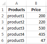
To insert a column between other columns for filling in pricelist items numbering you can use one of the two ways:
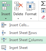
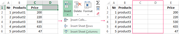
- Move the cursor to activate A1 cell. Then go to tab «HOME», tool section «Cells» and click «Insert», in the popup menu select «Insert Sheet Columns» option.
- Right-click the heading of column A. Select «Insert» option on the shortcut menu.
- Select the column, and press the hotkey combination CTRL+SHIFT+PLUS.
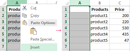
Now you can type the numbers of pricelist line items.
Simultaneous insertion of several columns
The pricelist still lacks two columns: quantity and units (items, kilograms, liters, packs). To add simultaneously, highlight the two-cell range (C1:D1). Then use the same tool on the «Insert»-«Insert Sheet Columns» main tab.
Alternatively, highlight two headings of columns C and D, right-click and select «Insert» option.
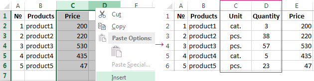
Note. Columns are always added to the left side. There appear as many new columns as many old ones have been highlighted. The order of inserted also depends on the order of highlighting. For example, next but one etc.
How to insert a row between rows in Excel?
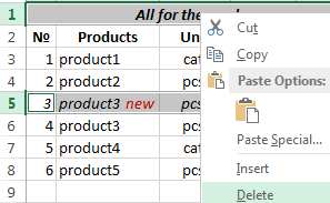
Now let’s add a heading and a new goods line item «All for the garden» to the pricelist. To this end, let’s insert two new rows simultaneously.
Highlight the nonadjacent range of two cells A1,A4 (note that character “,” is used instead of character “:” – it means that two nonadjacent ranges should be highlighted; to make sure, type A1; A4 in the name field and press Enter). You know from the previous tutorials how to highlight nonadjacent ranges.
Now once again use the tool «HOME»-«Insert»-«Insert Sheet Columns». The picture shows how to insert a blank row between other rows in Excel.
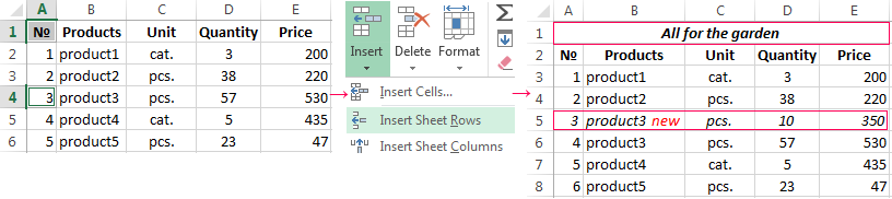
It is easy to guess the second way. You need to highlight headings of rows 1 and 3, right-click on one of the highlighted rows and select «Insert» option.
To add a row or a column in Excel use hot keys CTRL+SHIFT+PLUS having highlighted the appropriate row or column.
Note. New rows are always added above the highlighted rows.
Deleting rows and columns
When working with Excel you need to delete rows and columns as often as to insert them. Therefore, you have to practice.
By way of illustration, let’s delete from our pricelist the numbering of goods line items and the unit column simultaneously.
Highlight the nonadjacent range of cells A1; D1 and select «HOME»-«Delete»-«Delete Sheet Rows». The shortcut menu can also be used for deleting if you highlight headings A1 and D1 instead of cells.
Row deleting is performed in the similar way. You only need to select a tool in the appropriate menu. Applying a shortcut menu is the same. You only have to highlight the rows correspondingly by row numbers.
To delete a row or a column in Excel, use hot keys CTRL+MINUS having preliminary highlighted them.
Note. Inserting new columns and rows is in fact substitution, as the number of rows (1 048 576) and columns (16 384) doesn’t change. The new just replace the old ones. You should consider this fact when filling in the sheet with data by more than 50% — 80%.