
To start a new line of text or add spacing between lines or paragraphs of text in a worksheet cell, press Alt+Enter to insert a line break.
-
Double-click the cell in which you want to insert a line break.
-
Click the location inside the selected cell where you want to break the line.
-
Press Alt+Enter to insert the line break.
To start a new line of text or add spacing between lines or paragraphs of text in a worksheet cell, press CONTROL + OPTION + RETURN to insert a line break.
-
Double-click the cell in which you want to insert a line break.
-
Click the location inside the selected cell where you want to break the line.
-
Press CONTROL+OPTION+RETURN to insert the line break.
To start a new line of text or add spacing between lines or paragraphs of text in a worksheet cell, press Alt+Enter to insert a line break.
-
Double-click the cell in which you want to insert a line break (or select the cell and then press F2).
-
Click the location inside the selected cell where you want to break the line.
-
Press Alt+Enter to insert the line break.
-
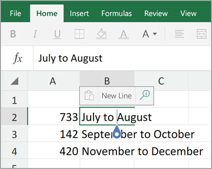
Double-tap within the cell.
-
Tap the place where you want a line break, and then tap the blue cursor.

-
Tap New Line in the contextual menu.
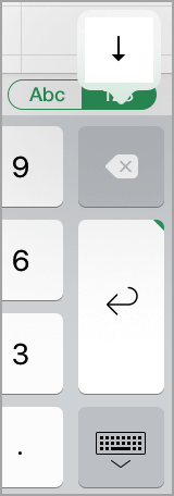
Note: You cannot start a new line of text in Excel for iPhone.
-
Tap the keyboard toggle button to open the numeric keyboard.
-
Press and hold the return key to view the line break key, and then drag your finger to that key.
Excel 2016 Click the location inside the cell where you want to break the line or insert a new line and press Alt+Enter.
Contents
- 1 How do you press enter in Excel and stay in the same cell?
- 2 How do I enter multiple lines in an Excel cell?
- 3 Which command is used to enter a line in a cell in Excel?
- 4 Can’t hit Enter in Excel cell?
- 5 When you press the Enter key the cell pointer?
- 6 How do you press Enter?
- 7 How do you insert multiple lines in one cell?
- 8 How do you show all writing in an Excel cell?
- 9 What is Ctrl Enter in Excel?
- 10 How do you put a dot point in Excel?
- 11 What can I use instead of Enter key?
- 12 How do you press Enter without pressing enter?
- 13 What is shortcut for Enter key?
- 14 When you type data in a cell and press Enter?
- 15 Which commands is used to display text in a cell in multiple lines?
- 16 How do I get cells to show all text in sheets?
- 17 What does Ctrl Alt Enter do?
How do you press enter in Excel and stay in the same cell?
Stay in the same cell after pressing the Enter key with Shortcut Keys. In Excel, you can also use shortcut keys to solve this task. After entering the content, please press Ctrl + Enter keys together instead of just Enter key, and you can see the entered cell is still selected.
How do I enter multiple lines in an Excel cell?
5 steps to better looking data
- Click on the cell where you need to enter multiple lines of text.
- Type the first line.
- Press Alt + Enter to add another line to the cell. Tip.
- Type the next line of text you would like in the cell.
- Press Enter to finish up.
Which command is used to enter a line in a cell in Excel?
To start a new line in an Excel cell, you can use the following keyboard shortcut:
- For Windows – ALT + Enter.
- For Mac – Control + Option + Enter.
Can’t hit Enter in Excel cell?
Cell Movement After Enter
- Display the Excel Options dialog box.
- At the left of the dialog box click Advanced.
- Make sure the After Pressing Enter Move Selection check box is selected.
- Use the Direction drop-down list to specify the direction that Excel should move.
- Click OK.
When you press the Enter key the cell pointer?
By default, in Microsoft Excel, when you press the Enter key, it moves the cell pointer one cell down.
How do you press Enter?
Alternatively known as a Return key, with a keyboard, the Enter key sends the cursor to the beginning of the next line or executes a command or operation. Most full-sized PC keyboards have two Enter keys; one above the right Shift key and another on the bottom right of the numeric keypad.
How do you insert multiple lines in one cell?
If you want to paste all the contents into one cell, you can use this method.
- Press the shortcut key “Ctrl + C” on the keyboard.
- And then switch to the Excel worksheet.
- Now double click the target cell in the worksheet.
- After that, press the shortcut key “Ctrl + V” on the keyboard.
How do you show all writing in an Excel cell?
Select the cells that you want to display all contents, and click Home > Wrap Text. Then the selected cells will be expanded to show all contents.
What is Ctrl Enter in Excel?
#2 – Ctrl+Enter to Fill All Selected Cells with the Same Data or Formula. When we are entering data or a formula in a cell, and have multiple cells selected, Ctrl+Enter will copy the data/formula to all of the selected cells.
How do you put a dot point in Excel?
How to Add Bullet Points in Excel
- Select the cell in which you want to insert the bullet.
- Either double click on the cell or press F2 – to get into edit mode.
- Hold the ALT key, press 7 or 9, leave the ALT key.
- As soon as you leave the ALT key, a bullet would appear.
What can I use instead of Enter key?
You could replace it or use Ctrl+M instead of enter key. If the Enter key is not working, there is a high chance the Enter key is fine, but some other key is stuck, most likely ALT, CTRL, SHIFT, DEL, any key that would not show up doing something immediately.
How do you press Enter without pressing enter?
You can use CTRL + J or CTRL + M as an alternative to Enter .
What is shortcut for Enter key?
Windows Laptops:
Hold down the “fn” key and press the ‘num lk’ key. On some laptops this key is the same as the ‘end’ key. Once the num lock function has been enabled, the Return key will function as an Enter key.
When you type data in a cell and press Enter?
By default when typing data or a formula into a cell and pressing enter, the active cell cursor will move down one cell. You don’t have to be stuck with this if you don’t want it though. You can also have it go up, left, right or not move at all if you want.
Which commands is used to display text in a cell in multiple lines?
You can put multiple lines in a cell with pressing Alt + Enter keys simultaneously while entering texts. Pressing the Alt + Enter keys simultaneously helps you separate texts with different lines in one cell.
How do I get cells to show all text in sheets?
How to Wrap Text in Google Sheets
- Select the cells you want to set to wrap.
- Click Format.
- Select Text wrapping.
- Select Wrap.
What does Ctrl Alt Enter do?
Popular programs using this shortcut
You can apply different paragraph styles to the left and right of the style separator. That can be useful for references. And you can also use it to limit the text that is included in the Table of Contents. PyCharm 2018.2 – Start a new line before the current one.

Как известно, по умолчанию в одной ячейке листа Excel располагается одна строка с числами, текстом или другими данными. Но, что делать, если нужно перенести текст в пределах одной ячейки на другую строку? Данную задачу можно выполнить, воспользовавшись некоторыми возможностями программы. Давайте разберемся, как сделать перевод строки в ячейке в Excel.
Способы переноса текста
Некоторые пользователи пытаются перенести текст внутри ячейки нажатием на клавиатуре кнопки Enter. Но этим они добиваются только того, что курсор перемещается на следующую строку листа. Мы же рассмотрим варианты переноса именно внутри ячейки, как очень простые, так и более сложные.
Способ 1: использование клавиатуры
Самый простой вариант переноса на другую строку, это установить курсор перед тем отрезком, который нужно перенести, а затем набрать на клавиатуре сочетание клавиш Alt+Enter.
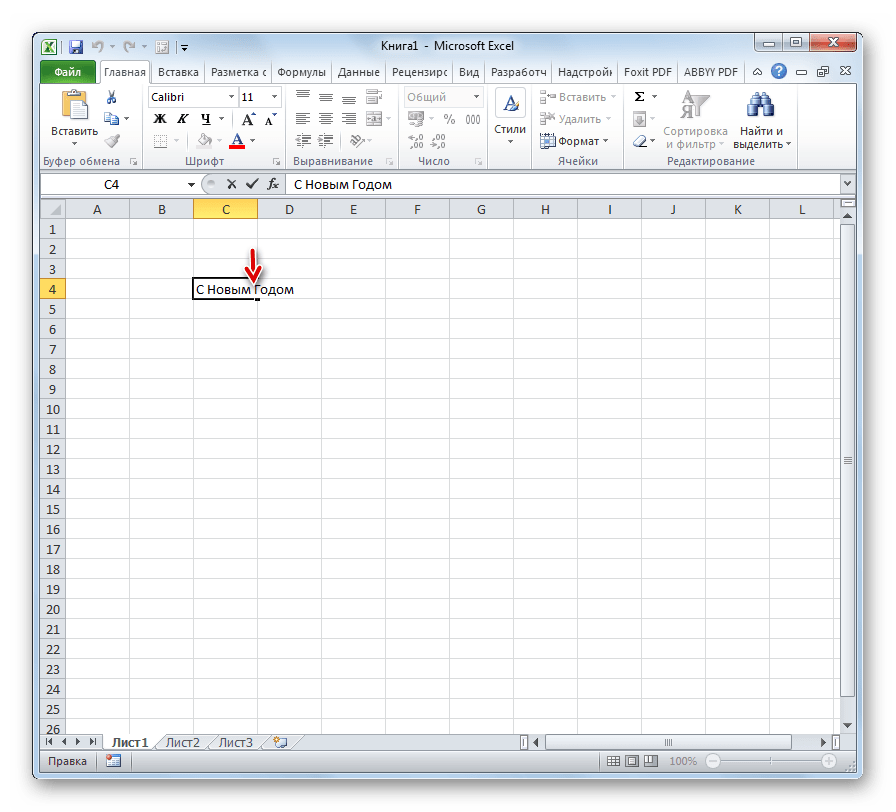
В отличие от использования только одной кнопки Enter, с помощью этого способа будет достигнут именно такой результат, который ставится.
Способ 2: форматирование
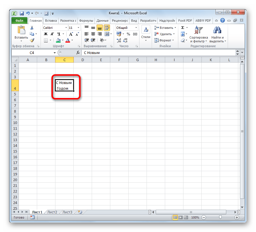
Если перед пользователем не ставится задачи перенести на новую строку строго определенные слова, а нужно только уместить их в пределах одной ячейки, не выходя за её границы, то можно воспользоваться инструментом форматирования.
-
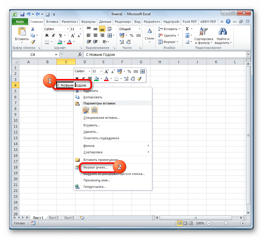
Выделяем ячейку, в которой текст выходит за пределы границ. Кликаем по ней правой кнопкой мыши. В открывшемся списке выбираем пункт «Формат ячеек…».
После этого, если данные будут выступать за границы ячейки, то она автоматически расширится в высоту, а слова станут переноситься. Иногда приходится расширять границы вручную.
Чтобы подобным образом не форматировать каждый отдельный элемент, можно сразу выделить целую область. Недостаток данного варианта заключается в том, что перенос выполняется только в том случае, если слова не будут вмещаться в границы, к тому же разбитие осуществляется автоматически без учета желания пользователя.
Способ 3: использование формулы
Также можно осуществить перенос внутри ячейки при помощи формул. Этот вариант особенно актуален в том случае, если содержимое выводится с помощью функций, но его можно применять и в обычных случаях.
- Отформатируйте ячейку, как указано в предыдущем варианте.
- Выделите ячейку и введите в неё или в строку формул следующее выражение:
Вместо элементов «ТЕКСТ1» и «ТЕКСТ2» нужно подставить слова или наборы слов, которые хотите перенести. Остальные символы формулы изменять не нужно.
Главным недостатком данного способа является тот факт, что он сложнее в выполнении, чем предыдущие варианты.
В целом пользователь должен сам решить, каким из предложенных способов оптимальнее воспользоваться в конкретном случае. Если вы хотите только, чтобы все символы вмещались в границы ячейки, то просто отформатируйте её нужным образом, а лучше всего отформатировать весь диапазон. Если вы хотите устроить перенос конкретных слов, то наберите соответствующее сочетание клавиш, как рассказано в описании первого способа. Третий вариант рекомендуется использовать только тогда, когда данные подтягиваются из других диапазонов с помощью формулы. В остальных случаях использование данного способа является нерациональным, так как имеются гораздо более простые варианты решения поставленной задачи.
Отблагодарите автора, поделитесь статьей в социальных сетях.

Довольно часто возникает вопрос, как сделать перенос на другую строку внутри ячейки в Экселе? Этот вопрос возникает когда текст в ячейке слишком длинный, либо перенос необходим для структуризации данных. В таком случае бывает не удобно работать с таблицами. Обычно перенос текста осуществляется с помощью клавиши Enter. Например, в программе Microsoft Office Word. Но в Microsoft Office Excel при нажатии на Enter мы попадаем на соседнюю нижнюю ячейку.
Итак нам требуется осуществить перенос текста на другую строку. Для переноса нужно нажать сочетание клавиш Alt+Enter. После чего слово, находящееся с правой стороны от курсора перенесется на следующую строку.

Автоматический перенос текста в Excel
В Экселе на вкладке Главная в группе Выравнивание есть кнопка «Перенос текста». Если выделить ячейку и нажать эту кнопку, то текст в ячейке будет переноситься на новую строку автоматически в зависимости от ширины ячейки. Для автоматического переноса требуется выполнить простое нажатие кнопки.

Убрать перенос с помощью функции и символа переноса
Для того, что бы убрать перенос мы можем использовать функцию ПОДСТАВИТЬ.
Функция заменяет один текст на другой в указанной ячейке. В нашем случае мы будем заменять символ пробел на символ переноса.
=ПОДСТАВИТЬ (текст;стар_текст;нов_текст;[номер вхождения])
Итоговый вид формулы:
- А1 – ячейка содержащая текст с переносами,
- СИМВОЛ(10) – символ переноса строки,
- » » – пробел.

Если же нам наоборот требуется вставить символ переноса на другую строку, вместо пробела проделаем данную операцию наоборот.
Что бы функция работало корректно во вкладке Выравнивание (Формат ячеек) должен быть установлен флажок «Переносить по словам».
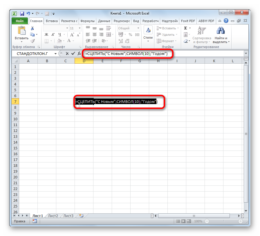
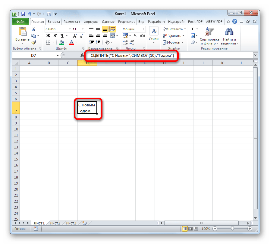
Перенос с использование формулы СЦЕПИТЬ
Для решения нашей проблемы можно использовать формулу СЦЕПИТЬ.
У нас имеется текст в ячейках A1 и B1. Введем в B3 следующую формулу:

Как в примере, который я приводил выше, для корректной работы функции в свойствах требуется установить флажок «переносить по словам».
Часто требуется внутри одной ячейки Excel сделать перенос текста на новую строку. То есть переместить текст по строкам внутри одной ячейки как указано на картинке. Если после ввода первой части текста просто нажать на клавишу ENTER, то курсор будет перенесен на следующую строку, но другую ячейку, а нам требуется перенос в этой же ячейке.

Это очень частая задача и решается она очень просто — для переноса текста на новую строку внутри одной ячейки Excel необходимо нажать ALT+ENTER (зажимаете клавишу ALT, затем не отпуская ее, нажимаете клавишу ENTER)
Как перенести текст на новую строку в Excel с помощью формулы
Иногда требуется сделать перенос строки не разово, а с помощью функций в Excel. Вот как в этом примере на рисунке. Мы вводим имя, фамилию и отчество и оно автоматически собирается в ячейке A6

Для начала нам необходимо сцепить текст в ячейках A1 и B1 ( A1&B1 ), A2 и B2 ( A2&B2 ), A3 и B3 ( A3&B3 )
После этого объединим все эти пары, но так же нам необходимо между этими парами поставить символ (код) переноса строки. Есть специальная таблица знаков (таблица есть в конце данной статьи), которые можно вывести в Excel с помощью специальной функции СИМВОЛ(число), где число это число от 1 до 255, определяющее определенный знак.
Например, если прописать =СИМВОЛ(169), то мы получим знак копирайта ©
Нам же требуется знак переноса строки, он соответствует порядковому номеру 10 — это надо запомнить.
Код (символ) переноса строки — 10
Следовательно перенос строки в Excel в виде функции будет выглядеть вот так СИМВОЛ(10)
Примечание: В VBA Excel перенос строки вводится с помощью функции Chr и выглядит как Chr (10)
Итак, в ячейке A6 пропишем формулу
= A1&B1 &СИМВОЛ(10)& A2&B2 &СИМВОЛ(10)& A3&B3
В итоге мы должны получить нужный нам результат.
Обратите внимание! Чтобы перенос строки корректно отображался необходимо включить «перенос по строкам» в свойствах ячейки.
Для этого выделите нужную нам ячейку (ячейки), нажмите на правую кнопку мыши и выберите «Формат ячеек. » 
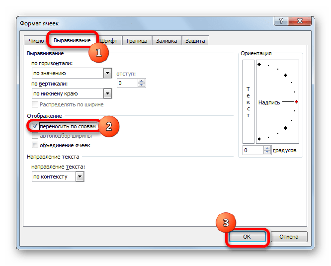
В открывшемся окне во вкладке «Выравнивание» необходимо поставить галочку напротив «Переносить по словам» как указано на картинке, иначе перенос строк в Excel не будет корректно отображаться с помощью формул.

Как в Excel заменить знак переноса на другой символ и обратно с помощью формулы
Можно поменять символ перенос на любой другой знак, например на пробел, с помощью текстовой функции ПОДСТАВИТЬ в Excel

Рассмотрим на примере, что на картинке выше. Итак, в ячейке B1 прописываем функцию ПОДСТАВИТЬ:
A1 — это наш текст с переносом строки;
СИМВОЛ(10) — это перенос строки (мы рассматривали это чуть выше в данной статье);
» » — это пробел, так как мы меняем перенос строки на пробел
Если нужно проделать обратную операцию — поменять пробел на знак (символ) переноса, то функция будет выглядеть соответственно:
Напоминаю, чтобы перенос строк правильно отражался, необходимо в свойствах ячеек, в разделе «Выравнивание» указать «Переносить по строкам».
Как поменять знак переноса на пробел и обратно в Excel с помощью ПОИСК — ЗАМЕНА
Бывают случаи, когда формулы использовать неудобно и требуется сделать замену быстро. Для этого воспользуемся Поиском и Заменой. Выделяем наш текст и нажимаем CTRL+H, появится следующее окно.

Если нам необходимо поменять перенос строки на пробел, то в строке «Найти» необходимо ввести перенос строки, для этого встаньте в поле «Найти», затем нажмите на клавишу ALT , не отпуская ее наберите на клавиатуре 010 — это код переноса строки, он не будет виден в данном поле.
После этого в поле «Заменить на» введите пробел или любой другой символ на который вам необходимо поменять и нажмите «Заменить» или «Заменить все».
Кстати, в Word это реализовано более наглядно.
Если вам необходимо поменять символ переноса строки на пробел, то в поле «Найти» вам необходимо указать специальный код «Разрыва строки», который обозначается как ^l
В поле «Заменить на: » необходимо сделать просто пробел и нажать на «Заменить» или «Заменить все».

Вы можете менять не только перенос строки, но и другие специальные символы, чтобы получить их соответствующий код, необходимо нажать на кнопку «Больше >> «, «Специальные» и выбрать необходимый вам код. Напоминаю, что данная функция есть только в Word, в Excel эти символы не будут работать.

Как поменять перенос строки на пробел или наоборот в Excel с помощью VBA
Рассмотрим пример для выделенных ячеек. То есть мы выделяем требуемые ячейки и запускаем макрос
1. Меняем пробелы на переносы в выделенных ячейках с помощью VBA
Sub ПробелыНаПереносы()
For Each cell In Selection
cell.Value = Replace (cell.Value, Chr (32) , Chr (10) )
Next
End Sub
2. Меняем переносы на пробелы в выделенных ячейках с помощью VBA
Sub ПереносыНаПробелы()
For Each cell In Selection
cell.Value = Replace (cell.Value, Chr (10) , Chr (32) )
Next
End Sub
Код очень простой Chr (10) — это перенос строки, Chr (32) — это пробел. Если требуется поменять на любой другой символ, то заменяете просто номер кода, соответствующий требуемому символу.
Коды символов для Excel
Ниже на картинке обозначены различные символы и соответствующие им коды, несколько столбцов — это различный шрифт. Для увеличения изображения, кликните по картинке.
Содержание
- Start a new line of text inside a cell in Excel
- Need more help?
- How To Press Enter In An Excel Cell?
- How do you press enter in Excel and stay in the same cell?
- How do I enter multiple lines in an Excel cell?
- Which command is used to enter a line in a cell in Excel?
- Can’t hit Enter in Excel cell?
- When you press the Enter key the cell pointer?
- How do you press Enter?
- How do you insert multiple lines in one cell?
- How do you show all writing in an Excel cell?
- What is Ctrl Enter in Excel?
- How do you put a dot point in Excel?
- What can I use instead of Enter key?
- How do you press Enter without pressing enter?
- What is shortcut for Enter key?
- When you type data in a cell and press Enter?
- Which commands is used to display text in a cell in multiple lines?
- How do I get cells to show all text in sheets?
- What does Ctrl Alt Enter do?
- How to Start a New Line in Excel Cell (Keyboard Shortcut + Formula)
- Start a New Line in Excel Cell – Keyboard Shortcut
- Start a New Line in Excel Cell Using Formula
- Using TextJoin Formula
- Using Concatenate Formula
- New Line in an Excel Cell
- Insert a New Line in an Excel Cell
- Top 3 Ways to Insert a New Line in a Cell of Excel
- #1 – Using the Shortcut Keys “Alt+Enter”
- #2–Using the “CHAR(10)” Formula of Excel
- #3–Using the Named Formula [CHAR(10)]
- Frequently Asked Questions
- Recommended Articles
Start a new line of text inside a cell in Excel
To start a new line of text or add spacing between lines or paragraphs of text in a worksheet cell, press Alt+Enter to insert a line break.
Double-click the cell in which you want to insert a line break.
Click the location inside the selected cell where you want to break the line.
Press Alt+Enter to insert the line break.
To start a new line of text or add spacing between lines or paragraphs of text in a worksheet cell, press CONTROL + OPTION + RETURN to insert a line break.
Double-click the cell in which you want to insert a line break.
Click the location inside the selected cell where you want to break the line.
Press CONTROL+OPTION+RETURN to insert the line break.
To start a new line of text or add spacing between lines or paragraphs of text in a worksheet cell, press Alt+Enter to insert a line break.
Double-click the cell in which you want to insert a line break (or select the cell and then press F2).
Click the location inside the selected cell where you want to break the line.
Press Alt+Enter to insert the line break.
Double-tap within the cell.
Tap the place where you want a line break, and then tap the blue cursor.

Tap New Line in the contextual menu.
Note: You cannot start a new line of text in Excel for iPhone.
Tap the keyboard toggle button to open the numeric keyboard.

Press and hold the return key to view the line break key, and then drag your finger to that key.
Need more help?
You can always ask an expert in the Excel Tech Community or get support in the Answers community.
Источник
How To Press Enter In An Excel Cell?
Excel 2016 Click the location inside the cell where you want to break the line or insert a new line and press Alt+Enter.
How do you press enter in Excel and stay in the same cell?
Stay in the same cell after pressing the Enter key with Shortcut Keys. In Excel, you can also use shortcut keys to solve this task. After entering the content, please press Ctrl + Enter keys together instead of just Enter key, and you can see the entered cell is still selected.
How do I enter multiple lines in an Excel cell?
5 steps to better looking data
- Click on the cell where you need to enter multiple lines of text.
- Type the first line.
- Press Alt + Enter to add another line to the cell. Tip.
- Type the next line of text you would like in the cell.
- Press Enter to finish up.
Which command is used to enter a line in a cell in Excel?
To start a new line in an Excel cell, you can use the following keyboard shortcut:
- For Windows – ALT + Enter.
- For Mac – Control + Option + Enter.
Can’t hit Enter in Excel cell?
Cell Movement After Enter
- Display the Excel Options dialog box.
- At the left of the dialog box click Advanced.
- Make sure the After Pressing Enter Move Selection check box is selected.
- Use the Direction drop-down list to specify the direction that Excel should move.
- Click OK.
When you press the Enter key the cell pointer?
By default, in Microsoft Excel, when you press the Enter key, it moves the cell pointer one cell down.
How do you press Enter?
Alternatively known as a Return key, with a keyboard, the Enter key sends the cursor to the beginning of the next line or executes a command or operation. Most full-sized PC keyboards have two Enter keys; one above the right Shift key and another on the bottom right of the numeric keypad.
How do you insert multiple lines in one cell?
If you want to paste all the contents into one cell, you can use this method.
- Press the shortcut key “Ctrl + C” on the keyboard.
- And then switch to the Excel worksheet.
- Now double click the target cell in the worksheet.
- After that, press the shortcut key “Ctrl + V” on the keyboard.
How do you show all writing in an Excel cell?
Select the cells that you want to display all contents, and click Home > Wrap Text. Then the selected cells will be expanded to show all contents.
What is Ctrl Enter in Excel?
#2 – Ctrl+Enter to Fill All Selected Cells with the Same Data or Formula. When we are entering data or a formula in a cell, and have multiple cells selected, Ctrl+Enter will copy the data/formula to all of the selected cells.
How do you put a dot point in Excel?
How to Add Bullet Points in Excel
- Select the cell in which you want to insert the bullet.
- Either double click on the cell or press F2 – to get into edit mode.
- Hold the ALT key, press 7 or 9, leave the ALT key.
- As soon as you leave the ALT key, a bullet would appear.
What can I use instead of Enter key?
You could replace it or use Ctrl+M instead of enter key. If the Enter key is not working, there is a high chance the Enter key is fine, but some other key is stuck, most likely ALT, CTRL, SHIFT, DEL, any key that would not show up doing something immediately.
How do you press Enter without pressing enter?
You can use CTRL + J or CTRL + M as an alternative to Enter .
What is shortcut for Enter key?
Windows Laptops:
Hold down the “fn” key and press the ‘num lk’ key. On some laptops this key is the same as the ‘end’ key. Once the num lock function has been enabled, the Return key will function as an Enter key.
When you type data in a cell and press Enter?
By default when typing data or a formula into a cell and pressing enter, the active cell cursor will move down one cell. You don’t have to be stuck with this if you don’t want it though. You can also have it go up, left, right or not move at all if you want.
Which commands is used to display text in a cell in multiple lines?
You can put multiple lines in a cell with pressing Alt + Enter keys simultaneously while entering texts. Pressing the Alt + Enter keys simultaneously helps you separate texts with different lines in one cell.
How do I get cells to show all text in sheets?
How to Wrap Text in Google Sheets
- Select the cells you want to set to wrap.
- Click Format.
- Select Text wrapping.
- Select Wrap.
What does Ctrl Alt Enter do?
Popular programs using this shortcut
You can apply different paragraph styles to the left and right of the style separator. That can be useful for references. And you can also use it to limit the text that is included in the Table of Contents. PyCharm 2018.2 – Start a new line before the current one.
Источник
How to Start a New Line in Excel Cell (Keyboard Shortcut + Formula)
Watch Video – Start a New Line in a Cell in Excel (Shortcut + Formula)
In this Excel tutorial, I will show you how to start a new line in an Excel cell.
You can start a new line in the same cell in Excel by using:
- A keyboard shortcut to manually force a line break.
- A formula to automatically enter a line break and force part of the text to start a new line in the same cell.
This Tutorial Covers:
Start a New Line in Excel Cell – Keyboard Shortcut
To start a new line in an Excel cell, you can use the following keyboard shortcut:
- For Windows – ALT + Enter.
- For Mac – Control + Option + Enter.
Here are the steps to start a new line in Excel Cell using the shortcut ALT + ENTER:
- Double click on the cell where you want to insert the line break (or press F2 key to get into the edit mode).
- Place the cursor where you want to insert the line break.
- Hold the ALT key and press the Enter key for Windows (for Mac – hold the Control and Option keys and hit the Enter key).

Start a New Line in Excel Cell Using Formula
While keyboard shortcut is fine when you are manually entering data and need a few line breaks.
But in case you need to combine cells and get a line break while combining these cells, you can use a formula to do this.
Using TextJoin Formula
If you’re using Excel 2019 or Office 365 (Windows or Mac), you can use the TEXTJOIN function to combine cells and insert a line break in the resulting data.
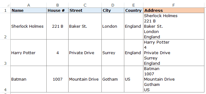
For example, suppose we have a dataset as shown below and you want to combine these cells to get the name and the address in the same cell (with each part in a separate line):

The following formula will do this:
At first, you may see the result as one single line that combines all the address parts (as shown below).

To make sure you have all the line breaks in between each part, make sure the wrap text feature is enabled.
To enable Wrap text, select the cells with the results, click on the Home tab, and within the alignment group, click on the ‘Wrap Text’ option.

Once you click on the Wrap Text option, you will see the resulting data as shown below (with each address element in a new line):

Using Concatenate Formula
If you’re using Excel 2016 or prior versions, you won’t have the TEXTJOIN formula available.
So you can use the good old CONCATENATE function (or the ampersand & character) to combine cells and get line break in between.
Again, considering you have the dataset as shown below that you want to combine and get a line break in between each cell:
For example, if I combine using the text in these cells using an ampersand (&), I would get something as shown below:

While this combines the text, this is not really the format that I want. You can try using the text wrap, but that wouldn’t work either.
If I am creating a mailing address out of this, I need the text from each cell to be in a new line in the same cell.
To insert a line break in this formula result, we need to use CHAR(10) along with the above formula.
CHAR(10) is a line feed in Windows, which means that it forces anything after it to go to a new line.
So to do this, use the below formula:
This formula would enter a line break in the formula result and you would see something as shown below:
IMPORTANT : For this to work, you need to wrap text in excel cells. To wrap text, go to Home –> Alignment –> Wrap Text. It is a toggle button.

Tip: If you are using MAC, use CHAR(13) instead of CHAR(10).
You may also like the following Excel Tutorial:
Источник
New Line in an Excel Cell


Insert a New Line in an Excel Cell
A new line in excel cell is inserted when one needs to move a string to the next line of the cell. To insert a new line, a line break must be added at the relevant place. A line break tells Excel to break the existing line and begin a new line (within the same cell) with the immediately following character. When line breaks are inserted in a cell, its content can be seen in multiple lines.
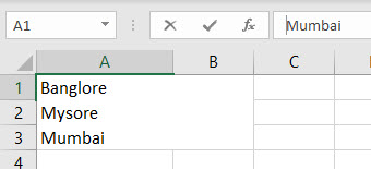
For example, in the following image, a line break has been inserted after the cities Bangalore and Mysore. So, a total of two line breaks have been inserted in cell A1. Notice that the three cities are in three different rows of the same cell.

Starting a new line in an excel cell ensures that the lengthy text strings are split into multiple lines. This improves the readability and lends a neat look to the worksheet. To obtain the right result after inserting line breaks, ensure that the wrap text feature of Excel is turned on.
Table of contents
Top 3 Ways to Insert a New Line in a Cell of Excel
The methods to start a new line in a cell of Excel are listed as follows:
- Shortcut keys “Alt+Enter”
- “CHAR(10)” formula of Excel
- Named formula [CHAR(10)]
Let us consider an example of each technique.
Note: The line feed (LF) and carriage return Carriage Return Carriage Return in excel cell is a way to shift to a new line within the same cell. This could be treated as a line breaker which fits in huge data in an organized manner within one cell. read more (CR) are two terms closely related to a line break. The LF moves the cursor to the next line within the cell. In contrast, a CR moves the cursor to the beginning (or the first position) of the same line. So, with a CR alone, the cursor does not move to the next line.
Every operating system considers a line break (LF or CR or a combination of CR and LF) differently. For instance, when a line break is inserted in the Windows operating system, both CR and LF (called CR+LF or CRLF) are inserted together.
The CRLF moves the cursor to the beginning of the next line. However, the “Alt+Enter” method inserts only line feeds in Excel. The ASCII (American Standard Code for Information Interchange) codes for LF and CR are 10 and 13 respectively.
In this article, the usage of code 10 has been shown in example #2. Further, this article uses the term line break in place of line feed and carriage return. Hence, consider all three (line break, line feed, and carriage return) to be the same in this article.
#1 – Using the Shortcut Keys “Alt+Enter”
The following image shows the names of three cities of India in cell A1. We want to insert a line break after the first two cities of this cell. Use the keys “Alt+Enter” of Excel.

The steps to insert line breaks by using the keys “Alt+Enter” are listed as follows:
Step 1: Double-click inside cell A1. Next, move and bring the cursor immediately before the “M” of Mysore. To do this, either move the cursor with the arrow keys of the keyboard or click at the stated position with the left-click of the mouse.
The cursor is placed before Mysore because a line break needs to be inserted at this position.
Note: Alternatively, one can also place the cursor at the stated position in the formula bar.

Step 2: Press the keys “Alt+Enter.” For this shortcut to work, hold the “Alt” key while pressing the “Enter” key.
A new line is inserted before “Mysore,” as shown in the following image.

Step 3: Place the cursor before the “M” of Mumbai by using the left-click of the mouse. Press the keys “Alt+Enter,” the way they were pressed in the preceding step.
The name “Mumbai” shifts to a new line within the same cell of Excel. This is shown in the following image.
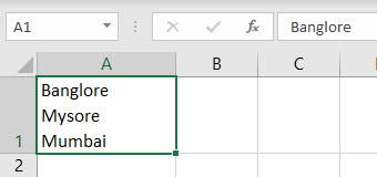
Step 4: Press the “Enter” key to exit the Edit mode. The following image shows the names of the three cities in multiple lines of a single cell (cell A1) of Excel. This result will be displayed only if the wrap text feature of Excel is turned on.
Notice that the formula bar (in the following image) shows a line break after Bangalore.
Note: The “wrap text” is a toggle button in the “alignment” group of the Home tab. It can also be accessed from the “alignment” tab of the “format cells” window. This window can be opened by pressing the shortcut “Ctrl+1.”
By default, the wrap text feature is turned on when a line break is inserted with the “Alt+Enter” method in Excel. To cross-check, keep cell A1 selected and notice that the “wrap text” button is automatically activated after inserting a line break with the shortcut keys.
If the wrap text button is turned off, the content of cell A1 will display in a single line. However, the line breaks will still be visible in the formula bar.
#2–Using the “CHAR(10)” Formula of Excel
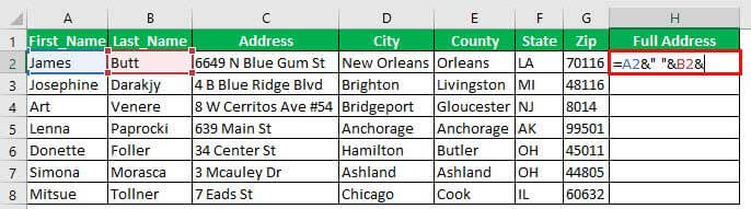
The following image shows the names and addresses of some people. The first and the last names have been split into columns A and B respectively. The address has been split into columns C to G. We want to perform the following tasks:
- Join the first and the last name to the full address of each person. For this, combine the strings of columns A and B with those of columns C to G. Use the ampersand (&) to join the stated strings. Ensure that a single space character precedes each string of the address.
- Insert a line break between the last name and the first character of the address. Use the CHAR function for inserting line breaks.
In the end, the complete name should be in one line, followed by the address in the subsequent lines of the cell. Further, use a single formula for performing the given tasks. Explain the formula used.
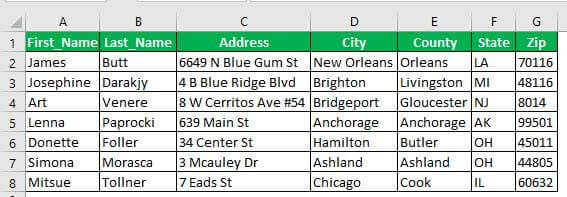
Step 1: Insert a new column to the right of the given dataset. We have inserted column H titled “full address.” This is shown in the following image.

Step 2: Begin by combining the first and last names (of row 2) with the ampersand. To do this, type the following formula in cell H2.
This formula joins the first and the last names of cells A2 and B2 and also inserts a space between them. However, the formula is currently incomplete.
Step 3: Extend the preceding formula to include the CHAR function. Open this function by typing “CHAR,” followed by the opening parenthesis.
The opening of the CHAR function is shown in the following image.
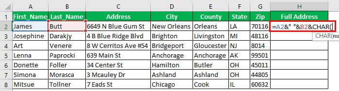
Step 4: Insert the number 10 within the CHAR function. The “CHAR(10)” formula inserts a line break in Excel.
Note: The syntax of the CHAR function is “CHAR(number).” This function returns a character when a number between 1 and 255 is entered. The character is returned from the character set of the user’s computer.
Earlier, the Windows operating system used the ASCII and the ANSI character sets, which have now been replaced by Unicode. The ASCII stands for American Standard Code for Information Interchange. The ANSI character set was created by the American National Standard Institute.
In contrast, the Macintosh operating system uses the Macintosh character set. So, the Macintosh users may use the formula “CHAR(13)” to insert a line break in Excel.
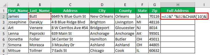
Step 5: Insert the cell references to be joined with the strings of cells A2 and B2. So, in cell H2, enter the following formula by excluding the beginning and ending double quotation marks.
Press the “Enter” key. The output appears in cell H2. The formula and the output are shown in the following image. The output is not fully visible as it is in a single line of cell H2 of Excel.

Explanation of the formula: The preceding formula joins the first and the last names (in cells A2 and B2) with the entire address of a person (in cells D2, E2, F2, and G2). The ampersand (&) is used to join.
Notice that, in the formula, a space character has been inserted preceding the strings of cells D2, E2, F2, and G2. This space character is inserted within double quotation marks (like “ ”). These spaces of the formula ensure that spaces are inserted as separators in the output. Moreover, the separators are inserted at exactly those places (in the output) where they have been entered in the formula.
However, no space is inserted between the strings of cells B2 and C2. Rather, the “CHAR(10)” has been used in place of a space. This is because the “CHAR(10)” moves the immediately following string (of cell C2) to the next line.
Step 6: Activate the wrap text feature of Excel to see the entire content of cell H2. So, select cell H2 and click the “wrap text” button in the “alignment” group of the Home tab.
The output is shown in the following image. The full name and the complete address are visible in cell H2. Not only the strings of cells A2 to G2 have been joined, but a line break has also been inserted after the name (James Butt). As a result, a legible output has been obtained in cell H2.
Note: When a line break is inserted by the CHAR function, the wrap text feature of Excel is not turned on by default. Rather, this feature needs to be enabled manually to see the impact of the line break.

Step 7: Drag the formula of cell H2 till cell H8 by using the fill handle. The fill handle is displayed at the bottom-right corner of cell H2.
The dragging of the fill handle and the outputs are shown in the following image. Hence, the names and addresses have been consolidated neatly in column H.
#3–Using the Named Formula [CHAR(10)]
Working on the dataset of example #2, we want to perform the following tasks:
- Assign the name “NL” to the “CHAR(10)” formula. By doing this, “CHAR(10)” becomes a named formula.
- Add the comment “new line inserter” to the name “NL.”
- Show how to use the name “NL” (representing the named formula) in the ampersand and CHAR formula of example #2. Explain the formula thus used.
Use the “define name” property of Excel for the first two bullet points.
The steps to perform the given tasks by using the named formula are listed as follows:
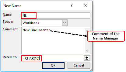
Step 1: Click “define name” from the “defined names” group of the Formulas tab. This option is shown in the following image.
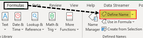
Step 2: The “new name” window opens, as shown in the following image. Make the following insertions in this window:
- In the “name” box, enter the name “NL.”
- In the “scope” box, let the option “workbook” remain selected.
- In the “comment” box, enter the string “new line inserter.”
- In the “refers to” box, enter the formula “=CHAR(10).”
Ensure that the insertions of points “a,” “c,” and “d” are entered without the beginning and ending double quotation marks. Click “Ok” once the insertions are done.
Note 1: The name and the comment cannot exceed 255 characters in length. The name must begin with a letter, underscore (_) or backslash (). Further, the name should not consist of any space characters.
Step 3: Use “NL” in place of “CHAR(10)” in the following formula.
Press the “Enter” key. The outputs are shown in the following image.
Note: When the “N” of “NL” is typed in the formula, Excel shows the name (NL) as well as the comment (new line inserter) in a list of suggestions. To select “NL” from this list, just double-click it.

Explanation of the formula: The outputs of the preceding formula are the same as that of example #2 (in step 7). This is because other than the name “NL,” the formulas of the two examples (examples #2 and #3) are the same.
Since “CHAR(10)” has been named “NL,” we have used this name in the formula instead of the CHAR function. The “wrap text” feature has also been applied to cell H2. This is the reason its content has fitted into multiple lines of cell H2 of Excel.
Notice that using a different name for “CHAR(10)” has not impacted the result. Rather, using the name “NL” has made the preceding formula compact and understandable.
Note: In this example, “CHAR(10)” is considered a named formula. A named formula is one that has been assigned a name in Excel. Assigning a name (like “NL”) to a formula [like “CHAR(10)”] helps refer to the formula by its name.
So, every time one needs to use “CHAR(10)” in the formulas of the current workbook, one can use “NL” in its place. This is because the “scope” in the “new name” window has been set as “workbook.”
Frequently Asked Questions
Inserting a new line means moving the content of a cell to the next line. This allows one to break lengthy text strings and display their data in multiple lines of a single cell. The shortcuts for inserting a line break in Excel are stated as follows:
Windows operating system – The shortcut is “Alt+Enter.” For this shortcut to work, hold the “Alt” key while pressing the “Enter” key.
Macintosh operating system – The shortcut is “Control+Option+Return” (or “Control+Command+Return”). For this shortcut to work, hold the “Control” and the “Option” keys while pressing the “Return” key.
Note: Before using the preceding shortcuts, ensure that the cursor is placed where a line break needs to be inserted.
The CONCATENATE function joins the values of different cells in a single cell. Thereafter, the “CHAR(10)” inserts line breaks in the single output cell.
The CONCATENATE and CHAR formula for inserting a new line in Excel is stated as follows:
“CONCATENATE(cell1,CHAR(10),cell2,CHAR(10),cell3,CHAR(10)…)”
The steps for inserting a new line with the Find and Replace feature of Excel are listed as follows:
a. Select the cells in which a new line needs to be inserted.
b. Press the keys “Ctrl+H” to open the Replace tab of the Find and Replace window. Alternatively, click the “find & select” drop-down from the “editing” group of the Home tab. Then, select the “replace” option.
c. In the “find what” box, type the separator that separates the strings. For instance, if a comma separates the strings, type a comma. Likewise, if a space separates the strings, type a space.
d. In the “replace with” box, press the keys “Ctrl+J.” A small, blinking dot appears in this box.
e. Click “replace all.”
In the selected cells, all occurrences of the separator (typed in step “c”) will be replaced by line breaks.
Note: Use the Find and Replace feature for inserting line breaks when each selected cell contains at least one occurrence of the separator. At the same time, there is a need to replace all these occurrences with line breaks.
The formula to remove a line break from a cell is stated as follows:
“=SUBSTITUTE(cell1,CHAR(10),””)”
The formula to insert a comma in place of a line break is stated as follows:
“=SUBSTITUTE(cell1,CHAR(10),”,”)”
In both the preceding formulas, “cell1” is the cell that contains the string with line breaks. Further, the SUBSTITUTE function replaces every occurrence of “CHAR(10)” with a blank (“”) or a comma (“,”).
Note: Alternatively, the line breaks can be removed with the Find and Replace feature. Press the keys “Ctrl+J” in the “find what” box. In the “replace with” box, type a separator (like a space or comma) that needs to be inserted in place of a line break. Click “replace all” at the end.
Since removing line breaks with the Find and Replace feature may not always work as desired, one can use the preceding SUBSTITUTE and CHAR formulas.
Recommended Articles
This has been a guide to inserting a new line in a cell of Excel. Here we learn how to start a new line in an Excel cell by using the shortcut keys (Alt+Enter), CHAR function, and named formula [CHAR(10)]. A downloadable template is available on the website. You may learn more about Excel from the following articles–
Источник
Перейти к содержимому
Одним из наиболее популярных вопросов среди пользователей программы «Эксель» является вопрос о том, каким образом перенести текст внутри ячейки на новую строку нажатием клавиши ENTER, чтобы активная ячейка не менялась и не перескакивала ниже.
Так, например, если Вам нужно написать текст в форме списка, чтобы каждое предложение начиналось с новой строки, многие пользователи выходят из затруднительного положения при помощи следующей хитрости:
набирают текст в программе Word или ином редакторе текстовых документов, потом копируют и вставляют уже форматированный текст в ячейку Excel.
Описанная процедура довольно трудоемкая и требует выполнения множества лишних действий: открытие программы Word, перенос текста и т.д., что значительно увеличивает затраченное время при использовании слабого компьютера.
Существует гораздо более быстрый и простой способ переноса текста в новую строку в ячейках Excel.
Для переноса текста достаточно нажать сочетание клавиш Alt + Enter, после указанного действия курсор переместится на строчку ниже, не перескакивая на новую ячейку, и Вы сможете набирать текст с новой строки. Похожая хитрость есть и для других офисных программ Libro или Open Office, только следует использовать сочетание Ctrl + Enter.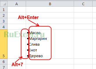
Чтобы проставить вначале списка маркеры в виде жирных точек, можно воспользоваться сочетанием клавиш Alt+7.
Перенос текста в ячейке Excel или создание нового абзаца (Enter).
Одним из наиболее популярных вопросов среди пользователей программы «Эксель» является вопрос о том, каким образом перенести текст внутри ячейки на новую строку нажатием клавиши ENTER, чтобы активная ячейка не менялась и не перескакивала ниже.
Так, например, если Вам нужно написать текст в форме списка, чтобы каждое предложение начиналось с новой строки, многие пользователи выходят из затруднительного положения при помощи следующей хитрости:
набирают текст в программе Word или ином редакторе текстовых документов, потом копируют и вставляют уже форматированный текст в ячейку Excel.
Описанная процедура довольно трудоемкая и требует выполнения множества лишних действий: открытие программы Word, перенос текста и т.д., что значительно увеличивает затраченное время при использовании слабого компьютера.
Существует гораздо более быстрый и простой способ переноса текста в новую строку в ячейках Excel.
Для переноса текста достаточно нажать сочетание клавиш Alt + Enter, после указанного действия курсор переместится на строчку ниже, не перескакивая на новую ячейку, и Вы сможете набирать текст с новой строки. Похожая хитрость есть и для других офисных программ Libro или Open Office, только следует использовать сочетание Ctrl + Enter.
Чтобы проставить вначале списка маркеры в виде жирных точек, можно воспользоваться сочетанием клавиш Alt+7.
Как сделать перенос текста в ячейке в Excel
Если Вы периодически создаете документы в программе Microsoft Excel, тогда заметили, что все данные, которые вводятся в ячейку, прописываются в одну строчку. Поскольку это не всегда может подойти, и вариант растянуть ячейку так же не уместен, возникает необходимость переноса текста. Привычное нажатие «Enter» не подходит, поскольку курсор сразу перескакивает на новую строку, и что делать дальше?
Вот в этой статье мы с Вами и научимся переносить текст в Excel на новую строку в пределах одной ячейки. Рассмотрим, как это можно сделать различными способами.
Использовать для этого можно комбинацию клавиш «Alt+Enter» . Поставьте курсив перед тем словом, которое должно начинаться с новой строки, нажмите «Alt» , и не отпуская ее, кликните «Enter» . Все, курсив или фраза перепрыгнет на новую строку. Напечатайте таким образом весь текст, а потом нажмите «Enter» .

Выделится нижняя ячейка, а нужная нам увеличится по высоте и текст в ней будет виден полностью.
Чтобы быстрее выполнять некоторые действия, ознакомьтесь со списком горячих клавиш в Эксель.
Для того чтобы во время набора слов, курсив перескакивал автоматически на другую строку, когда текст уже не вмещается по ширине, сделайте следующее. Выделите ячейку и кликните по ней правой кнопкой мыши. В контекстном меню нажмите «Формат ячеек» .
Вверху выберите вкладку «Выравнивание» и установите птичку напротив пункта «переносить по словам» . Жмите «ОК» .
Напишите все, что нужно, а если очередное слово не будет вмещаться по ширине, оно начнется со следующей строки.
Если в документе строки должны переноситься во многих ячейках, тогда предварительно выделите их, а потом поставьте галочку в упомянутом выше окне.
В некоторых случаях, все то, о чем я рассказала выше, может не подойти, поскольку нужно, чтобы информация с нескольких ячеек была собрана в одной, и уже в ней поделена на строки. Поэтому давайте разбираться, какие формулы использовать, чтобы получить желаемый результат.
Одна из них – это СИМВОЛ() . Здесь в скобках нужно указать значение от единицы до 255. Число берется со специальной таблицы, в которой указано, какому символу оно соответствует. Для переноса строчки используется код 10.
Теперь о том, как работать с формулой. Например, возьмем данные с ячеек A1:D2 и то, что написано в разных столбцах ( A, B, C, D ), сделаем в отдельных строчках.
Ставлю курсив в новую ячейку и в строку формул пишу:
Знаком «&» мы сцепляем ячейки А1:А2 и так далее. Нажмите «Enter» .
Не пугайтесь результата – все будет написано в одну строку. Чтобы это поправить, откройте окно «Формат ячеек» и поставьте галочку в пункте перенос, про это написано выше.
В результате, мы получим то, что хотели. Информация будет взята с указанных ячеек, а там, где было поставлено в формуле СИМВОЛ(10) , сделается перенос.
Для переноса текста в ячейке используется еще одна формула – СЦЕПИТЬ() . Давайте возьмем только первую строку с заголовками: Фамилия, Долг, К оплате, Сумма. Кликните по пустой ячейке и введите формулу:
Вместо A1, B1, C1, D1 укажите нужные Вам. Причем их количество можно уменьшить или увеличить.
Результат у нас получится такой.
Поэтому открываем уже знакомое окно Формата ячеек и отмечаем пункт переноса. Теперь нужные слова будут начинаться с новых строчек.
В соседнюю ячейку я вписала такую же формулу, только указала другие ячейки: A2:D2 .
Плюс использования такого метода, как и предыдущего, в том, что при смене данных в исходных ячейках, будут меняться значения и в этих.
В примере изменилось число долга. Если еще и посчитать автоматически сумму в Экселе, тогда менять вручную больше ничего не придется.
Если же у Вас уже есть документ, в котором много написано в одной ячейке, и нужно слова перенести, тогда воспользуемся формулой ПОДСТАВИТЬ() .
Суть ее в том, что мы заменим все пробелы на символ переноса строчки. Выберите пустую ячейку и добавьте в нее формулу:
Вместо А11 будет Ваш исходный текст. Нажмите кнопку «Enter» и сразу каждое слово отобразится с новой строки.
Кстати, чтобы постоянно не открывать окно Формат ячеек, можно воспользоваться специальной кнопкой «Перенести текст» , которая находится на вкладке «Главная» .
Думаю, описанных способов хватит, чтобы перенести курсив на новую строку в ячейке Excel. Выбирайте тот, который подходит больше всего для решения поставленной задачи.
Как в Excel сделать перенос текста в ячейке
Часто требуется внутри одной ячейки Excel сделать перенос текста на новую строку. То есть переместить текст по строкам внутри одной ячейки как указано на картинке. Если после ввода первой части текста просто нажать на клавишу ENTER, то курсор будет перенесен на следующую строку, но другую ячейку, а нам требуется перенос в этой же ячейке.
Это очень частая задача и решается она очень просто — для переноса текста на новую строку внутри одной ячейки Excel необходимо нажать ALT+ENTER (зажимаете клавишу ALT, затем не отпуская ее, нажимаете клавишу ENTER)
Как перенести текст на новую строку в Excel с помощью формулы
Иногда требуется сделать перенос строки не разово, а с помощью функций в Excel. Вот как в этом примере на рисунке. Мы вводим имя, фамилию и отчество и оно автоматически собирается в ячейке A6
Для начала нам необходимо сцепить текст в ячейках A1 и B1 ( A1&B1 ), A2 и B2 ( A2&B2 ), A3 и B3 ( A3&B3 )
После этого объединим все эти пары, но так же нам необходимо между этими парами поставить символ (код) переноса строки. Есть специальная таблица знаков (таблица есть в конце данной статьи), которые можно вывести в Excel с помощью специальной функции СИМВОЛ(число), где число это число от 1 до 255, определяющее определенный знак.
Например, если прописать =СИМВОЛ(169), то мы получим знак копирайта ©
Нам же требуется знак переноса строки, он соответствует порядковому номеру 10 — это надо запомнить.
Код (символ) переноса строки — 10
Следовательно перенос строки в Excel в виде функции будет выглядеть вот так СИМВОЛ(10)
Примечание: В VBA Excel перенос строки вводится с помощью функции Chr и выглядит как Chr (10)
Итак, в ячейке A6 пропишем формулу
= A1&B1 &СИМВОЛ(10)& A2&B2 &СИМВОЛ(10)& A3&B3
В итоге мы должны получить нужный нам результат.
Обратите внимание! Чтобы перенос строки корректно отображался необходимо включить «перенос по строкам» в свойствах ячейки.
Для этого выделите нужную нам ячейку (ячейки), нажмите на правую кнопку мыши и выберите «Формат ячеек. »
В открывшемся окне во вкладке «Выравнивание» необходимо поставить галочку напротив «Переносить по словам» как указано на картинке, иначе перенос строк в Excel не будет корректно отображаться с помощью формул.
Как в Excel заменить знак переноса на другой символ и обратно с помощью формулы
Можно поменять символ перенос на любой другой знак, например на пробел, с помощью текстовой функции ПОДСТАВИТЬ в Excel
Рассмотрим на примере, что на картинке выше. Итак, в ячейке B1 прописываем функцию ПОДСТАВИТЬ:
A1 — это наш текст с переносом строки;
СИМВОЛ(10) — это перенос строки (мы рассматривали это чуть выше в данной статье);
» » — это пробел, так как мы меняем перенос строки на пробел
Если нужно проделать обратную операцию — поменять пробел на знак (символ) переноса, то функция будет выглядеть соответственно:
Напоминаю, чтобы перенос строк правильно отражался, необходимо в свойствах ячеек, в разделе «Выравнивание» указать «Переносить по строкам».
Как поменять знак переноса на пробел и обратно в Excel с помощью ПОИСК — ЗАМЕНА
Бывают случаи, когда формулы использовать неудобно и требуется сделать замену быстро. Для этого воспользуемся Поиском и Заменой. Выделяем наш текст и нажимаем CTRL+H, появится следующее окно.
Если нам необходимо поменять перенос строки на пробел, то в строке «Найти» необходимо ввести перенос строки, для этого встаньте в поле «Найти», затем нажмите на клавишу ALT , не отпуская ее наберите на клавиатуре 010 — это код переноса строки, он не будет виден в данном поле.
После этого в поле «Заменить на» введите пробел или любой другой символ на который вам необходимо поменять и нажмите «Заменить» или «Заменить все».
Кстати, в Word это реализовано более наглядно.
Если вам необходимо поменять символ переноса строки на пробел, то в поле «Найти» вам необходимо указать специальный код «Разрыва строки», который обозначается как ^l
В поле «Заменить на: » необходимо сделать просто пробел и нажать на «Заменить» или «Заменить все».
Вы можете менять не только перенос строки, но и другие специальные символы, чтобы получить их соответствующий код, необходимо нажать на кнопку «Больше >> «, «Специальные» и выбрать необходимый вам код. Напоминаю, что данная функция есть только в Word, в Excel эти символы не будут работать.
Как поменять перенос строки на пробел или наоборот в Excel с помощью VBA
Рассмотрим пример для выделенных ячеек. То есть мы выделяем требуемые ячейки и запускаем макрос
1. Меняем пробелы на переносы в выделенных ячейках с помощью VBA
Sub ПробелыНаПереносы()
For Each cell In Selection
cell.Value = Replace (cell.Value, Chr (32) , Chr (10) )
Next
End Sub
2. Меняем переносы на пробелы в выделенных ячейках с помощью VBA
Sub ПереносыНаПробелы()
For Each cell In Selection
cell.Value = Replace (cell.Value, Chr (10) , Chr (32) )
Next
End Sub
Код очень простой Chr (10) — это перенос строки, Chr (32) — это пробел. Если требуется поменять на любой другой символ, то заменяете просто номер кода, соответствующий требуемому символу.
Коды символов для Excel
Ниже на картинке обозначены различные символы и соответствующие им коды, несколько столбцов — это различный шрифт. Для увеличения изображения, кликните по картинке.
Перенос текста в ячейке
Microsoft Excel обеспечивает перенос текста в ячейке для его отображения на нескольких строках. Ячейку можно настроить для автоматического переноса текста или ввести разрыв строки вручную.
Автоматический перенос текста
Выделите на листе ячейки, которые требуется отформатировать.
На вкладке Главная в группе Выравнивание выберите команду Перенести текст  .
.
Данные в ячейке будут переноситься в соответствии с шириной столбца, поэтому при ее изменении перенос текста будет настраиваться автоматически.
Если текст с переносами отображается не полностью, возможно, задана точная высота строки или текст находится в объединенных ячейках.
Настройка высоты строки для отображения всего текста
Выделите ячейки, для которых требуется выровнять высоту строк.
На вкладке Главная в группе Ячейки нажмите кнопку Формат.
В группе Размер ячейки выполните одно из следующих действий:
Чтобы автоматически выравнивать высоту строк, выберите команду Автоподбор высоты строки.
Чтобы задать высоту строк, выберите команду Высота строки и введите нужное значение в поле Высота строки.
Совет: Кроме того, можно перетащить нижнюю границу строки в соответствии с высотой текста в строке.
Ввод разрыва строки
Новую строку текста можно начать в любом месте ячейки.
Дважды щелкните ячейку, в которую требуется ввести разрыв строки.
Совет: Можно также выделить ячейку, а затем нажать клавишу F2.
Дважды щелкните в ячейке то место, куда нужно вставить разрыв строки, и нажмите сочетание клавиш ALT+ВВОД.
Дополнительные сведения
Вы всегда можете задать вопрос специалисту Excel Tech Community, попросить помощи в сообществе Answers community, а также предложить новую функцию или улучшение на веб-сайте Excel User Voice.
Перенос строки в пределах ячейки в Microsoft Excel
Как известно, по умолчанию в одной ячейке листа Excel располагается одна строка с числами, текстом или другими данными. Но, что делать, если нужно перенести текст в пределах одной ячейки на другую строку? Данную задачу можно выполнить, воспользовавшись некоторыми возможностями программы. Давайте разберемся, как сделать перевод строки в ячейке в Excel.
Способы переноса текста
Некоторые пользователи пытаются перенести текст внутри ячейки нажатием на клавиатуре кнопки Enter. Но этим они добиваются только того, что курсор перемещается на следующую строку листа. Мы же рассмотрим варианты переноса именно внутри ячейки, как очень простые, так и более сложные.
Способ 1: использование клавиатуры
Самый простой вариант переноса на другую строку, это установить курсор перед тем отрезком, который нужно перенести, а затем набрать на клавиатуре сочетание клавиш Alt+Enter.
В отличие от использования только одной кнопки Enter, с помощью этого способа будет достигнут именно такой результат, который ставится.
Способ 2: форматирование
Если перед пользователем не ставится задачи перенести на новую строку строго определенные слова, а нужно только уместить их в пределах одной ячейки, не выходя за её границы, то можно воспользоваться инструментом форматирования.
-
Выделяем ячейку, в которой текст выходит за пределы границ. Кликаем по ней правой кнопкой мыши. В открывшемся списке выбираем пункт «Формат ячеек…».
После этого, если данные будут выступать за границы ячейки, то она автоматически расширится в высоту, а слова станут переноситься. Иногда приходится расширять границы вручную.
Чтобы подобным образом не форматировать каждый отдельный элемент, можно сразу выделить целую область. Недостаток данного варианта заключается в том, что перенос выполняется только в том случае, если слова не будут вмещаться в границы, к тому же разбитие осуществляется автоматически без учета желания пользователя.
Способ 3: использование формулы
Также можно осуществить перенос внутри ячейки при помощи формул. Этот вариант особенно актуален в том случае, если содержимое выводится с помощью функций, но его можно применять и в обычных случаях.
- Отформатируйте ячейку, как указано в предыдущем варианте.
- Выделите ячейку и введите в неё или в строку формул следующее выражение:
Вместо элементов «ТЕКСТ1» и «ТЕКСТ2» нужно подставить слова или наборы слов, которые хотите перенести. Остальные символы формулы изменять не нужно.
Главным недостатком данного способа является тот факт, что он сложнее в выполнении, чем предыдущие варианты.
В целом пользователь должен сам решить, каким из предложенных способов оптимальнее воспользоваться в конкретном случае. Если вы хотите только, чтобы все символы вмещались в границы ячейки, то просто отформатируйте её нужным образом, а лучше всего отформатировать весь диапазон. Если вы хотите устроить перенос конкретных слов, то наберите соответствующее сочетание клавиш, как рассказано в описании первого способа. Третий вариант рекомендуется использовать только тогда, когда данные подтягиваются из других диапазонов с помощью формулы. В остальных случаях использование данного способа является нерациональным, так как имеются гораздо более простые варианты решения поставленной задачи.
Отблагодарите автора, поделитесь статьей в социальных сетях.