Enter in excel cell formula - Word и Excel - помощь в работе с программами

The summation formula is the simplest arithmetic operation. But any task becomes more complicated if you need to quickly perform a large amount of work.

Let`s consider on specific examples, how and what formula to enter in Excel when summing, using different input methods.

How to enter formulas in Excel cells?

In the cells A1, A1 and A3 you need to insert the numbers 1, 2 and 3, respectively. In the A4, sum ones.

How to enter formulas manually?

First, consider the manual input method:

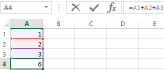
In the cell A4 enter the following formula: = A1 + A2 + A3 and press the «Enter» key.

As you can see in the picture, the cell displays the value of the amout, and the formula itself can be seen in the formula bar. For a detailed analysis of the cell references, you can switch to a special sheet view mode with the CTRL + `key combination. Pressing this combination again switches to normal operation.

Note that the addresses of the cells are highlighted in different colors.

The same colors are used to frame the cells to that the address refers. This simplifies to the visual analysis during operation.

Attention. The computational function of the formulas is dynamic. For example, if we change the value of the cell A1 to 3, then the amount will automatically change to 8.

The notation. In the Excel settings, you can disable the automatic recalculation of values. In manual mode, the values are recalculated after pressing the F9 key, but most often the working in this mode is not necessary.

How to enter formulas using the mouse?

Consider now how to enter a formula in Excel correctly. Entering links can be performed much faster using the mouse:

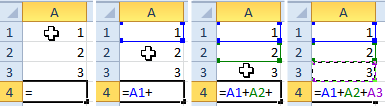
Go to the cell A4 and paste the symbol «=». Thus, you specify that the next value is a formula or a function.
Click on the cell A1 and enter the «+» sign.
Click on the cell A2 and press the «+» key again.
Last click on A3 and press Enter to enter the formula and get the result of the calculation when summing the values.

How to enter formulas using the keyboard?

You can also enter cell addresses into formulas using the keyboard arrow keys (arrows).

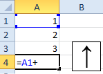
Since any formula starts with an equal sign, in the A4 insert «=».
Press 3 times on the keypad «up arrow» and the cursor will move to the cell A1. And its address will be automatically entered in A4. Then you need to click «+».
Accordingly, press «up arrow» 2 times and get the reference to A2. Then we press «+».
Now we press only the «up arrow» key once, and then Enter for input of the data in the cell.

Managing the links in the formulas with the arrow keys of the keyboard slightly resembles the previous method.

Similarly, you can insert the links to entire ranges, just after the «=» sign you need to select the required range of cells. You already know how to select ones using the mouse or the «arrows» of the keyboard from previous lessons.

Источник

Create a simple formula in Excel

Excel for Microsoft 365 Excel for Microsoft 365 for Mac Excel 2021 Excel 2021 for Mac Excel 2019 Excel 2019 for Mac Excel 2016 Excel 2016 for Mac Excel 2013 Excel 2010 Excel 2007 Excel for Mac 2011 More…Less

You can create a simple formula to add, subtract, multiply or divide values in your worksheet. Simple formulas always start with an equal sign (=), followed by constants that are numeric values and calculation operators such as plus (+), minus (—), asterisk(*), or forward slash (/) signs.

Let’s take an example of a simple formula.

On the worksheet, click the cell in which you want to enter the formula.
Type the = (equal sign) followed by the constants and operators (up to 8192 characters) that you want to use in the calculation.

For our example, type =1+1.
Notes:
- Instead of typing the constants into your formula, you can select the cells that contain the values that you want to use and enter the operators in between selecting cells.
- Following the standard order of mathematical operations, multiplication and division is performed before addition and subtraction.
Press Enter (Windows) or Return (Mac).

Let’s take another variation of a simple formula. Type =5+2*3 in another cell and press Enter or Return. Excel multiplies the last two numbers and adds the first number to the result.

Use AutoSum

You can use AutoSum to quickly sum a column or row or numbers. Select a cell next to the numbers you want to sum, click AutoSum on the Home tab, press Enter (Windows) or Return (Mac), and that’s it!

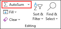
When you click AutoSum, Excel automatically enters a formula (that uses the SUM function) to sum the numbers.

Note: You can also type ALT+= (Windows) or ALT++= (Mac) into a cell, and Excel automatically inserts the SUM function.

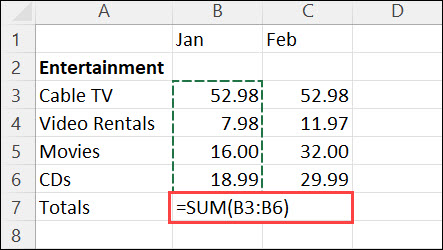
Here’s an example. To add the January numbers in this Entertainment budget, select cell B7, the cell immediately below the column of numbers. Then click AutoSum. A formula appears in cell B7, and Excel highlights the cells you’re totaling.

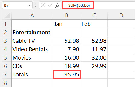
Press Enter to display the result (95.94) in cell B7. You can also see the formula in the formula bar at the top of the Excel window.

Notes:

To sum a column of numbers, select the cell immediately below the last number in the column. To sum a row of numbers, select the cell immediately to the right.
Once you create a formula, you can copy it to other cells instead of typing it over and over. For example, if you copy the formula in cell B7 to cell C7, the formula in C7 automatically adjusts to the new location, and calculates the numbers in C3:C6.
You can also use AutoSum on more than one cell at a time. For example, you could highlight both cell B7 and C7, click AutoSum, and total both columns at the same time.

Copy the example data in the following table, and paste it in cell A1 of a new Excel worksheet. If you need to, you can adjust the column widths to see all the data.

Note: For formulas to show results, select them, press F2, and then press Enter (Windows) or Return (Mac).

Data
2
5
Formula	Description	Result
=A2+A3	Adds the values in cells A1 and A2	=A2+A3
=A2-A3	Subtracts the value in cell A2 from the value in A1	=A2-A3
=A2/A3	Divides the value in cell A1 by the value in A2	=A2/A3
=A2*A3	Multiplies the value in cell A1 times the value in A2	=A2*A3
=A2^A3	Raises the value in cell A1 to the exponential value specified in A2	=A2^A3
Formula	Description	Result
=5+2	Adds 5 and 2	=5+2
=5-2	Subtracts 2 from 5	=5-2
=5/2	Divides 5 by 2	=5/2
=5*2	Multiplies 5 times 2	=5*2
=5^2	Raises 5 to the 2nd power	=5^2

Need more help?

You can always ask an expert in the Excel Tech Community or get support in the Answers community.

Need more help?

Want more options?

Explore subscription benefits, browse training courses, learn how to secure your device, and more.

Communities help you ask and answer questions, give feedback, and hear from experts with rich knowledge.

Источник

Download Article

Microsoft Excel’s power is in its ability to calculate and display results from data entered into its cells. To calculate anything in Excel, you need to enter formulas into its cells. Formulas can be simple arithmetical formulas or complicated formulas involving conditional statements and nested functions. All Excel formulas use a basic syntax, which is described in the steps below.

1

Begin every formula with an equal sign (=). The equal sign tells Excel that the string of characters you’re entering into a cell is a mathematical formula. If you forget the equal sign, Excel will treat the entry as a character string.
2
Use coordinate references for cells that contain the values used in your formula. While you can include numeric constants in your formulas, in most cases you’ll use values entered in other cells (or the results of other formulas displayed in those cells) in your formulas. You refer to those cells with a coordinate reference of the row and column the cell is in. There are several formats:
- The most common coordinate reference is to use the letter or letters representing the column followed by the number of the row the cell is in: A1 refers to the cell in Column A, Row 1. If you add rows above the referenced cell or columns above the referenced cell, the cell’s reference will change to reflect its new position; adding a row above Cell A1 and a column to its left will change its reference to B2 in any formula the cell is referenced in.
- A variation of this reference is to make row or column references absolute by preceding them with a dollar sign ($). While the reference name for Cell A1 will change if a row is added above or a column is added in front of it, Cell $A$1 will always refer to the cell in the upper left corner of the spreadsheet; thus, in a formula, Cell $A$1, could have a different, or even invalid, value in the formula if rows or columns are inserted in the spreadsheet. (You can make only the row or column cell reference absolute, if you wish.)
- Another way to reference cells is numerically, in the format RxCy, where «R» indicates «row,» «C» indicates «column,» and «x» and «y» are the row and column numbers. Cell R5C4 in this format would be the same as Cell $D$5 in absolute column, row reference format. Putting either number after the «R» or the «C» makes that reference relative to the upper left corner of the spreadsheet page.
- If you use only an equal sign and a single cell reference in your formula, you copy the value from the other cell into your new cell. Entering the formula «=A2» in Cell B3 will copy the value entered into Cell A2 into Cell B3. To copy the value from a cell in one spreadsheet page to a cell on a different page, include the page name, followed by an exclamation point (!). Entering «=Sheet1!B6» in Cell F7 on Sheet2 of the spreadsheet displays the value of Cell B6 on Sheet1 in Cell F7 on Sheet2.
Advertisement
3
Use arithmetic operators for basic calculations. Microsoft Excel can perform all of the basic arithmetic operations �- addition, subtraction, multiplication, and division -� as well as exponentiation. Some operations use different symbols than are used when writing equations by hand. A list of operators is given below, in the order in which Excel processes arithmetic operations:
- Negation: A minus sign (-). This operation returns the additive inverse of the number represented by the numeric constant or cell reference following the minus sign. (The additive inverse is the value added to a number to produce a value of zero; it’s the same as multiplying the number by -1.)
- Percentage: The percent sign (%). This operation returns the decimal equivalent of the percentage of the numeric constant in front of the number.
- Exponentiation: A caret (^). This operation raises the number represented by the cell reference or constant in front of the caret to the power of the number after the caret.
- Multiplication: An asterisk (*). An asterisk is used for multiplication to avoid confusion with the letter «x.»
- Division: A forward slash (/). Multiplication and division have equal precedence and are performed from left to right.
- Addition: A plus sign (+).
- Subtraction: A minus sign (-). Addition and subtraction have equal precedence and are performed from left to right.
4
Use comparison operators to compare the values in cells. You’ll use comparison operators most often in formulas with the IF function. You place a cell reference, numeric constant, or function that returns a numeric value on either side of the comparison operator. The comparison operators are listed below:
- Equals: An equal sign (=).
- Is not equal to (<>).
- Less than (<).
- Less than or equal to (<=).
- Greater than (>).
- Greater than or equal to (>=).
5

Use an ampersand (&) to join text strings together. The joining of text strings into a single string is called concatenation, and the ampersand is known as a text operator when used to join strings together in Excel formulas. You can use it with text strings or cell references or both; entering «=A1&B2» in Cell C3 will yield «BATMAN» when «BAT» is entered in Cell A1 and «MAN» is entered in Cell B2.
6
Use reference operators when working with ranges of cells. You’ll use ranges of cells most often with Excel functions such as SUM, which finds the sum of a range of cells. Excel uses 3 reference operators:
- Range operator: a colon (:). The range operator refers to all cells in a range beginning with the referenced cell in front of the colon and ending with the referenced cell after the colon. All the cells are usually in the same row or column; «=SUM(B6:B12)» displays the result of adding the column of cells from B6 through B12, while «=AVERAGE(B6:F6)» displays the average of the numbers in the row of cells from B6 through F6.
- Union operator: a comma (,). The union operator includes both the cells or ranges of cells named before the comma and those after it; «=SUM(B6:B12, C6:C12)» adds together the cells from B6 through B12 and C6 through C12.
- Intersection operator: a space ( ). The intersection operator identifies cells common to 2 or more ranges; listing the cell ranges «=B5:D5 C4:C6» yields the value in the cell C5, which is common to both ranges.
7
Use parentheses to identify the arguments of functions and to override the order of operations. Parentheses serve 2 functions in Excel, to identify the arguments of functions and to specify a different order of operations than the normal order.
- Functions are pre-defined formulas. Some, such as SIN, COS, or TAN, take a single argument, while other functions, such as IF, SUM, or AVERAGE, may take multiple arguments. Multiple arguments within a function are separated by commas, as in «=IF (A4 >=0, «POSITIVE,» «NEGATIVE»)» for the IF function. Functions may be nested within other functions, up to 64 levels deep.
- In mathematical operation formulas, operations within parentheses are performed before those outside it; in «=A4+B4*C4,» B4 is multiplied by C4 before A4 is added to the result, but in «=(A4+B4)*C4,» A4 and B4 are added together first, then the result is multiplied by C4. Parentheses in operations may be nested inside each other; the operation in the innermost set of parentheses will be performed first.
- Whether nesting parentheses in mathematical operations or in nested functions, always be sure to have as many close parentheses in your formula as you do open parentheses, or you’ll receive an error message.

1

Select the cell you want to enter the formula in.
2

Type an equal sign the cell or in the formula bar. The formula bar is located above the rows and columns of cells and beneath the menu bar or ribbon.
3

Type an open parenthesis if necessary. Depending on the structure of your formula, you may need to type several open parentheses.
4

Create a cell reference. You can do this in 1 of several ways: Type the cell reference manually.Select a cell or range of cells in the current page of the spreadsheet.Select a cell or range of cells in another page of the spreadsheet.Select a cell or range of cells on a page of a different spreadsheet.
5

Enter a mathematical, comparison, text, or reference operator if desired. For most formulas, you’ll use a mathematical operator or 1 of the reference operators.
6

Repeat the previous 3 steps as necessary to build your formula.
7

Type a close parenthesis for each open parenthesis in your formula.
8

Press «Enter» when your formula is the way you want it to be.

Add New Question

Question

What is the name of «;»?

It is called a semicolon, which can be used in programming languages to separate the statements or print variables by using one output statement.
Question

How do I subtract one cell from another in Excel?

If you want to subtract cell A1 from cell B1, in cell C1 you would type «=A1-B1» and hit enter. You can also use the autosum feature in the far right of the header.
Question

How do I type the symbols that are used in Excel?

You click Shift and the number/letter you see the symbol on (for example, if you want the multiplication symbol * you hit Shift+8) when using a keyboard. On a phone you have to switch the keyboard to the special characters one and find the symbol you want.

See more answers

Ask a Question

200 characters left

Include your email address to get a message when this question is answered.

Submit

When you first start working with complex formulas, it may be helpful to write the formula out on paper before entering it into Excel. If the formula looks too complex to enter into a single cell, you can break it down into several parts and enter the parts into several cells, and use a simpler formula in another cell to combine the results of the individual formula parts together.
Microsoft Excel offers assistance in typing formulas with Formula AutoComplete, a dynamic list of functions, arguments, or other possibilities that appears after you type the equal sign and the first few characters of your formula. Press your «Tab» key or double-click an item in the dynamic list to insert it in your formula; if the item is a function, you will then be prompted to enter its arguments. You can turn this feature on or off by selecting «Formulas» on the «Excel Options» dialog and checking or unchecking the «Formula AutoComplete» box. (You access this dialog by selecting «Options» from the «Tools» menu in Excel 2003, from the «Excel Options» button on the «File» button menu in Excel 2007, and by selecting «Options» on the «File» tab menu in Excel 2010.)
When renaming the sheets in a multi-page spreadsheet, make it a practice not to use any spaces in the new sheet name. Excel won’t recognize naked spaces in sheet names in formula references. (You can also get around this problem by substituting an underscore for the space in the sheet name when using it in a formula.)

Thanks for submitting a tip for review!

Don’t include formatting such as commas or dollar signs in numbers when entering them in formulas because Excel recognizes commas as argument separators and union operators and dollar signs as absolute reference indicators.

About This Article

Thanks to all authors for creating a page that has been read 302,610 times.

Is this article up to date?

Источник

Write Basic Formulas in Excel

Formulas are an integral part of Excel. As a new learner of Excel, one does not understand the importance of formulas in Excel. However, all the new learners know plenty of built-in formulas but do not know how to apply them.

In this article, we will show you how to write formulas in Excel and dynamically change them when the referenced cell values are changed automatically.

Write Basic Formulas in Excel
- How to Write/Insert Formulas in Excel?
  - Example #1
  - Example #2
- How to use Built-in Excel Functions?
  - Example #1 – SUM Function
  - Example #2 – AVERAGE Function
- Things to Remember about Inserting Formula in Excel
- Recommended Articles

How to Write/Insert Formulas in Excel?

You can download this Write Formula Excel Template here – Write Formula Excel Template

To write a formula in Excel, you first need to enter the equal sign in the cell where we need to enter the formula. So, the formula always starts with an equal (=) sign.

Example #1

Look at the below data in the Excel worksheet.

We have two numbers in A1 and A2 cells, respectively. So, if we want to add these two numbers in cell A3, we must first open the equal sign in the A3 cell.

Enter the numbers as 525 + 800.

Press the “Enter” key to get the formula equation’s result.

The formula bar shows the formula, not the result of the formula.

As you can see above, we have got the result as 1325 as the summation of the numbers 525 and 800. In the formula bar, we can see how the formula has been applied = 525+800.

Now, we will change the A1 and A2 numbers to 50 and 80, respectively.

Result cell A3 shows the old formula result only. It is where we need to make dynamic cell referenceCell reference in excel is referring the other cells to a cell to use its values or properties. For instance, if we have data in cell A2 and want to use that in cell A1, use =A2 in cell A1, and this will copy the A2 value in A1.read more formulas.

Instead of entering the two cell numbers, give a cell reference only to the formula.

Press the “Enter” key to get the result of this formula.

In the formula bar, we can see the formula as A1 + A2, not the numbers of the A1 and A2 cells. Now, change the numbers of any of the cells. For example, in the A3 cell, it will automatically impact the result.

We have changed the A1 cell number from 50 to 100, and because the A3 cell has the reference of the cells A1 and A2, the A3 cell automatically changed.

Example #2

Now, we have other numbers for the adjacent columns.

We have numbers in four more columns. We need to get the total of these numbers as we did for A1 and A3 cells.

It is where the real power of cell-references formulas is crucial in making the formula dynamic. For example, copy cell A3, which has already applied the formula A1 + A2, and paste it to the next cell, B3.

Look at the result in cell B3. The formula bar says the formula as B1 + B2 instead of A1 + A2.

When we copied and pasted the A3 cell, the formula cell, we moved one column to the right. But in the same row, we have passed the formula. Because we moved one column to the right in the same row-column reference or header value, “A” has been changed to “B,” but row numbers 1 and 2 remain the same.

Copy and paste the formula to other cells to get the total in all the cells.

How to use Built-in Excel Functions?

Example #1 – SUM Function

We have plenty of built-in functions in Excel according to the requirements and situations we can use. For example, look at the below data in Excel.

We have numbers from the A1 to E5 range of cells. In the B7 cell, we need the total sum of these numbers. Adding individual cell references and entering each cell reference one by one consumes a lot of time, so putting an equal sign open SUM function in excelThe SUM function in excel adds the numerical values in a range of cells. Being categorized under the Math and Trigonometry function, it is entered by typing “=SUM” followed by the values to be summed. The values supplied to the function can be numbers, cell references or ranges.read more.

Select the range of cells from A1 to E5 and close the bracket.

Press the “Enter” key to get the total numbers from A1 to E5.

In just a fraction of seconds, we got the total numbers. In the formula bar, we can see the formula as =SUM(A1: E5).

Example #2 – AVERAGE Function

Assume you have students” every subject score, and you need to find the student’s average score. It is possible to find an average score in a fraction of seconds. For example, look at the below data.

Open AVERAGE function in the H2 cell first.

Select the range of cells reference as B2 to G2 because for the student “Amit,” all the subject scores are in this range only.

Press the “Enter” key to get the average student “Amit.”

So, the student “Amit” average score is 79.

Now, drag formula cell H2 to the below cells to get the average of other students.

Things to Remember about Inserting Formula in Excel

The formula should always start with an equal sign. We can also start with a PLUS or MINUS sign but not recommended.
While doing calculations, we need to remember BODMAS’s basic Maths rules.
We must always use built-in functions in Excel.

How to enter a formula in Excel

In Excel, each cell can contain a calculation. In Excel jargon we call this a formula. Each cell can contain one formula. When you enter a formula in a cell, Excel calculates the result of that formula and displays the result of that calculation to you. In fact, when you enter a formula into any cell, Excel will recalculate the result of all the cells in the worksheet. This normally happens in the blink of an eye so you won’t normally notice it, although you may find that large and complex spreadsheets can take longer to recalculate.

When entering a formula, you have to make sure Excel knows that’s what you want to do. You start by typing the = (equals) sign, then the rest of your formula. If you don’t type the equals sign first, then Excel will assume you are typing either a number or a text. You can also start a formula with either a plus (+) or minus (-) symbol. Excel will assume you’re typing a formula and insert the equals sign for you.

Here are some examples of some simple Excel formulas and their results:

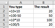
In this example, there are four basic formulas:

Addition (+)
Subtraction (—)
Multiplication (*)
Division (/)

In each case, you would type the equals sign (=), then the formula, then press Enter to tell Excel you’ve finished.

Sometimes Excel will show you a warning rather than just entering your formula. This will happen if the formula you’ve typed is invalid, i.e. is not in a format that Excel recognises. It will usually also give you some indication of what you did wrong.
Other times, Excel may enter the formula you have typed correctly but then show you an error such as #VALUE. This means that you have entered a formula that was value, but Excel could not calculate a valid result from your formula.

Creating formulas that refer to other cells in the same worksheet

Excel’s power comes from allowing you to create formulas that refer to the values in other cells.

In the example above, you’ll notice the headings across the top (A, B) and down the left (1,2,3,4,5). By comining these values, we have a unique reference each cell in a worksheet (A1, A2, A3, B1, B2, B3, and so on).

When you create a formula, you can refer to other cells using these cell references to incorporate the values in other cells into a formula. The value in another cell might be a simple number, or another cell containing a formula. When you create a formula that refers to another cell that also contains a formula, your formula will use the result of the formula in that other cell. Then, if the result of the formula in that other cell changes, so too does the result in your formula.

Here are some examples of some Excel formulas that refer to other cells:

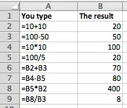
In this example, rows 6-8 build on the earlier examples to link cells together:

B6 adds the values in B2 and B3 together. If you change either of the values in B2 or B3 the result in B6 will change too.
B7 and B8 subtract and multiply the values in other cells.
B9 goes a step further and divides B8 by B3. Note that B8 in turn multiplied B5 and B2 together. So changing the values in either B5 or B2 will have a domino effect, where the value in B8 will change, and so the value in B9 will change too. Note that Excel handles all of this the moment you finish entering a change in either B5 or B2.

Creating formulas that refer to cells in other worksheets

When you first open Excel, you start with a single worksheet. However, Excel allows you to have more than one worksheet inside a single spreadsheet file (known as a workbook). In fact, in earlier versions of Excel a new workbook automatically started out with 3 worksheets inside it.

Earlier we saw how to link two cells together within a worksheet by referring to other cells using their cell reference value. Referring to a cell inside another worksheet works in much the same way, but we need to provide more information about the location of that cell so Excel knows which cell we’re talking about.

Here are some examples of formulas that refer to cells in another worksheet inside the same workbook:

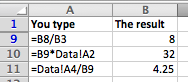
In this example, the formulas in B10 and B11 refer to cells in another worksheet called Data.

B10 multiples the value in B9 by the value in cell A2 in the worksheet called Data
B11 takes the value A4 in the worksheet called Data and divides it by the value in B9.

In other words, we’ve told Excel to go to the worksheet called Data and use values in that worksheet in our formulas.

There are a couple of ways to create formulas like this:

Type the formula in by hand. In the above example, you would create the reference to the other worksheet by typing the worksheet name followed by an exclamation mark (!); the exclamation mark tells Excel that you’re referring to another worksheet.
Start typing the formula by typing the equals sign (=), then click on the name of the other worksheet. Excel will switch to the other worksheet, and you can click on the cell you want to reference in your formula. You can then press Enter to finish entering the formula, or you can click back on the original worksheet name and finish typing your formula before pressing Enter.

Note that if you rename the worksheet called Data, the formulas that refer to Data will automatically update to reflect the new name. Here’s what the above examples look like if we change the name of the worksheet called Data to Daily Data.

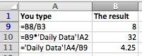
Note how Excel has put apostrophes around the name of the worksheet called Daily Data. This is because of the space in the worksheet name. Excel does this to make sure that the reference still works; if you manually type the formula without the apostrophes then Excel will not be able to validate the formula, and will not let you enter it.

Creating formulas that link to other workbooks

As you might imagine what we’ve already covered, it is also possible to create a formulat that refers to cells in another workbook (i.e. another file). Once again, it’s simply a matter of correctly referring to the cell in the other workbook.

The following example shows what this looks like:

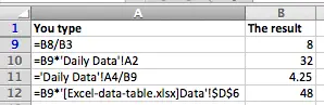
In this example, B12 contains a formula that refers to cell D6 in a worksheet called Data in a file called Excel-data-table-xlsx.

The square brackets are used to indicate the filename, i.e. [filename]. Be aware that if the file referred to is not currently open, the square brackets may also include the full file path to that file, so that Excel can still read the value from the cell being referred to even though the file is not open.
The apostrophes are used to enclose the full file name and worksheet name.
Then, Excel uses absolute references to identify the cell being referred to. This means that if you move (not copy) the contents of cell D6 in the Data worksheet, your formula will still work. The $ signs are used to denote an absolute reference (as opposed to a relative reference). Absolute and relative references are out of scope for this lesson, but you can read about them in this lesson.

Summary

Learning to use Excel formulas is one of the most important things you’ll learn to do with Excel. Hopefully this lesson has set you on the right path, and you’ll be creating spreadsheets with formulas of your own in no time at all. If you have any feedback or questions on this lesson, please comment below!

Источник

I am trying to enter a formula into a cell which contains variable called var1a?
The code that I have is:

    Worksheets("EmployeeCosts").Range("B" & var1a).Formula = ""SUM(H5:H""& var1a)

But it enters into an excel worksheet with a mistake.

asked Sep 14, 2013 at 23:48

You aren’t building your formula right.

Worksheets("EmployeeCosts").Range("B" & var1a).Formula =  "=SUM(H5:H" & var1a & ")"

This does the same as the following lines do:

Dim myFormula As String
myFormula = "=SUM(H5:H"
myFormula = myFormula & var1a
myformula = myformula & ")"

which is what you are trying to do.

Also, you want to have the = at the beginning of the formala.

SeanC

15.6k5 gold badges45 silver badges65 bronze badges

answered Sep 14, 2013 at 23:53

enderlandenderland

13.7k17 gold badges100 silver badges152 bronze badges

I would do it like this:

Worksheets("EmployeeCosts").Range("B" & var1a).Formula = _
Replace("=SUM(H5:H{SOME_VAR})","{SOME_VAR}",var1a)

In case you have some more complex formula it will be handy

answered Mar 25, 2016 at 14:20

Đức Thanh NguyễnĐức Thanh Nguyễn

8,9773 gold badges21 silver badges26 bronze badges

Источник

Updated: 04/12/2021 by

Formulas are what helped make spreadsheets so popular. By creating formulas, you can perform quick calculations even if the information changes in the cells relating to the formula. For example, you could have a total cell that adds all values in a column.

The basics

All spreadsheet formulas begin with an equal sign (=) symbol.
After the equal symbol, either a cell or formula function is entered. The function tells the spreadsheet the type of formula.
If a math function is being performed, the math formula is surrounded in parentheses. Math functions or calculations can use an operator, including plus (+), minus (-), multiply (*), divide (/), greater than (>), and less than (<).
Using the colon (:) lets you get a range of cells for a formula. For example, A1:A10 is cells A1 through A10.
Formulas are created using relative cell reference by default, and if you add a dollar sign ($) in front of the column or row, it becomes an absolute cell reference.

Entering a spreadsheet formula

Below is an animated visual example of how an excel formula can be inserted into a spreadsheet. In our first formula entered into the cell «D1,» we manually enter a =sum formula to add 1+2 (in cells A1 and B2) to get the total of «3.» With the next example, we use the mouse to highlight cells A2 to D2 and then click the formula button in Excel to automatically create the formula. Next, we show how you can manually enter a formula, and then using a mouse, get the cell values (you can also highlight multiple cells to create a range). Finally, we manually enter a times ( * ) formula using the sum function to find the value of 5 * 100.

Formula examples

Note

The functions listed below may not be the same in all languages of Microsoft Excel. All these examples are done in the English version of Microsoft Excel.

Tip

The examples below are listed in alphabetical order. If you want to start with the most common formula, we suggest starting with the =SUM formula.

=

An = (equals) creates a cell equal to another. For example, if you were to enter =A1 in B1, whatever value was in A1 would automatically be placed in B1. You could also create a formula that would make one cell equal to more than one value. For example, if cell A1 had a first name and cell B1 had a last name, you could enter =A1&» «&B1, which combines A1 with B1, with a space between each value. You can also use a concatenate formula to combine cell values.

AVERAGE

=AVERAGE(X:X)

Display the average amount between cells. For example, if you wanted to get the average for cells A1 to A30, you would type =AVERAGE(A1:A30).

COUNT

=COUNT(X:X)

Count the number of cells in a range containing only numbers. For example, you could find how many cells between A1 and A15 contain a numeric value using the =COUNT(A1:A15). If only cell A1 and A5 contained numbers, the cell containing this function would display «2» as its value.

COUNTA

=COUNTA(X:X)

Count the number of cells in a range containing any text (text and numbers, not only numbers) and are not empty. For example, you could count the number of cells containing text in cells A1 through A20 using =COUNTA(A1:A20). If seven cells were empty, the formula would return the number «13» (20-7=13).

COUNTIF

=COUNTIF(X:X,"*")

Count the cells with a certain value. For example, if you have =COUNTIF(A1:A10,»TEST») in cell A11, then any cell between A1 through A10 with the word «test» is counted as one. So, if you have five cells in that range containing the word «test,» the value «5» is shown in cell A11 (10-5=5).

IF

=IF(*)

The syntax of the IF statement is =IF(CELL=»VALUE»,»PRINT OR DO THIS»,»ELSE PRINT OR DO THIS»). For example, the formula =IF(A1=»»,»BLANK»,»NOT BLANK») makes any cell besides A1 display the text «BLANK» if A1 has nothing in it. If A1 is not empty, the cells display the text «NOT BLANK». The IF statement has more complex uses, but can generally be reduced to the structure above.

Using IF can also be useful when you may want to calculate values in a cell, but only if those cells contain values. For example, you may be dividing the values between two cells. However, if there is nothing in the cells, you would get the #DIV/0! error. Using the IF statement, you can only calculate a cell if it contains a value. For example, if you only wanted to perform a divide function if A1 contains a value, type =IF(A1=»»,»»,SUM(B1/A1)), which only divides cell B1 by A1 if A1 contains a value. Otherwise, the cell is left blank.

Getting #DIV/0! in Microsoft Excel spreadsheet.

INDIRECT

=INDIRECT("A"&"2")

Returns a reference specified by a text string. In the example above, the formula would return the value contained in cell A2.

=INDIRECT("A"&RANDBETWEEN(1,10))

Returns the value of a random cell between A1 and A10 using the indirect and randbetween (explained below) functions.

=MEDIAN(A1:A7)

Find the median of the values of cells A1 through A7. For example, four is the median for 1, 2, 3, 4, 5, 6, 7.

MIN AND MAX

=MIN/MAX(X:X)

Min and Max represent the minimum or maximum value in the cells. For example, if you want to get the minimum value between cells A1 and A30, type =MIN(A1:A30), or =MAX(A1:A30) to get the maximum.

PRODUCT

=PRODUCT(X:X)

Multiplies two or more cells together. For example, =PRODUCT(A1:A30) would multiple cells from A1 to A30 together (i.e., A1 * A2 * A3, etc).

RAND

=RAND()

Generates a random number greater than zero, but less than one. For example, «0.681359187» could be a randomly generated number placed in the formula’s cell.

RANDBETWEEN

=RANDBETWEEN(1,100)

Generate a random number between two values. In the example above, the formula would create a random whole number between 1 and 100.

ROUND

=ROUND(X,Y)

Round a number to a specific number of decimal places. X is the cell containing the number to be rounded. Y is the number of decimal places to round. Below are examples.

=ROUND(A2,2)

Rounds the number in cell A2 to one decimal place. If the number is 4.7369, the example above rounds that number to 4.74. If the number is 4.7614, it rounds to 4.76.

=ROUND(A2,0)

Rounds the number in cell A2 to zero decimal places, or the nearest whole number. If the number is 4.736, the example above would round that number to 5. If the number is 4.367, it would round to 4.

SUM

=SUM(X:X)

The most commonly used function to add, subtract, multiple, or divide values in cells. Below are different examples of this function.

=SUM(A1+A2)

Add the cells A1 and A2.

=SUM(A1:A5)

Add cells A1 through A5.

=SUM(A1,A2,A5)

Adds cells A1, A2, and A5.

=SUM(A2-A1)

Subtracts cell A1 from A2.

=SUM(A1*A2)

Multiplies cells A1 and A2.

=SUM(A1/A2)

Divides cell A1 by A2.

SUMIF

=SUMIF(X:X,"*"X:X)

Perform the SUM function only if there is a specified value in the first selected cells. An example of this would be =SUMIF(A1:A6,»TEST»,B1:B6), which only adds the values B1:B6 if the word «test» was entered somewhere between A1:A6. So if you entered «test» (not case sensitive) in A1, but had numbers in B1 through B6, it would only add the value in B1 because «test» is in A1.

See our SUMIF definition for additional information.

TODAY

=TODAY()

Would print out the current date in the cell containing the formula. The value changes each time you open your spreadsheet to reflect the current date and time. If you want to enter a date that doesn’t change, press Ctrl and ; (semicolon) to enter the date.

TREND

=TREND(X:X)

Find the common value of cells. For example, if cells A1 through A6 had 2,4,6,8,10,12 and you entered formula =TREND(A1:A6) in a different cell, you would get the value of 2 because each number is going up by 2.

TRIM

=TRIM( )

The trim formula lets you remove any unnecessary spaces at the beginning or end of a value in a cell.

How to remove extra spaces in a cell in Microsoft Excel.

VLOOKUP

=VLOOKUP(X,X:X,X,X)

The lookup, hlookup, or vlookup formula lets you search and find related values for returned results. See our lookup definition for more information about this formula.

Источник

Excel formulas allow you to identify relationships between values in your spreadsheet’s cells, perform mathematical calculations with those values, and return the resulting value in the cell of your choice. Sum, subtraction, percentage, division, average, and even dates/times are among the formulas that can be performed automatically. For example, =A1+A2+A3+A4+A5, which finds the sum of the range of values from cell A1 to cell A5.

Excel Functions: A formula is a mathematical expression that computes the value of a cell. Functions are predefined formulas that are already in Excel. Functions carry out specific calculations in a specific order based on the values specified as arguments or parameters. For example, =SUM (A1:A10). This function adds up all the values in cells A1 through A10.

How to Insert Formulas in Excel?

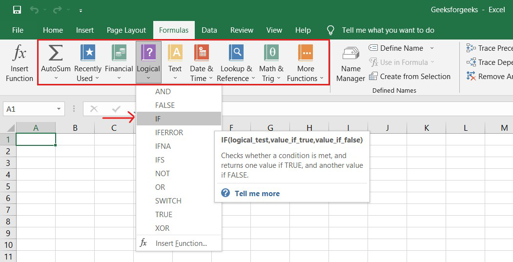
This horizontal menu, shown below, in more recent versions of Excel allows you to find and insert Excel formulas into specific cells of your spreadsheet. On the Formulas tab, you can find all available Excel functions in the Function Library:

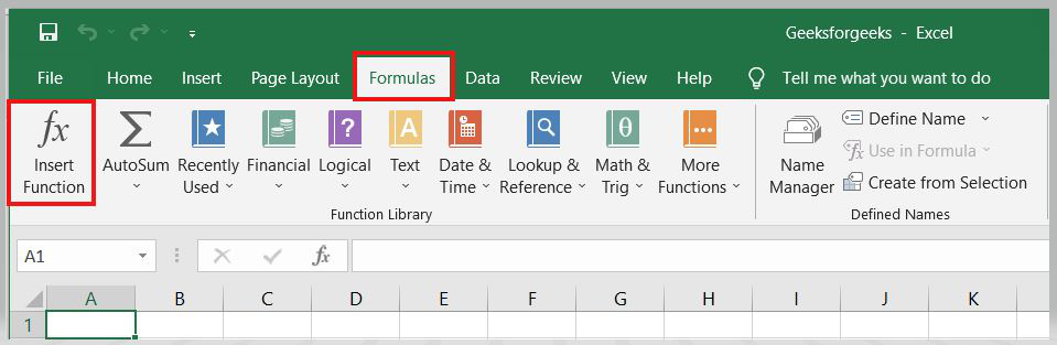
The more you use Excel formulas, the easier it will be to remember and perform them manually. Excel has over 400 functions, and the number is increasing from version to version. The formulas can be inserted into Excel using the following method:

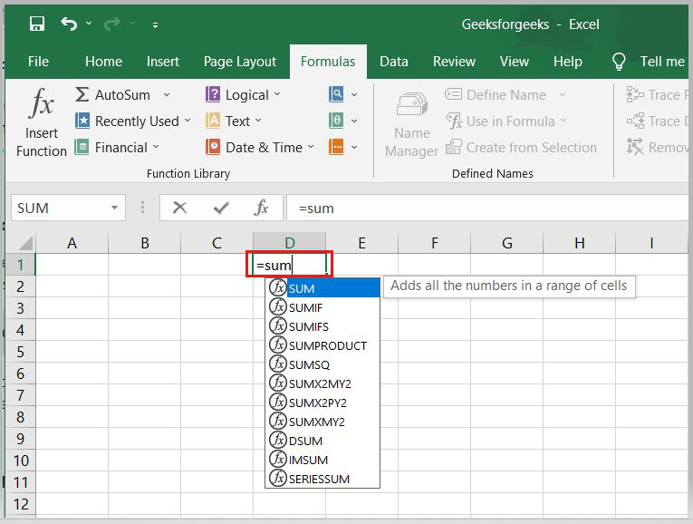
1. Simple insertion of the formula(Typing a formula in the cell):

Typing a formula into a cell or the formula bar is the simplest way to insert basic Excel formulas. Typically, the process begins with typing an equal sign followed by the name of an Excel function. Excel is quite intelligent in that it displays a pop-up function hint when you begin typing the name of the function.

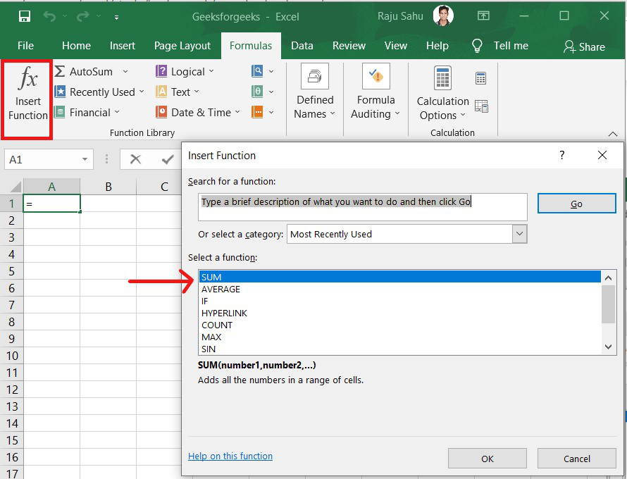
2. Using the Insert Function option on the Formulas Tab:

If you want complete control over your function insertion, use the Excel Insert Function dialogue box. To do so, go to the Formulas tab and select the first menu, Insert Function. All the functions will be available in the dialogue box.

3. Choosing a Formula from One of the Formula Groups in the Formula Tab:

This option is for those who want to quickly dive into their favorite functions. Navigate to the Formulas tab and select your preferred group to access this menu. Click to reveal a sub-menu containing a list of functions. You can then choose your preference. If your preferred group isn’t on the tab, click the More Functions option — it’s most likely hidden there.

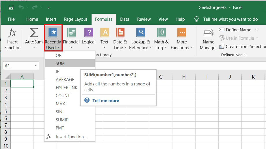
4. Use Recently Used Tabs for Quick Insertion:

If retyping your most recent formula becomes tedious, use the Recently Used menu. It’s on the Formulas tab, the third menu option after AutoSum.

Basic Excel Formulas and Functions:

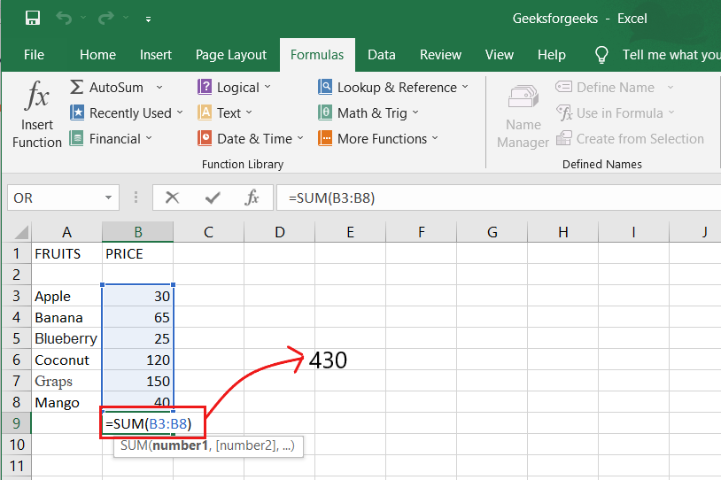
1. SUM:

The SUM formula in Excel is one of the most fundamental formulas you can use in a spreadsheet, allowing you to calculate the sum (or total) of two or more values. To use the SUM formula, enter the values you want to add together in the following format: =SUM(value 1, value 2,…..).

Example: In the below example to calculate the sum of price of all the fruits, in B9 cell type =SUM(B3:B8). this will calculate the sum of B3, B4, B5, B6, B7, B8 Press “Enter,” and the cell will produce the sum: 430.

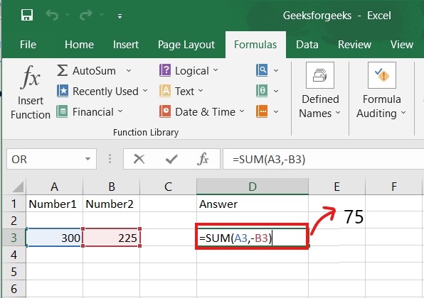
2. SUBTRACTION:

To use the subtraction formula in Excel, enter the cells you want to subtract in the format =SUM (A1, -B1). This will subtract a cell from the SUM formula by appending a negative sign before the cell being subtracted.

For example, if A3 was 300 and B3 was 225, =SUM(A1, -B1) would perform 300 + -225, returning a value of 75 in D3 cell.

3. MULTIPLICATION:

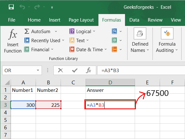
In Excel, enter the cells to be multiplied in the format =A3*B3 to perform the multiplication formula. An asterisk is used in this formula to multiply cell A3 by cell B3.

For example, if A3 was 300 and B3 was 225, =A1*B1 would return a value of 67500.

Highlight an empty cell in an Excel spreadsheet to multiply two or more values. Then, in the format =A1*B1…, enter the values or cells you want to multiply together. The asterisk effectively multiplies each value in the formula.

To return your desired product, press Enter. Take a look at the screenshot above to see how this looks.

4. DIVISION:

To use the division formula in Excel, enter the dividing cells in the format =A3/B3. This formula divides cell A3 by cell B3 with a forward slash, “/.”

For example, if A3 was 300 and B3 was 225, =A3/B3 would return a decimal value of 1.333333333.

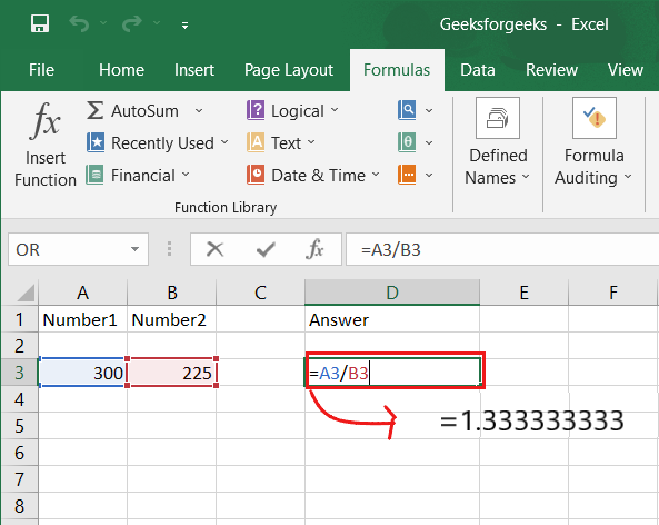
Division in Excel is one of the most basic functions available. To do so, highlight an empty cell, enter an equals sign, “=,” and then the two (or more) values you want to divide, separated by a forward slash, “/.” The output should look like this: =A3/B3, as shown in the screenshot above.

5. AVERAGE:

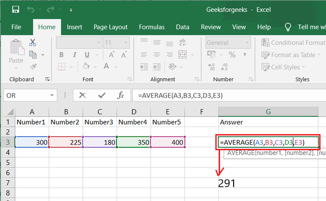
The AVERAGE function finds an average or arithmetic mean of numbers. to find the average of the numbers type = AVERAGE(A3.B3,C3….) and press ‘Enter’ it will produce average of the numbers in the cell.

For example, if A3 was 300, B3 was 225, C3 was 180, D3 was 350, E3 is 400 then =AVERAGE(A3,B3,C3,D3,E3) will produce 291.

6. IF formula:

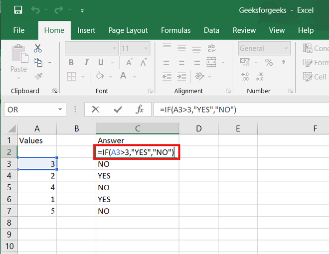
In Excel, the IF formula is denoted as =IF(logical test, value if true, value if false). This lets you enter a text value into a cell “if” something else in your spreadsheet is true or false.

For example, You may need to know which values in column A are greater than three. Using the =IF formula, you can quickly have Excel auto-populate a “yes” for each cell with a value greater than 3 and a “no” for each cell with a value less than 3.

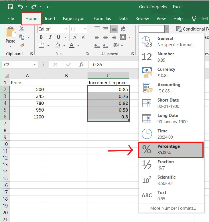
7. PERCENTAGE:

To use the percentage formula in Excel, enter the cells you want to calculate the percentage for in the format =A1/B1. To convert the decimal value to a percentage, select the cell, click the Home tab, and then select “Percentage” from the numbers dropdown.

There isn’t a specific Excel “formula” for percentages, but Excel makes it simple to convert the value of any cell into a percentage so you don’t have to calculate and reenter the numbers yourself.

The basic setting for converting a cell’s value to a percentage is found on the Home tab of Excel. Select this tab, highlight the cell(s) you want to convert to a percentage, and then select Conditional Formatting from the dropdown menu (this menu button might say “General” at first). Then, from the list of options that appears, choose “Percentage.” This will convert the value of each highlighted cell into a percentage. This feature can be found further down.

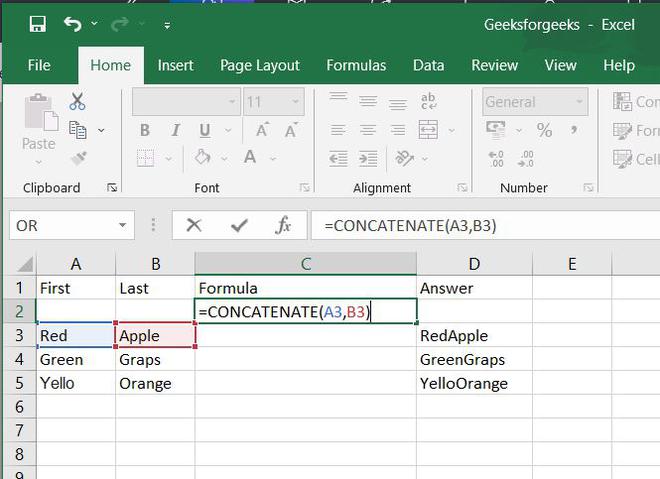
8. CONCATENATE:

CONCATENATE is a useful formula that combines values from multiple cells into the same cell.

For example , =CONCATENATE(A3,B3) will combine Red and Apple to produce RedApple.

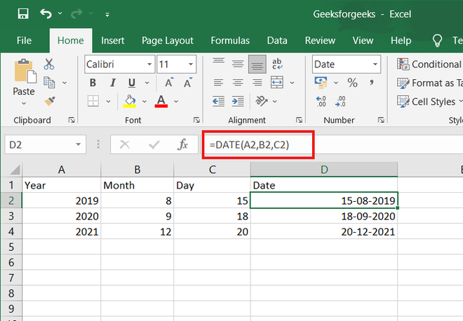
9. DATE:

DATE is the Excel DATE formula =DATE(year, month, day). This formula will return a date corresponding to the values entered in the parentheses, including values referred to from other cells.. For example, if A2 was 2019, B2 was 8, and C1 was 15, =DATE(A1,B1,C1) would return 15-08-2019.

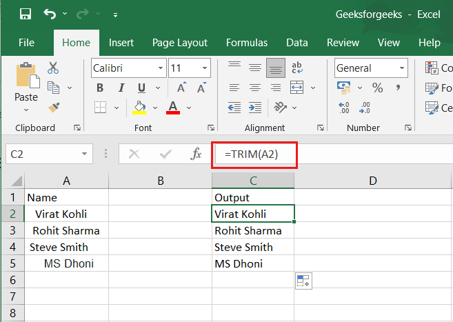
10. TRIM:

The TRIM formula in Excel is denoted =TRIM(text). This formula will remove any spaces that have been entered before and after the text in the cell. For example, if A2 includes the name ” Virat Kohli” with unwanted spaces before the first name, =TRIM(A2) would return “Virat Kohli” with no spaces in a new cell.

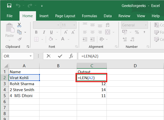
11. LEN:

LEN is the function to count the number of characters in a specific cell when you want to know the number of characters in that cell. =LEN(text) is the formula for this. Please keep in mind that the LEN function in Excel counts all characters, including spaces:

For example,=LEN(A2), returns the total length of the character in cell A2 including spaces.

Источник

How to enter formulas in Excel cells?

How to enter formulas manually?

How to enter formulas using the mouse?

How to enter formulas using the keyboard?

Use AutoSum

Need more help?

Need more help?

Want more options?

About This Article

Is this article up to date?

Write Basic Formulas in Excel

Table of contents

How to Write/Insert Formulas in Excel?

Example #1

Example #2

How to use Built-in Excel Functions?

Example #1 – SUM Function

Example #2 – AVERAGE Function

Things to Remember about Inserting Formula in Excel

Recommended Articles

How to enter a formula in Excel

Creating formulas that refer to other cells in the same worksheet

Creating formulas that refer to cells in other worksheets

Creating formulas that link to other workbooks

Summary

The basics

Entering a spreadsheet formula

Formula examples

=

AVERAGE

COUNT

COUNTA

COUNTIF

IF

INDIRECT

MIN AND MAX

PRODUCT

RAND

RANDBETWEEN

ROUND

SUM

SUMIF

TODAY

TREND

TRIM

VLOOKUP

How to Insert Formulas in Excel?

1. Simple insertion of the formula(Typing a formula in the cell):

2. Using the Insert Function option on the Formulas Tab:

3. Choosing a Formula from One of the Formula Groups in the Formula Tab:

4. Use Recently Used Tabs for Quick Insertion:

Basic Excel Formulas and Functions:

1. SUM:

2. SUBTRACTION:

3. MULTIPLICATION:

4. DIVISION:

5. AVERAGE:

6. IF formula:

7. PERCENTAGE:

8. CONCATENATE:

9. DATE:

10. TRIM:

11. LEN: