
Return to VBA Code Examples
This tutorial will show you how to use the Range.End property in VBA.
Most things that you do manually in an Excel workbook or worksheet can be automated in VBA code.
If you have a range of non-blank cells in Excel, and you press Ctrl+Down Arrow, your cursor will move to the last non-blank cell in the column you are in. Similarly, if you press Ctrl+Up Arrow, your cursor will move to the first non-blank cell. The same applies for a row using the Ctrl+Right Arrow or Ctrl+Left Arrow to go to the beginning or end of that row. All of these key combinations can be used within your VBA code using the End Function.
Range End Property Syntax
The Range.End Property allows you to move to a specific cell within the Current Region that you are working with.
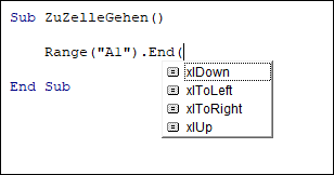
expression.End (Direction)
the expression is the cell address (Range) of the cell where you wish to start from eg: Range(“A1”)
END is the property of the Range object being controlled.
Direction is the Excel constant that you are able to use. There are 4 choices available – xlDown, xlToLeft, xlToRight and xlUp.
Moving to the Last Cell
The procedure below will move you to the last cell in the Current Region of cells that you are in.
Sub GoToLast()
'move to the last cell occupied in the current region of cells
   Range("A1").End(xlDown).Select
End Sub
Counting Rows
The following procedure allows you to use the xlDown constant with the Range End property to count how many rows are in your current region.
Sub GoToLastRowofRange()
   Dim rw As Integer
   Range("A1").Select
'get the last row in the current region
   rw = Range("A1").End(xlDown).Row
'show how many rows are used
   MsgBox "The last row used in this range is " & rw
End Sub
While the one below will count the columns in the range using the xlToRight constant.
Sub GoToLastCellofRange()
   Dim col As Integer
   Range("A1").Select
'get the last column in the current region
   col = Range("A1").End(xlToRight).Column
'show how many columns are used
   MsgBox "The last column used in this range is " & col
 End Sub
Creating a Range Array
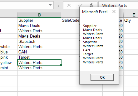
The procedure below allows us to start at the first cell in a range of cells, and then use the End(xlDown) property to find the last cell in the range of cells. We can then ReDim our array with the total rows in the Range, thereby allowing us to loop through the range of cells.
Sub PopulateArray()
'declare the array
   Dim strSuppliers() As String
'declare the integer to count the rows
   Dim n As Integer
'count the rows
   n = Range("B1", Range("B1").End(xlDown)).Rows.Count
'initialise and populate the array
   ReDim strCustomers(n)
'declare the integer for looping
   Dim i As Integer
'populate the array
   For i = 0 To n
     strCustomers(i) = Range("B1").Offset(i, 0).Value
   Next i
'show message box with values of array
   MsgBox Join(strCustomers, vbCrLf)
End Sub
When we run this procedure, it will return the following message box.
VBA Coding Made Easy
Stop searching for VBA code online. Learn more about AutoMacro — A VBA Code Builder that allows beginners to code procedures from scratch with minimal coding knowledge and with many time-saving features for all users!

Learn More!
I was just wondering if you could help me better understand what .Cells(.Rows.Count,"A").End(xlUp).row does. I understand the portion before the .End part.
![]()
asked Nov 21, 2014 at 16:20
![]()
2
It is used to find the how many rows contain data in a worksheet that contains data in the column «A». The full usage is
lastRowIndex = ws.Cells(ws.Rows.Count, "A").End(xlUp).row
Where ws is a Worksheet object. In the questions example it was implied that the statement was inside a With block
With ws
    lastRowIndex = .Cells(.Rows.Count, "A").End(xlUp).row
End With
ws.Rows.Countreturns the total count of rows in the worksheet (1048576 in Excel 2010)..Cells(.Rows.Count, "A")returns the bottom most cell in column «A» in the worksheet
Then there is the End method. The documentation is ambiguous as to what it does.
Returns a Range object that represents the cell at the end of the region that contains the source range
Particularly it doesn’t define what a «region» is. My understanding is a region is a contiguous range of non-empty cells. So the expected usage is to start from a cell in a region and find the last cell in that region in that direction from the original cell. However there are multiple exceptions for when you don’t use it like that:
- If the range is multiple cells, it will use the region of
rng.cells(1,1). - If the range isn’t in a region, or the range is already at the end of the region, then it will travel along the direction until it enters a region and return the first encountered cell in that region.
- If it encounters the edge of the worksheet it will return the cell on the edge of that worksheet.
So Range.End is not a trivial function.
.rowreturns the row index of that cell.
answered Nov 21, 2014 at 16:51
![]()
cheezsteakcheezsteak
2,6924 gold badges22 silver badges38 bronze badges
0
[A1].End(xlUp)
[A1].End(xlDown)
[A1].End(xlToLeft)
[A1].End(xlToRight)
is the VBA equivalent of being in Cell A1 and pressing Ctrl + Any arrow key. It will continue to travel in that direction until it hits the last cell of data, or if you use this command to move from a cell that is the last cell of data it will travel until it hits the next cell containing data.
If you wanted to find that last «used» cell in Column A, you could go to A65536 (for example, in an XL93-97 workbook) and press Ctrl + Up to «snap» to the last used cell. Or in VBA you would write:
Range("A65536").End(xlUp) which again can be re-written as Range("A" & Rows.Count).End(xlUp) for compatibility reasons across workbooks with different numbers of rows.
answered Nov 21, 2014 at 18:13
![]()
SierraOscarSierraOscar
17.4k6 gold badges41 silver badges68 bronze badges
The first part:
.Cells(.Rows.Count,"A")
Sends you to the bottom row of column A, which you knew already.
The End function starts at a cell and then, depending on the direction you tell it, goes that direction until it reaches the edge of a group of cells that have text. Meaning, if you have text in cells C4:E4 and you type:
Sheet1.Cells(4,"C").End(xlToRight).Select
The program will select E4, the rightmost cell with text in it.
In your case, the code is spitting out the row of the very last cell with text in it in column A. Does that help?
answered Nov 21, 2014 at 16:44
![]()
rpalorpalo
2431 silver badge13 bronze badges
.Cells(.Rows.Count,"A").End(xlUp).row
I think the first dot in the parenthesis should not be there, I mean, you should write it in this way:
.Cells(Rows.Count,"A").End(xlUp).row
Before the Cells, you can write your worksheet name, for example:
Worksheets("sheet1").Cells(Rows.Count, 2).End(xlUp).row
The worksheet name is not necessary when you operate on the same worksheet.
![]()
Jason D
7,84510 gold badges35 silver badges39 bronze badges
answered Sep 13, 2015 at 18:24
![]()
0
In VBA, when we have to find the last row, there are many different methods. The most commonly used method is the End(XLDown) method. Other methods include finding the last value using the find function in VBA, End(XLDown). The row is the easiest way to get to the last row.
Excel VBA Last Row
If writing the code is your first progress in VBA, then making the code dynamic is your next step. Excel is full of cell referencesCell reference in excel is referring the other cells to a cell to use its values or properties. For instance, if we have data in cell A2 and want to use that in cell A1, use =A2 in cell A1, and this will copy the A2 value in A1.read more. The moment we refer to the cell, it becomes fixed. If our data increases, we need to go back to the cell reference and change the references to make the result up to date.
For an example, look at the below code.
Code:
Sub Last_Row_Example1()

   Range("D2").Value = WorksheetFunction.Sum(Range("B2:B7"))

End Sub

The above code says in D2 cell value should be the summation of Range (“B2:B7”).
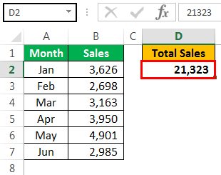
Now, we will add more values to the list.

Now, if we run the code, it will not give us the updated result. Rather, it still sticks to the old range, i.e., Range (“B2: B7”).
That is where dynamic code is very important.
Finding the last used row in the column is crucial in making the code dynamic. This article will discuss finding the last row in Excel VBA.
Table of contents
- Excel VBA Last Row
- How to Find Last Used Row in the Column?
- Method #1
- Method #2
- Method #3
- Recommended Articles
- How to Find Last Used Row in the Column?
How to Find the Last Used Row in the Column?
Below are the examples to find the last used row in Excel VBA.
You can download this VBA Last Row Template here – VBA Last Row Template
Method #1
Before we explain the code, we want you to remember how you go to the last row in the normal worksheet.
We will use the shortcut key Ctrl + down arrow.
It will take us to the last used row before any empty cell. We will also use the same VBA method to find the last row.
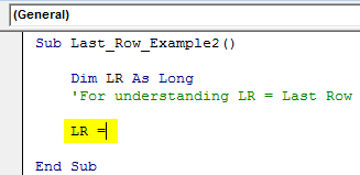
Step 1: Define the variable as LONG.
Code:
Sub Last_Row_Example2()

   Dim LR As Long
   'For understanding LR = Last Row
End Sub

Step 2: We will assign this variable’s last used row number.
Code:
Sub Last_Row_Example2()

   Dim LR As Long
   'For understanding LR = Last Row

   LR =

End Sub
Step 3: Write the code as CELLS (Rows.Count,
Code:
Sub Last_Row_Example2()

   Dim LR As Long
   'For understanding LR = Last Row

   LR = Cells(Rows.Count,

End Sub

Step 4: Now, mention the column number as 1.
Code:
Sub Last_Row_Example2()

   Dim LR As Long
   'For understanding LR = Last Row
   LR = Cells(Rows.Count, 1)

End Sub
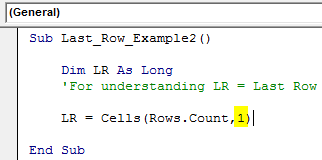
CELLS(Rows.Count, 1) means counting how many rows are in the first column.
So, the above VBA code will take us to the last row of the Excel sheet.
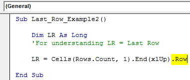
Step 5: If we are in the last cell of the sheet to go to the last used row, we will press the Ctrl + Up Arrow keys.
In VBA, we need to use the end key and up, i.e., End VBA xlUpVBA XLUP is a range and property method for locating the last row of a data set in an excel table. This snippet works similarly to the ctrl + down arrow shortcut commonly used in Excel worksheets.read more
Code:
Sub Last_Row_Example2()

   Dim LR As Long
   'For understanding LR = Last Row

   LR = Cells(Rows.Count, 1).End(xlUp)

End Sub

Step 6: It will take us to the last used row from the bottom. Now, we need the row number of this. So, use the property ROW to get the row number.
Code:
Sub Last_Row_Example2()

  Dim LR As Long
  'For understanding LR = Last Row

  LR = Cells(Rows.Count, 1).End(xlUp).Row

End Sub
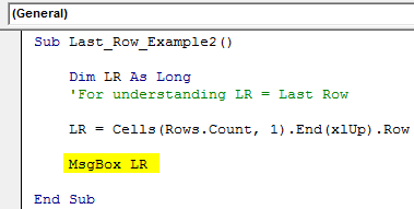
Step 7: Now, the variable holds the last used row number. Show the value of this variable in the message box in the VBA codeVBA MsgBox function is an output function which displays the generalized message provided by the developer. This statement has no arguments and the personalized messages in this function are written under the double quotes while for the values the variable reference is provided.read more.
Code:
Sub Last_Row_Example2()

  Dim LR As Long
  'For understanding LR = Last Row

  LR = Cells(Rows.Count, 1).End(xlUp).Row

  MsgBox LR

End Sub
Run this code using the F5 key or manually. It will display the last used row.

Output:
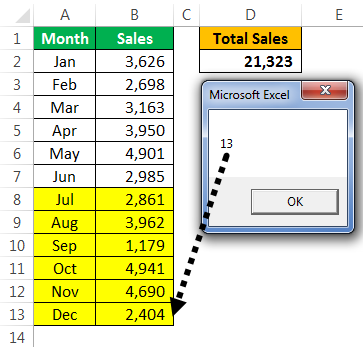
The last used row in this worksheet is 13.
Now, we will delete one more line, run the code, and see the dynamism of the code.

Now, the result automatically takes the last row.
That is what the dynamic VBA last row code is.
As we showed in the earlier example, change the row number from a numeric value to LR.
Code:
Sub Last_Row_Example2()

   Dim LR As Long
   'For understanding LR = Last Row

    LR = Cells(Rows.Count, 1).End(xlUp).Row

    Range("D2").Value = WorksheetFunction.Sum(Range("B2:B" & LR))

End Sub
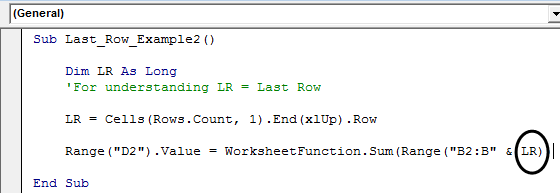
We have removed B13 and added the variable name LR.
Now, it does not matter how many rows you add. It will automatically take the updated reference.
Method #2
We can also find the last row in VBA using the Range objectRange is a property in VBA that helps specify a particular cell, a range of cells, a row, a column, or a three-dimensional range. In the context of the Excel worksheet, the VBA range object includes a single cell or multiple cells spread across various rows and columns.read more and special VBA cells propertyCells are cells of the worksheet, and in VBA, when we refer to cells as a range property, we refer to the same cells. In VBA concepts, cells are also the same, no different from normal excel cells.read more.
Code:
Sub Last_Row_Example3()

   Dim LR As Long

   LR = Range("A:A").SpecialCells(xlCellTypeLastCell).Row

   MsgBox LR
End Sub

The code also gives you the last used row. For example, look at the below worksheet image.

If we run the code manually or use the F5 key result will be 12 because 12 is the last used row.

Output:

Now, we will delete the 12th row and see the result.

Even though we have deleted one row, it still shows the result as 12.
To make this code work, we must hit the “Save” button after every action. Then this code will return accurate results.
We have saved the workbook and now see the result.

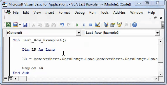
Method #3
We can find the VBA last row in the used range. For example, the below code also returns the last used row.
Code:
Sub Last_Row_Example4()

   Dim LR As Long

   LR = ActiveSheet.UsedRange.Rows(ActiveSheet.UsedRange.Rows.Count).Row

   MsgBox LR
End Sub

It will also return the last used row.
Output:

Recommended Articles
This article has been a guide to VBA Last Row. Here, we learn the top 3 methods to find the last used row in a given column, along with examples and downloadable templates. Below are some useful articles related to VBA: –
- How to Record Macros in VBA Excel?
- Create VBA Loops
- ListObjects in VBA
Хитрости »
1 Май 2011 403611 просмотров
Очень часто при внесении данных на лист Excel возникает вопрос определения последней заполненной или первой пустой ячейки. Чтобы впоследствии с этой первой пустой ячейки начать заносить данные. В этой теме я опишу несколько способов определения последней заполненной ячейки.
В качестве переменной, которой мы будем присваивать номер последней заполненной строки, у нас во всех примерах будет lLastRow. Объявлять мы её будем как Long. Для экономии памяти можно было бы использовать и тип Integer, но т.к. строк на листе может быть больше 32767(это максимальное допустимое значение переменных типа Integer) нам понадобиться именно Long, во избежание ошибки. Подробнее про типы переменных можно прочитать в статье Что такое переменная и как правильно её объявить
Одинаковые переменные для всех примеров
Во всех примерах ниже мы будем запоминать номер последней строки или столбца в одни и те же переменные:
    Dim lLastRow As Long
    'а для lLastCol можно было бы применить и тип Integer,
    'т.к. столбцов в Excel пока меньше 32767, но для однообразности назначим тоже Long
    Dim lLastCol As Long
Способ 1:
Определение
последней заполненной строки
через свойство End
    lLastRow = Cells(Rows.Count,1).End(xlUp).Row
    'или
    lLastRow = Cells(Rows.Count, "A").End(xlUp).Row
1 или «A» — это номер или имя столбца, последнюю заполненную ячейку в котором мы определяем. По сути обе приведенные строки дадут абсолютно одинаковый результат. Просто иногда удобнее указать номер столбца, а иногда его имя. Поэтому использовать можно любой из приведенных вариантов, в зависимости от ситуации.
Определение последнего столбца через свойство End
lLastCol = Cells(1, Columns.Count).End(xlToLeft).Column
1 — это номер строки, последнюю заполненную ячейку в которой мы определяем.
Данный метод определения последней строки/столбца самый распространенный. Используя его мы можем определить последнюю ячейку только в одном конкретном столбце(или строке). В большинстве случаев этого более чем достаточно.
Метод основан именно на принципе работы свойства End. На примере поиска последней строки опишу принцип так, как бы мы это делали руками через выделение ячеек на листе:
- выделили самую последнюю ячейку столбца А на листе(для Excel 2007 и выше это А1048576, а для Excel 2003 — А65536)
- и выполнили переход вверх комбинацией клавиш Ctrl+стрелка вверх. Данная комбинация заставляет Excel двигаться вверх(если точнее, то в направлении стрелки, нажатой вместе с Ctrl) до тех пор, пока не встретиться первая ячейка с формулой или значением. А в случае, если сочетание было вызвано из уже заполненных ячеек — то до первой пустой. И как только Excel доходит до этой ячейки — он её выделяет
- А через свойство .Row мы просто получаем номер строки этой выделенной ячейки
Нюансы:
- даже если в ячейке нет видимого значения, но есть формула — End посчитает ячейку не пустой. С одной стороны вполне справедливо. Но иногда нам надо определить именно «визуально» заполненные ячейки. Поиск ячеек при подобных условиях будет описан ниже(Способ 4: Определение последней ячейки через метод Find)
- если на листе заполнены все строки в просматриваемом столбце(или будут заполнены несколько последних ячеек столбца или даже только одна последняя) — то результат может быть неверный(ну или не совсем такой, какой ожидали)
- Данный способ игнорирует строки, скрытые фильтром, группировкой или командой Скрыть (Hide). Т.е. если последняя строка таблицы будет скрыта, то данный метод вернет номер последней видимой заполненной строки, а не последней реально заполненной.
Ну а если надо получить первую пустую ячейку на листе(а не первую заполненную) — придется вспомнить математику. Т.к. последнюю заполненную мы определили, то первая пустая — следующая за ней. Т.е. к результату необходимо прибавить 1. Это хоть и очевидно, но на всякий случай все же лучше об этом напомнить.
Способ 2:
Определение
последней заполненной строки
через SpecialCells
lLastRow = Cells.SpecialCells(xlLastCell).Row
Определение последнего столбца через SpecialCells
lLastCol = Cells.SpecialCells(xlLastCell).Column
Данный метод не требует указания номера столбца и возвращает последнюю ячейку(Row — строку, Column — столбец).
Если хотите получить номер первой пустой строки или столбца на листе — к результату необходимо прибавить 1.
Нюансы:
- Используя данный способ следует помнить, что не всегда можно получить реальную последнюю заполненную ячейку, т.е. именно ячейку со значением. Метод SpecialCells определяет самую «дальнюю» ячейку на листе, используя при этом механизм «запоминания» тех ячеек, в которых мы работали в данном листе. Т.е. если мы занесем в ячейку AZ90345 значение и сразу удалим его — lLastRow, полученная через SpecialCells будет равна значению именно этой ячейки, из которой вы только что удалили значения(т.е. 90345). Другими словами требует обязательного обновления данных, а этого можно добиться только сохранив файла, а временами даже только закрыв файл и открыв его снова. Так же, если какая-либо ячейка содержит форматирование(например, заливку), но не содержит никаких значений, то метод SpecialCells посчитает её используемой и будет учитывать как заполненную.
Этот недостаток можно попробовать обойти, вызвав перед определением последней ячейки вот такую строку кода:With ActiveSheet.UsedRange: End With
Это должно переопределить границы рабочего диапазона и тогда определение последней строки/столбца сработает как ожидается, даже если до этого в ячейке содержались данные, которые впоследствии были удалены.
Выглядеть в единой процедуре это будет так:Sub GetLastCell() Dim lLastRow As Long 'переопределяем рабочий диапазон листа With ActiveSheet.UsedRange: End With 'ищем последнюю заполненную ячейку на листе lLastRow = Cells.SpecialCells(xlLastCell).Row End Sub
- даже если в ячейке нет видимого значения, но есть формула — SpecialCells посчитает ячейку не пустой
- Данный метод определения последней ячейки не будет работать на защищенном листе(Рецензирование(Review) —Защитить лист(Protect Sheet)).
- Данный метод не будет работать при использовании внутри UDF. Точнее будет работать не так, как ожидается. Подробнее про некоторые «баги» работы встроенных методов внутри UDF(функций пользователя) я описывал в этой статье: Глюк работы в UDF методов SpecialCells и FindNext
Сам же я этот метод обычно использую для определения последней ячейки в только что созданном файле, в котором только добавляю строки кодом и в котором не может быть описанных выше нюансов.
Способ 3:
Определение последней строки через UsedRange
lLastRow = ActiveSheet.UsedRange.Row + ActiveSheet.UsedRange.Rows.Count - 1
Определение последнего столбца через UsedRange
lLastCol = ActiveSheet.UsedRange.Column + ActiveSheet.UsedRange.Columns.Count - 1
НЕМНОГО ПОЯСНЕНИЙ:
- ActiveSheet.UsedRange.Row — этой строкой мы определяем первую ячейку, с которой начинаются данные на листе. Важно понимать для чего это — если у вас первые строк 5 не заполнены ничем(т.е. самые первые данные заносились начиная с 6-ой строки листа), то ActiveSheet.UsedRange.Row вернет именно 6(т.е. номер первой строки с данными). Если же все строки заполнены — то вернет 1.
- ActiveSheet.UsedRange.Rows.Count — определяем кол-во строк, входящих в весь диапазон данных на листе. При этом неважно, есть ли данные в ячейках или нет — достаточно было поработать в этих ячейках и удалить значения или просто изменить цвет заливки.
В итоге получается: первая строка данных + кол-во строк с данными — 1. Зачем вычитать единицу? Попробуем посчитать вместе: первая строка: 6. Всего строк: 3. 6 + 3 = 9. Вроде все верно. А теперь выделим на листе три ячейки, начиная с 6-ой. Выделение завершилось на 8-ой строке. Потому что в 6-ой строке уже есть данные. Поэтому и надо вычесть 1, чтобы учесть этот момент. Думаю, не надо пояснять, что если надо получить первую пустую ячейку — можно 1 не вычитать
- То же самое и с ActiveSheet.UsedRange.Column, только уже не для строк, а для столбцов.

Нюансы:
- Обладает некоторыми недостатками предыдущего метода. Определяет самую «дальнюю» ячейку на листе, используя при этом механизм «запоминания» тех ячеек, в которых мы работали в данном листе. Следовательно попробовать обойти этот момент можно точно так же: перед определением последней строки/столбца записать строку: With ActiveSheet.UsedRange: End With
Это должно переопределить границы рабочего диапазона и тогда определение последней строки/столбца сработает как ожидается, даже если до этого в ячейке содержались данные, которые впоследствии были удалены. - даже если в ячейке нет видимого значения, но есть формула — UsedRange посчитает ячейку не пустой
Однако метод через UsedRange.Row работает прекрасно и при установленной на лист защите и внутри UDF, что делает его более предпочтительным, чем метод через SpecialCells при равных условиях.
Способ 4:
Определение последней строки и столбца, а так же адрес ячейки методом Find
Sub GetLastCell_Find()
    Dim rF As Range
    Dim lLastRow As Long, lLastCol As Long
    'ищем последнюю ячейку на листе, в которой хранится хоть какое-то значение
    Set rF = ActiveSheet.UsedRange.Find(What:="*", LookIn:=xlValues, LookAt:=xlWhole, SearchDirection:=xlPrevious, MatchCase:=False, MatchByte:=False)
    If Not rF Is Nothing Then
        lLastRow = rF.Row    'последняя заполненная строка
        lLastCol = rF.Column 'последний заполненный столбец
        MsgBox rF.Address 'показываем сообщение с адресом последней ячейки
    Else
        'если ничего не нашлось - значит лист пустой
        'и можно назначить в качестве последних первую строку и столбец
        lLastRow = 1
        lLastCol = 1
        MsgBox "A1" 'показываем сообщение с адресом ячейки А1
    End If
End Sub
Этот метод, пожалуй, самый оптимальный в случае, если надо определить последнюю строку/столбец на листе без учета форматов и формул — только по отображаемому значению в ячейке. Например, если на листе большая таблица и последние строки заполнены формулами, возвращающими при определенных условиях пустую ячейку(=ЕСЛИ(A1>0;1;»»)), предыдущие варианты вернут строку/столбец ячейки с последней ячейкой, в которой формула. В то время как данный метод вернет адрес ячейки только в случае, если в ячейке реально отображается какое-то значение. Такой подход часто используется для того, чтобы определить границы данных для последующего анализа заполненных данных, чтобы не захватывать пустые ячейки с формулами и не тратить время на их проверку.
Здесь следует обратить внимание на параметры метода Find. В данном случае мы специально указываем искать по значениям, а не по формулам:
Set rF = ActiveSheet.UsedRange.Find(What:=»*», LookIn:=xlValues, LookAt:=xlWhole, SearchDirection:=xlPrevious, MatchCase:=False, MatchByte:=False)
Нюансы:
- Метод Find, вызванный с листа или другим кодом, имеет свойство запоминать все параметры последнего поиска, а если поиск еще не вызывался — то применяются параметры по умолчанию. А по умолчанию поиск идет всегда по формулам. Поэтому я настоятельно рекомендую указывать принудительно все необходимые параметры, как в примере.
- Метод Find не будет учитывать в просмотре скрытые строки и столбцы. Это следует учитывать при его применении.
Пара небольших практических кодов
Коды ниже могут помочь понять, как использовать приведенные выше строки кода по поиску последней ячейки/строки:
Sub GetLastCell()
    Dim lLastRow As Long
    Dim lLastCol As Long
    'определили последнюю заполненную ячейку с учетом формул в столбце А
    lLastRow = Cells(Rows.Count, 1).End(xlUp).Row
    MsgBox "Заполненные ячейки в столбце А: " & Range("A1:A" & lLastRow).Address
    'определили последний заполненный столбец на листе(с учетом формул и форматирования)
    lLastCol = Cells.SpecialCells(xlLastCell).Column
    MsgBox "Заполненные ячейки в первой строке: " & Range(Cells(1, 1), Cells(1, lLastCol)).Address
    'выводим сообщение с адресом последней ячейки на листе(с учетом формул и форматирования)
    MsgBox "Адрес последней ячейки диапазона на листе: " & Cells.SpecialCells(xlLastCell).Address
End Sub
Выделяем диапазон ячеек в столбцах с А по С, определяя последнюю ячейку по столбцу A этого же листа:
Sub SelectToLastCell()
    Range("A1:C" & Cells(Rows.Count, 1).End(xlUp).Row).Select
End Sub
Копируем ячейку B1 в первую пустую ячейку столбца A этого же листа:
Sub CopyToFstEmptyCell()
    Dim lLastRow As Long
    lLastRow = Cells(Rows.Count, 1).End(xlUp).Row 'определили последнюю заполненную ячейку
    Range("B1").Copy Cells(lLastRow+1, 1)         'скопировали В1 и вставили в следующую после определенной ячейки
End Sub
А код ниже делает тоже самое, но одной строкой — применяется Offset и используется тот факт, что изначально методом End мы получаем именно ячейку, а не номер строки(номер строки мы получаем позже через свойство .Row):
Sub CopyToFstEmptyCell()
    Range("B1").Copy Destination:=Cells(Rows.Count, 1).End(xlUp).Offset(1)
End Sub
Range(«B1»).Copy — копирует ячейку В1. Если для аргумента Destination указать другую ячейку, то в неё будет вставлена скопированная ячейка. Мы передаем в этот аргумент определенную методом End ячейку
Cells(Rows.Count, 1).End(xlUp) — возвращает последнюю заполненную ячейку в столбце А (не строку, а именно ячейку)
Offset(1) — смещает полученную ячейку на строку вниз
Используем инструмент автозаполнение(протягивание) столбца В, начиная с ячейки B2 и определяя последнюю ячейку для заполнения на основании столбца А
Sub AutoFill_B()
    Dim lLastRow As Long
    lLastRow = Cells(Rows.Count, 1).End(xlUp).Row
    Range("B2").AutoFill Destination:=Range("B2:B" & lLastRow)
End Sub
На самом деле практических кодов может быть куда больше, т.к. определение последней заполненной или первой пустой ячейки является чуть ли не самой распространенной задачей при написании кодов в Excel.
Так же см.:
Как получить последнюю заполненную ячейку формулой?
Как определить первую заполненную ячейку на листе?
Что такое переменная и как правильно её объявить?
Статья помогла? Поделись ссылкой с друзьями!
![]() Видеоуроки
Видеоуроки
Поиск по меткам
Access
apple watch
Multex
Power Query и Power BI
VBA управление кодами
Бесплатные надстройки
Дата и время
Записки
ИП
Надстройки
Печать
Политика Конфиденциальности
Почта
Программы
Работа с приложениями
Разработка приложений
Росстат
Тренинги и вебинары
Финансовые
Форматирование
Функции Excel
акции MulTEx
ссылки
статистика
Свойство End объекта Range применяется для поиска первых и последних заполненных ячеек в VBA Excel — аналог сочетания клавиш Ctrl+стрелка.
Свойство End объекта Range возвращает объект Range, представляющий ячейку в конце или начале заполненной значениями области исходного диапазона по строке или столбцу в зависимости от указанного направления. Является в VBA Excel программным аналогом сочетания клавиш — Ctrl+стрелка (вверх, вниз, вправо, влево).
Возвращаемая свойством Range.End ячейка в зависимости от расположения и содержания исходной:
| Исходная ячейка | Возвращаемая ячейка |
|---|---|
| Исходная ячейка пустая | Первая заполненная ячейка или, если в указанном направлении заполненных ячеек нет, последняя ячейка строки или столбца в заданном направлении. |
| Исходная ячейка не пустая и не крайняя внутри исходного заполненного диапазона в указанном направлении | Последняя заполненная ячейка исходного заполненного диапазона в указанном направлении |
| Исходная ячейка не пустая, но в указанном направлении является крайней внутри исходного заполненного диапазона | Первая заполненная ячейка следующего заполненного диапазона или, если в указанном направлении заполненных ячеек нет, последняя ячейка строки или столбца в заданном направлении. |
Синтаксис
|
Expression.End (Direction) |
Expression — выражение (переменная), представляющее объект Range.
Параметры
| Параметр | Описание |
|---|---|
| Direction | Константа из коллекции XlDirection, задающая направление перемещения. Обязательный параметр. |
Константы XlDirection:
| Константа | Значение | Направление |
|---|---|---|
| xlDown | -4121 | Вниз |
| xlToLeft | -4159 | Влево |
| xlToRight | -4161 | Вправо |
| xlUp | -4162 | Вверх |
Примеры
Скриншот области рабочего листа для визуализации примеров применения свойства Range.End:

Примеры возвращаемых ячеек свойством End объекта Range("C10") с разными значениями параметра Direction:
| Выражение с Range.End | Возвращенная ячейка |
|---|---|
Set myRange = Range("C10").End(xlDown) |
Range("C16") |
Set myRange = Range("C10").End(xlToLeft) |
Range("A10") |
Set myRange = Range("C10").End(xlToRight) |
Range("E10") |
Set myRange = Range("C10").End(xlUp) |
Range("C4") |
Пример возвращения заполненной значениями части столбца:
|
Sub Primer() Dim myRange As Range Set myRange = Range(Range(«C10»), Range(«C10»).End(xlDown)) MsgBox myRange.Address ‘Результат: $C$10:$C$16 End Sub |
VBA Last Row or Column with Data
It is important to know how to generate a code that identifies the address of the last row or column with data from a spreadsheet. It is useful as a final counter in Loops and as a reference for intervals.
VBA Count
The .Count property, when used for a Range object, returns the number of cells in a given range. (whether they are filled or not).
MsgBox Range("A1:B7").Count 'Returns 14
If you want to know the number of columns or of rows of a given range, you can use the Columns or the Rows properties in conjunction with the Count property.
    MsgBox Range("A1:B7").Rows.Count    'Returns 7
    MsgBox Range("A1:B7").Columns.Count 'Returns 2
The .Count property returns the number of objects of a given collection.
If you want to know the number of rows or columns in the worksheet, you can use Rows or Columns without specifying the cells with the Range:
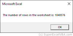
MsgBox "The number of rows in the worksheet is: " & Rows.Count
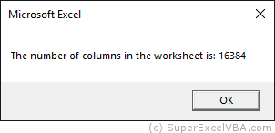
MsgBox "The number of columns in the worksheet is: " & Columns.Count
VBA End
Although the Count property is very useful, it returns only the available amount of elements, even if they are without values.
The End property, used in conjunction with the Range object, will return the last cell with content in a given direction. It is equivalent to pressing
 +
+
( or
or
 or
or
 or
or
 ).
).
    Range("A1").End(xlDown).Select
    'Range("A1").End([direction]).Select
When using End it is necessary to define its argument, the direction: xlUp, xlToRight, xlDown, xlToLeft.
You can also use the end of the worksheet as reference, making it easy to use the xlUp argument:
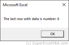
MsgBox "The last row with data is number: " & Cells(Rows.Count, 1).End(xlUp).Row
VBA Last Cell Filled
Note that there are some ways to determine the last row or column with data from a spreadsheet:
    Range("A1").End(xlDown).Row
    'Determines the last row with data from the first column

    Cells(Rows.Count, 1).End(xlUp).Row
    'Determines the last row with data from the first column

    Range("A1").End(xlToRight).Column
    'Determines the last column with data from the first row

    Cells(1,Columns.Count).End(xlToLeft).Column
    'Determines the last column with data from the first row
Show Advanced Topics
Consolidating Your Learning
Suggested Exercises
SuperExcelVBA.com is learning website. Examples might be simplified to improve reading and basic understanding. Tutorials, references, and examples are constantly reviewed to avoid errors, but we cannot warrant full correctness of all content. All Rights Reserved.
Excel ® is a registered trademark of the Microsoft Corporation.
© 2023 SuperExcelVBA | ABOUT
![]()
Finding last used row and column is one of the basic and important task for any automation in excel using VBA. For compiling sheets, workbooks and arranging data automatically, you are required to find the limit of the data on sheets.
This article will explain every method of finding last row and column in excel in easiest ways.
1. Find Last Non-Blank Row in a Column using Range.End
Let’s see the code first. I’ll explain it letter.
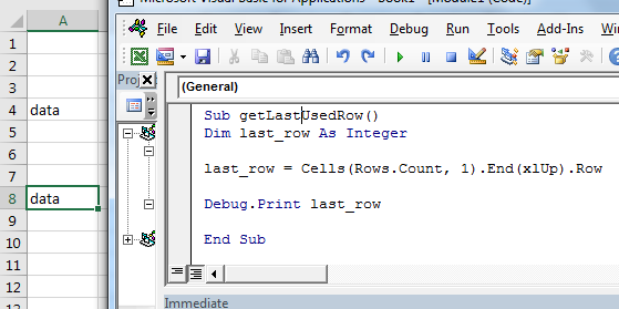
Sub getLastUsedRow()

    Dim last_row As Integer

    last_row = Cells(Rows.Count, 1).End(xlUp).Row ‘This line gets the last row

    Debug.Print last_row

End Sub
The the above sub finds the last row in column 1.
How it works?
It is just like going to last row in sheet and then pressing CTRL+UP shortcut.
Cells(Rows.Count, 1): This part selects cell in column A. Rows.Count gives 1048576, which is usually the last row in excel sheet.
Cells(1048576, 1)
.End(xlUp): End is an method of range class which is used to navigate in sheets to ends. xlUp is the variable that tells the direction. Together this command selects the last row with data.
Cells(Rows.Count, 1).End(xlUp)
.Row : row returns the row number of selected cell. Hence we get the row number of last cell with data in column A. in out example it is 8.
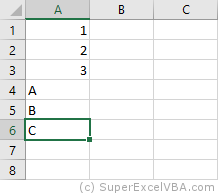
See how easy it is to find last rows with data. This method will select last row in data irrespective of blank cells before it. You can see that in image that only cell A8 has data. All preceding cells are blank except A4.
Select the last cell with data in a column
If you want to select the last cell in A column then just remove “.row” from end and write .select.
Sub getLastUsedRow()

Cells(Rows.Count, 1).End(xlUp).Select ‘This line selects the last cell in a column

End Sub
The “.Select” command selects the active cell.
Get last cell’s address column
If you want to get last cell’s address in A column then just remove “.row” from end and write .address.
Sub getLastUsedRow()

add=Cells(Rows.Count, 1).End(xlUp).address ‘This line selects the last cell in a column
Debug.print add
End Sub
The Range.Address function returns the activecell’s address.
Find Last Non-Blank Column in a Row
It is almost same as finding last non blank cell in a column. Here we are getting column number of last cell with data in row 4.
Sub getLastUsedCol()

    Dim last_col As Integer

    last_col = Cells(4,Columns.Count).End(xlToLeft).Column ‘This line gets the last column

    Debug.Print last_col

End Sub
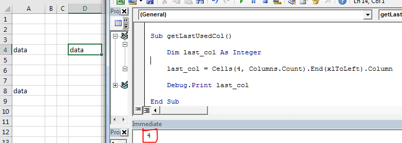
You can see in image that it is returning last non blank cell’s column number in row 4. Which is 4.
How it works?
Well, the mechanics is same as finding last cell with data in a column. We just have used keywords related to columns.
Select Data Set in Excel Using VBA
Now we know, how to get last row and last column of excel using VBA. Using that we can select a table or dataset easily. After selecting data set or table, we can do several operations on them, like copy-paste, formating, deleting etc.
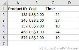
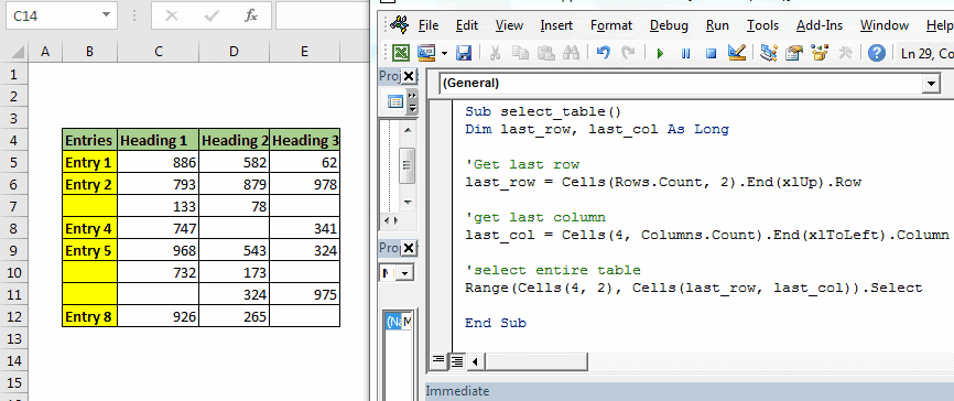
Here we have data set. This data can expand downwards. Only the starting cell is fixed, which is B4. The last row and column is not fixed. We need to select the whole table dynamically using vba.
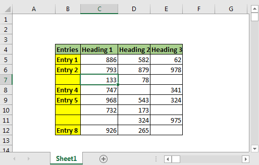
VBA code to select table with blank cells
Sub select_table()
Dim last_row, last_col As Long

'Get last row
last_row = Cells(Rows.Count, 2).End(xlUp).Row

'Get last column
last_col = Cells(4, Columns.Count).End(xlToLeft).Column

'Select entire table
Range(Cells(4, 2), Cells(last_row, last_col)).Select

End Sub
When you run this, entire table will be selected in fraction of a second. You can add new rows and columns. It will always select the entire data.
Benefits of this method:
- It’s easy. We literally wrote only one line to get last row with data. This makes it easy.
- Fast. Less line of code, less time taken.
- Easy to understand.
- Works perfectly if you have clumsy data table with fixed starting point.
Cons of Range.End method:
- The starting point must be know.
- You can only get last non-blank cell in a known row or column. When your starting point is not fixed, it will be useless. Which is very less likely to happen.
2. Find Last Row Using Find() Function
Let’s see the code first.
Sub last_row()

   lastRow = ActiveSheet.Cells.Find("*", searchorder:=xlByRows, searchdirection:=xlPrevious).Row

   Debug.Print lastRow

End Sub

As you can see that in image, that this code returns the last row accurately.
How it works?
Here we use find function to find any cell that contains any thing using wild card operator «*». Asterisk is used to find anything, text or number.
We set search order by rows (searchorder:=xlByRows). We also tell excel vba the direction of search as xlPrevious (searchdirection:=xlPrevious). It makes find function to search from end of the sheet, row wise.

Once it find a cell that contains anything, it stops. We use the Range.Row method to fetch last row from active cell.
Benefits of Find function for getting last cell with data:
- You don’t need to know the starting point. It just gets you last row.
- It can be generic and can be used to find last cell with data in any sheet without any changes.
- Can be used to find any last instance of specific text or number on sheet.
Cons of Find() function:
- It is ugly. Too many arguments.
- It is slow.
- Can’t use to get last non blank column. Technically, you can. But it gets too slow.
3. Using SpecialCells Function To Get Last Row
The SpecialCells function with xlCellTypeLastCell argument returns the last used cell. Lets see the code first
Sub spl_last_row_()
lastRow = ActiveSheet.Cells.SpecialCells(xlCellTypeLastCell).Row
Debug.Print lastRow
End Sub
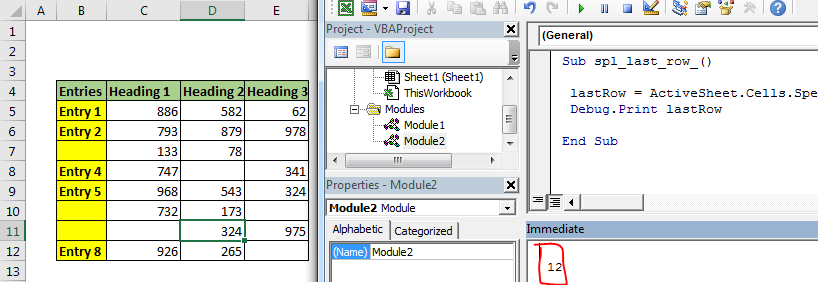
If you run the above code, you will get row number of last used cell.
How it Works?
This is the vba equivalent of shortcut CTRL+End in excel. It selects the last used cell. If record the macro while pressing CTRL+End, you will get this code.
Sub Macro1()
'
' Macro1 Macro
'

'
    ActiveCell.SpecialCells(xlLastCell).Select
End Sub
We just used it to get last used cell’s row number.
Note: As I said above, this method will return the last used cell not last cell with data. If you delete the data in last cell, above vba code will still return the same cells reference, since it was the “last used cell”. You need to save the document first to get last cell with data using this method.
Related Articles:
Delete sheets without confirmation prompts using VBA in Microsoft Excel
Add And Save New Workbook Using VBA In Microsoft Excel 2016
Display A Message On The Excel VBA Status Bar
Turn Off Warning Messages Using VBA In Microsoft Excel 2016
Popular Articles:
The VLOOKUP Function in Excel
COUNTIF in Excel 2016
How to Use SUMIF Function in Excel
Excel VBA Refer to Ranges — Union & Intersect; Resize; Areas, CurrentRegion, UsedRange & End Properties; SpecialCells
An important aspect in vba coding is referencing and using Ranges within a Worksheet. You can refer to or access a worksheet range using properties and methods of the Range object. A Range Object refers to a cell or a range of cells. It can be a row, a column or a selection of cells comprising of one or more rectangular / contiguous blocks of cells. This section (divided into 2 parts) covers various properties and methods for referencing, accessing & using ranges, divided under the following chapters:
Excel VBA Referencing Ranges — Range, Cells, Item, Rows & Columns Properties; Offset; ActiveCell; Selection; Insert:
Range Property, Cells / Item / Rows / Columns Properties, Offset & Relative Referencing, Cell Address;
Activate & Select Cells; the ActiveCell & Selection;
Entire Row & Entire Column Properties, Inserting Cells/Rows/Columns using the Insert Method;
Excel VBA Refer to Ranges — Union & Intersect; Resize; Areas, CurrentRegion, UsedRange & End Properties; SpecialCells:
Ranges — Union & Intersect;
Resize a Range;
Referencing — Contiguous Block(s) of Cells, Range of Contiguous Data, Cells Meeting a Specified Criteria, Used Range, Cell at the End of a Block / Region, Last Used Row or Column;
Related Links:
Working with Objects in Excel VBA
Excel VBA Application Object, the Default Object in Excel
Excel VBA Workbook Object, working with Workbooks in Excel
Microsoft Excel VBA — Worksheets
Excel VBA Custom Classes and Objects
———————————————————————————————————
Contents:
Ranges — Union & Intersect
Resize a Range
Referencing — Contiguous Block(s) of Cells, Range of Contiguous Data, Cells Meeting a Specified Criteria, Used Range, Cell at the End of a Block / Region, Last Used Row or Column
———————————————————————————————————
Ranges — Union & Intersect
Use the Application.Union Method to return a range object representing a union of two or more range objects. Syntax: ApplicationObject.Union(Arg1, Arg2, … Arg29, Arg30). Each argument is a range object and it is necessary to specify atleast 2 range objects as arguments.
Using the union method set the background color of cells B1 & D3 in Sheet1 to red:
Union(Worksheets(«Sheet1»).Cells(1, 2), Worksheets(«Sheet1»).Cells(3, 4)).Interior.Color = vbRed
Using the union method set the background color of 2 named ranges to red:
Union(Range(«NamedRange1»), Range(«NamedRange2»)).Interior.Color = vbRed
Example 8: Using the Union method:
Sub RangeUnion()
Dim rng1 As Range, rng2 As Range, rngUnion As Range
Set rng1 = ActiveWorkbook.Worksheets(«Sheet3»).
Range(«A2:B3»)
Set rng2 = ActiveWorkbook.Worksheets(«Sheet3»).
Range(«C5:D7»)
‘using the union method:
Set rngUnion = Union(rng1, rng2)
‘this will set the background color to red, of cells A2, A3, B2, B3, C5, C6, C7, D5, D6 & D7 in Sheet3 of active workbook:
rngUnion.Interior.Color = vbRed
End Sub
Determining a range which is at the intersection of multiple ranges is a useful tool in vba programming, and is also often used to determine whether the changed range is within or is a part of the specified range in the context of Excel built-in Worksheet_Change Event, wherein a VBA procedure or code gets executed when content of a worksheet cell changes. Using the Application.Intersect Method returns a Range which is at the intersection of two or more ranges. Syntax: ApplicationObject.Intersect(Arg1, Arg2, Arg3, … Arg 30). Specifying the Application object qualifier is optional. Each argument represents the intersecting range and a minimum of two ranges are required to be specified. Refer below examples which explain useing the Intersect method, and also using it in combination with the Union method.
Example 9: Using the Intersect method.
Sub IntersectMethod()
‘examples of using Intersect method
Dim ws As Worksheet
Set ws = Worksheets(«Sheet2»)
‘note that the active cell (used below) can be referred to only in respect of the active worksheet:
ws.Activate
‘—————-
‘If the active cell is within the specified range of A1:B5, its background color will be set to red, however if the active cell is not within the specified range of A1:B5, say the active cell is A10, then you will get a run time error. You can check whether the active cell is within the specified range, as shown below where an If…Then statement is used.
Intersect(ActiveCell, Range(«A1:B5»)).Interior.Color = vbRed
‘—————-
‘If the active cell is not within the specified range of A1:B5, say the active cell is A10, then you will get a run time error. You can check whether the active cell is within the specified range, as shown below where an
If…Then statement is used.
If Intersect(ActiveCell, Range(«A1:B5»)) Is Nothing Then
‘if the active cell is not within the specified range of A1:B5, say the active cell is A10, then below message is returned:
MsgBox «Active Cell does not intersect»
Else
‘if the active cell is within the specified range of A1:B5, say the active cell is A4, then the address «$A$4» will be returned below:
MsgBox Intersect(ActiveCell, Range(«A1:B5»)).Address
‘—————-
‘consider 2 named ranges: «NamedRange8» comprising of range C1:C8 and «NamedRange9» comprising of range A5:E6:
If Intersect(Range(«NamedRange8»), Range(«NamedRange9»)) Is Nothing Then
‘if the ranges do not intersect, then below message will be returned:
MsgBox «Named Ranges do not intersect»
Else
‘in this case, the 2 named ranges intersect, hence the background color of green will be applied to the intersected range of C5:C6:
Intersect(Range(«NamedRange8»), Range(«NamedRange9»)).Interior.Color = vbGreen
End If
End Sub
Example 10: Using Intersect and Union methods in combination — refer Images 6a, 6b, 6c & 6d.
For live code of this example, click to download excel file.
Sub IntersectUnionMethods()
‘using Intersect and Union methods in combination — refer Images 6a, 6b, 6c & 6d.
Dim ws As Worksheet
Dim rng1 As Range, rng2 As Range, cell As Range, rngFinal1 As Range, rngUnion As Range, rngIntersect As Range, rngFinal2 As Range
Dim count As Integer
Set ws = Worksheets(«Sheet1»)
‘set ranges:
Set rng1 = ws.Range(«B1:C10»)
Set rng2 = ws.Range(«A5:D7»)
‘we work on 4 options: (1) cells in rng1 plus cells in rng2; (2) cells common to both rng1 & rng2; (3) cells in rng1 but not in rng2 ie. exclude intersect range from rng1; (4) cells not common to both rng1 & rng2. The first 2 options simply use the Union and Intersect methods respectively. See below.
‘NOTE: each of the 4 below codes need to be run individually.
‘clear background color in worksheet before starting code:
ws.Cells.Interior.ColorIndex = xlNone
‘—————-
‘(1) cells in rng1 plus cells in rng2 — using the Union method, set the background color to red (refer Image 6a):
Union(rng1, rng2).Interior.Color = vbRed
‘—————-
‘(2) cells common to both rng1 & rng2 — using the Intersect method, set the background color to red, of range B5:C7 (refer Image 6b):
If Intersect(rng1, rng2) Is Nothing Then
MsgBox «Ranges do not intersect»
Else
Intersect(rng1, rng2).Interior.Color = vbRed
End If
‘—————-
‘(3) cells in rng1 but not in rng2 ie. exclude intersect range from rng1 — set the background color to red (refer Image 6c):
count = 0
‘check each cell of rng1, and exclude it from final range if it is a part of the intersect range:
For Each cell In rng1
If Intersect(cell, rng2) Is Nothing Then
count = count + 1
‘determine first cell for the final range:
‘instead of «If count = 1 Then» you can alternatively use: «If rngFinal1 Is Nothing Then»
If count = 1 Then
‘include a single (ie. first) cell in the final range:
Set rngFinal1 = cell
Else
‘set final range as union of further matching cells:
Set rngFinal1 = Union(rngFinal1, cell)
End If
End If
Next
rngFinal1.Interior.Color = vbRed
‘—————-
‘(4) cells not common to both rng1 & rng2 ie. exclude intersect area from their union — set the background color to red (refer Image 6d):
Set rngUnion = Union(rng1, rng2)
‘check if intersect range is not empty:
If Not Intersect(rng1, rng2) Is Nothing Then
Set rngIntersect = Intersect(rng1, rng2)
‘check for each cell in the union of both ranges, whether it is also a part of their intersection:
For Each cell In rngUnion
‘if a cell is not part of the intersection of both ranges, then include in the final range:
If Intersect(cell, rngIntersect) Is Nothing Then
‘the first eligible cell for the final range:
If rngFinal2 Is Nothing Then
Set rngFinal2 = cell
Else
Set rngFinal2 = Union(rngFinal2, cell)
End If
End If
Next
‘apply color to the unuion of both ranges excluding their intersect area:
rngFinal2.Interior.Color = vbRed
‘if intersect range is empty:
Else
‘apply color to the union of both ranges if no intersect area:
rngUnion.Interior.Color = vbRed
End If
End Sub
The Intersect method is commonly used with the Excel built-in Worksheet_Change Event (or with the Worksheet_SelectionChange event). You can auto run a VBA code, when content of a worksheet cell changes, with the Worksheet_Change event. The change event occurs when cells on the worksheet are changed. The Intersect method is used to determine whether the changed range is within or is a part of the defined range in this context. Target is a parameter or variable of data type Range ie. Target is a Range Object. It refers to the changed Range and can consist of one or multiple cells. If Target is in the defined Range, and its value or content changes, it will trigger the vba procedure. If Target is not in the defined Range, nothing will happen in the worksheet. The Intersect method is used to determine whether the Target or changed range lies within (or intersects) with the defined range. Note that Worksheet change procedure is installed with the worksheet ie. it must be placed in the code module of the appropriate Sheet object (in the VBE Code window, select «Worksheet» from the left-side «General» drop-down menu and then select «Change» from the right-side «Declarations» drop-down menu). Refer below examples.
Examples of using Intersect method with the worksheet change or selection change events:
Private Sub Worksheet_Change(ByVal Target As Range)
‘Worksheet change procedure is installed with a worksheet ie. it must be placed in the code module of the appropriate Sheet object
‘using Target parameter and Intersect method, with the Worksheet_Change event
‘NOTE: each of the below codes need to be run individually.
‘Using Target Address: if a single cell (A5) value is changed:
If Target.Address = Range(«$A$5»).Address Then MsgBox «A5»
‘Using Target Address: if cell (A1) or cell (A3) value is changed:
If Target.Address = «$A$1» Or Target.Address = «$A$3» Then MsgBox «A1 or A3»
‘Using Target Address: if any cell(s) value other than that of cell (A1) is changed:
If Target.Address <> «$A$1» Then MsgBox «Other than A1»
‘Intersect method for a single cell: If Target intersects with the defined Range of A1 ie. if cell (A1) value is changed:
If Not Intersect(Target, Range(«A1»)) Is Nothing Then MsgBox «A1»
‘At least one cell of Target is within the contiguous range C5:D25:
If Not Intersect(Target, Me.Range(«C5:D25»)) Is Nothing Then MsgBox «C5:D25»
‘At least one cell of Target is in the non-contiguous ranges of A1,B2,C3,E5:F7:
If Not Application.Intersect(Target, Range(«A1,B2,C3,E5:F7»)) Is Nothing Then MsgBox «A1 or B2 or C3 or E5:F7»
End Sub
Private Sub Worksheet_Change(ByVal Target As Range)
‘If you want the code to run if only a single cell in Range(«C1:C10») is changed and do nothing if multiple cells are changed:
If Intersect(Target, Range(«C1:C10»)) Is Nothing Or Target.Cells.count > 1 Then
Exit Sub
Else
MsgBox «Single cell — C1:C10»
End If
End Sub
Private Sub Worksheet_SelectionChange(ByVal Target As Range)
‘example of using Intersect method for worksheet selection change event
Dim rngExclusion As Range
‘set excluded range — no action if excluded range is selected
Set rngExclusion = Union(Range(«A1:B1»), Range(«E1:F1»))
If Not Intersect(Target, rngExclusion) Is Nothing Then Exit Sub
‘convert cell text to lower case, except for excluded range
If Not IsNumeric(Target) Then
Target.Value = LCase(Target.Value)
End If
End Sub
Resize a Range
Use the Range.Resize Property to resize a range (to reduce or extend a range), with the new resized range being returned as a Range object. Syntax: RangeObject.Resize(RowSize, ColumnSize). The arguments of RowSize & ColumnSize specify the number of rows or columns for the new resized range, wherein both are optional and omitting any will retain the same number. Example: Range B2:C3 comprising 2 rows & 2 columns is resized to 3 rows and 4 columns (range B2:E4), with background color set to red:- Range(«B2:C3»).Resize(3, 4).Interior.Color = vbRed.
Example 11: Resize a range.
Sub RangeResize1()
‘resize a range
Worksheets(«Sheet1»).Activate
‘the selection comprises 4 rows & 3 columns:
Worksheets(«Sheet1»).Range(«B2:D5»).Select
‘the selection is resized by reducing 1 row and adding 2 columns, the new resized selection comprises 3 rows & 5 columns and is now range (B2:F4):
Selection.Resize(Selection.Rows.count — 1, Selection.Columns.count + 2).Select
End Sub
Example 12: Resize a named range.
Sub RangeResize2()
‘resize a named range
Dim rng As Range
‘set the rng variable to a named range comprising of 4 rows & 3 columns — Range(«B2:D5»):
Set rng = Worksheets(«Sheet1»).Range(«NamedRange»)
‘the new resized range comprises 3 rows & 5 columns ie. Range(«B2:F4»), wherein background color green is applied — note that the named range in this case remains the same ie. Range(«B2:D5»):
rng.Resize(rng.Rows.count — 1, rng.Columns.count + 2).Interior.Color = vbGreen
‘the following will resize the named range to Range(«B2:F4»):
rng.Resize(rng.Rows.count — 1, rng.Columns.count + 2).Name = «NamedRange»
End Sub
Example 13a: Using Offset & Resize properties of the Range object, to form a pyramid of numbers — Refer Image 7a.

Sub RangeOffsetResize1()
‘form a pyramid of numbers, using Offset & Resize properties of the Range object — refer Image 7a.
Dim rng As Range, i As Integer, count As Integer
‘set range from where to offset:
Set rng = Worksheets(«Sheet1»).Range(«A1»)
count = 1
For i = 1 To 7
‘range will offset by one row here to enter the incremented number represented by i — see below comment:
Set rng = rng.Offset(count — i, 0).Resize(, i)
rng.Value = i
‘note that 2 is added to i here and i is incremented by 1 after the loop, thus ensuring that range will offset by one row and the incremented number represented by i will be entered in the succeeding row:
count = i + 2
Next
End Sub
Example 13b: Using Offset & Resize properties of the Range object, enter strings in consecutive rows — Refer Image 7b.

Sub RangeOffsetResize2()
‘enter string in consecutive rows and each letter of the string in a distinct cell of each row — refer Image 7b.
Dim rng As Range
Dim str As String
Dim i As Integer, n As Integer, iLen As Integer, count As Integer
‘set range from where to offset:
Set rng = Worksheets(«Sheet1»).Range(«A1»)
count = 1
‘the input box will accept values thrice, enter the text strings: ROBERT, JIM BROWN & TRACY:
For i = 1 To 3
str = InputBox(«Enter Text»)
iLen = Len(str)
Set rng = rng.Offset(count — i).Resize(iLen)
count = i + 2
For n = 1 To iLen
rng.Cells(1, n).Value = Mid(str, n, 1)
Next
Next
End Sub
Example 13c: Using Offset & Resize properties of the Range object, form a triangle of consecutive odd numbers — Refer Image 7c.

Sub RangeOffsetResize3()
‘form a triangle of consecutive odd numbers starting from 1, using Offset & Resize properties of the Range object — refer Image 7c.
‘this will enter odd numbers, starting from 1, in each successive row in the shape of a triangle, where the number of times each number appears corresponds to its value — you can set any odd value for the upper number.
Dim rng As Range
Dim i As Long, count1 As Long, count2 As Long, lLastNumber As Long, colTopRow As Long
‘enter an odd value for upper number:
lLastNumber = 13
‘the upper number should be an odd number:
If lLastNumber Mod 2 = 0 Then
MsgBox «Error — Enter odd value for last number!»
Exit Sub
End If
‘determine column number to start the first row:
colTopRow = Application.RoundUp(lLastNumber / 2, 0)
‘set range from where to offset
Set rng = Worksheets(«Sheet1»).Cells(1, colTopRow)
count1 = 1
count2 = 1
‘loop to enter odd numbers in each row wherein the number of entries in a row corresponds to the value of the number entered:
For i = 1 To lLastNumber Step 2
‘offset & resize each row per the corresponding value of the number:
Set rng = rng.Offset(count1 — i, count2 — i).Resize(, i)
rng.Value = i
count1 = i + 3
count2 = i + 1
Next
End Sub
Example 13d: Using Offset & Resize properties of the Range object, form a Rhombus (4 equal sides) of consecutive odd numbers — Refer Image 7d.

Sub RangeOffsetResize4()
‘form a Rhombus (4 equal sides) of consecutive odd numbers, using Offset & Resize properties of the Range object — refer Image 7d.
‘this procedure will enter odd numbers consecutively (from 1 to last/upper number) in each successive row forming a pattern, where the number of times each number appears corresponds to its value — first row will contain 1, incrementing in succeeding rows till the upper number and then taper or decrement back to 1.
‘ensure that both the start number & upper number are positive odd numbers.
Dim lLastNumber As Long
Dim i As Long, c As Long, count1 As Long, count2 As Long, colTopRow As Long
Dim rng As Range
Dim ws As Worksheet
‘set worksheet:
Set ws = ThisWorkbook.Worksheets(«Sheet4»)
‘clear all data and formatting of entire worksheet:
ws.Cells.Clear
‘restore default width for all worksheet columns:
ws.Columns.ColumnWidth = ws.StandardWidth
‘restore default height for all worksheet rows:
ws.Rows.RowHeight = ws.StandardHeight
‘———————-
‘enter an odd value for last/upper number:
lLastNumber = 17
‘the upper number should be an odd number:
If lLastNumber Mod 2 = 0 Then
MsgBox «Error — Enter odd value for last number!»
Exit Sub
End If
‘calculate the column number of top row:
colTopRow = Application.RoundUp(lLastNumber / 2, 0)
‘———————-
‘set range from where to offset, when numbers are incrementing:
Set rng = ws.Cells(1, colTopRow)
count1 = 1
count2 = 1
‘loop to enter odd numbers (start number to last number) in each row wherein the number of entries in a row corresponds to the value of the number entered:
For i = 1 To lLastNumber Step 2
‘offset & resize each row per the corresponding value of the number:
Set rng = rng.Offset(count1 — i, count2 — i).Resize(, i)
rng.Value = i
rng.Interior.Color = vbYellow
count1 = i + 3
count2 = i + 1
Next
‘———————-
‘set range from where to offset, when numbers are decreasing:
Set rng = ws.Cells(1, 1)
count1 = colTopRow + 1
count2 = 2
c = 1
‘loop to enter odd numbers (decreasing to start number) in each row wherein the number of entries in a row corresponds to the value of the number entered:
For i = lLastNumber — 2 To 1 Step -2
‘offset & resize each row per the corresponding value of the number:
Set rng = rng.Offset(count1 — c, count2 — c).Resize(, i)
rng.Value = i
rng.Interior.Color = vbYellow
count1 = c + 3
count2 = c + 3
c = c + 2
Next
‘———————-
‘autofit column width with numbers:
ws.Columns.AutoFit
End Sub
Example 13e: Using Offset & Resize properties of the Range object, form a Rhombus (4 equal sides) or a Hexagon (6-sides) of consecutive odd numbers — input of dynamic values for the start number, last number, first row position & first column position. Refer Image 7e.
For live code of this example, click to download excel file.

Sub RangeOffsetResize5()
‘form a Rhombus (4 equal sides) or a Hexagon (6-sides) of consecutive odd numbers, using Offset & Resize properties of the Range object — refer Image 7e.
‘this procedure will enter odd numbers consecutively (from start/lower number to last/upper number) in each successive row forming a pattern, where the number of times each number appears corresponds to its value — first row will contain the start number, incrementing in succeeding rows till the upper number and then taper or decrement back to the start number.
‘if the start number is 1, the pattern will be in the shape of a Rhombus, and for any other start number the pattern will be in the shape of a Hexagon.
‘this code enables input of dynamic values for the start number, last number, first row position & first column position, for the Rhombus/Hexagon.
‘ensure that both the start number & upper number are positive odd numbers.
‘the image shows the Hexagon per the following values: first number as 3, last number as 15, first row as 4, first column as 2.
Dim vStartNumber As Variant, vLastNumber As Variant, vRow As Variant, vCol As Variant
Dim i As Long, r As Long, c As Long, count1 As Long, count2 As Long, colTopRow As Long
Dim rng As Range
Dim ws As Worksheet
Dim InBxloop As Boolean
‘set worksheet:
Set ws = ThisWorkbook.Worksheets(«Sheet4»)
‘clear all data and formatting of entire worksheet:
ws.Cells.Clear
‘restore default width for all worksheet columns:
ws.Columns.ColumnWidth = ws.StandardWidth
‘restore default height for all worksheet rows:
ws.Rows.RowHeight = ws.StandardHeight
‘———————-
‘Input Box to capture start/lower number, last number, first row number, & first column number:
Do
‘InBxloop variable has been used to keep the input box displayed, to loop till a valid value is entered:
InBxloop = True
‘enter an odd value for start/lower number:
vStartNumber = InputBox(«Enter start number — should be an odd number!»)
‘if cancel button is clicked, then exit procedure:
If StrPtr(vStartNumber) = 0 Then
Exit Sub
ElseIf IsNumeric(vStartNumber) = False Then
MsgBox «Mandatory to enter a number!»
InBxloop = False
ElseIf vStartNumber <= 0 Or vStartNumber Mod 2 = 0 Then
MsgBox «Must be a positive odd number!»
InBxloop = False
End If
Loop Until InBxloop = True
Do
InBxloop = True
‘enter an odd value for last/upper number:
vLastNumber = InputBox(«Enter last number — should be an odd number!»)
‘if cancel button is clicked, then exit procedure:
If StrPtr(vLastNumber) = 0 Then
Exit Sub
ElseIf IsNumeric(vLastNumber) = False Then
MsgBox «Mandatory to enter a number!»
InBxloop = False
ElseIf vLastNumber <= 0 Or vLastNumber Mod 2 = 0 Then
MsgBox «Must be a positive odd number!»
InBxloop = False
ElseIf Val(vLastNumber) <= Val(vStartNumber) Then
MsgBox «Error — the last number should be greater than the start number!»
InBxloop = False
End If
Loop Until InBxloop = True
Do
InBxloop = True
‘determine row number from where to start — this will be the top edge of the pattern:
vRow = InputBox(«Enter first row number, from where to start!»)
‘if cancel button is clicked, then exit procedure:
If StrPtr(vRow) = 0 Then
Exit Sub
ElseIf IsNumeric(vRow) = False Then
MsgBox «Mandatory to enter a number!»
InBxloop = False
ElseIf vRow <= 0 Then
MsgBox «Must be a positive number!»
InBxloop = False
End If
Loop Until InBxloop = True
Do
InBxloop = True
‘determine column number from where to start — this will be the left edge of the pattern:
vCol = InputBox(«Enter first column number, from where to start!»)
‘if cancel button is clicked, then exit procedure:
If StrPtr(vCol) = 0 Then
Exit Sub
ElseIf IsNumeric(vCol) = False Then
MsgBox «Mandatory to enter a number!»
InBxloop = False
ElseIf vCol <= 0 Then
MsgBox «Must be a positive number!»
InBxloop = False
End If
Loop Until InBxloop = True
‘———————-
‘calculate the column number of top row:
colTopRow = Application.RoundUp(vLastNumber / 2, 0) + Application.RoundDown(vStartNumber / 2, 0)
‘———————-
‘set range from where to offset, when numbers are incrementing:
Set rng = ws.Cells(vRow, colTopRow + vCol — 1)
count1 = vStartNumber
count2 = 1
‘loop to enter odd numbers (start number to last number) in each row wherein the number of entries in a row corresponds to the value of the number entered:
For i = vStartNumber To vLastNumber Step 2
‘offset & resize each row per the correspponding value of the number:
Set rng = rng.Offset(count1 — i, count2 — i).Resize(, i)
rng.Value = i
rng.Interior.Color = vbYellow
count1 = i + 3
count2 = i + 1
Next
‘———————-
‘set range from where to offset, when numbers are decreasing:
Set rng = ws.Cells(vRow, 1 + vCol)
count1 = colTopRow + 1
count2 = 1
r = vStartNumber
c = 1
‘loop to enter odd numbers (decreasing to start number) in each row wherein the number of entries in a row corresponds to the value of the number entered:
For i = vLastNumber — 2 To vStartNumber Step -2
‘offset & resize each row per the correspponding value of the number:
Set rng = rng.Offset(count1 — r, count2 — c).Resize(, i)
rng.Value = i
rng.Interior.Color = vbYellow
count1 = r + 3
count2 = c + 3
c = c + 2
r = r + 2
Next
‘———————-
‘autofit column width with numbers:
ws.UsedRange.Columns.AutoFit
End Sub
Referencing — Contiguous Block(s) of Cells, Range of Contiguous Data, Cells Meeting a Specified Criteria, Used Range, Cell at the End of a Block / Region, Last Used Row or Column
Using the Areas Property
A selection may comprise of a single or multiple contiguous blocks of cells. The Areas collection refers to the contiguous blocks of cells within a selection, each contiguous block being a distinct Range object. The Areas collection has individual Range objects as its members with there being no distinct Area object. The Areas collection may also contain a single Range object comprising the selection, meaning that the selection contains only one area.
Use the Range.Areas Property (Syntax: RangeObject.Areas) to return an Areas collection, which for a multiple-area selection contains distinct range objects for each area therein, and for a single selection contains one Range object. Using the Areas property is particularly useful in case of a multiple-area selection which enables working with non-contiguous ranges which are returned as a collection. The Count property is used to determine whether a selection contains multiple areas. In cases where it might not be possible to perform actions simultaneously on multiple areas, or you may want to execute separate commands for each area individually (viz. you can have separate formatting for each area, or you might want to copy-paste an area based on its values), this will enable you to loop through each area individually and perform respective operations.
Example 14: Use the Areas property to apply separate format to each area of a collection of non-contiguous ranges — refer Images 8a & 8b


Sub Areas()
‘formatting a selection comprising a collection of non-contiguous ranges
‘refer Image 8a which shows a collection of non-contiguous ranges, and Image 8b after running below code which formats the cells containing numbers
Dim rng1 As Range, rng2 As Range, rngUnion As Range
Dim area As Range
‘activate the worksheet to use the selection property:
ThisWorkbook.Worksheets(«Sheet1»).Activate
‘using the SpecialCells Method, set range to cells containing numbers (constants or formulas):
Set rng1 = ThisWorkbook.ActiveSheet.UsedRange.
SpecialCells(xlCellTypeConstants, xlNumbers)
Set rng2 = ThisWorkbook.ActiveSheet.UsedRange.
SpecialCells(xlCellTypeFormulas, xlNumbers)
‘use the union method for a union of 2 ranges:
Set rngUnion = Union(rng1, rng2)
‘select the range using the Select method — this will now select all cells in the worksheet containing numbers (both constants or formulas):
rngUnion.Select
‘returns the count of areas — 3 (C3:C6, E3:E6 & G3:G6):
MsgBox Selection.Areas.count
‘loop through each area in the Areas collection:
For Each area In Selection.Areas
‘set the background color to green for cells containing percentages (note that all cells within the area should have a common number format):
If Right(area.NumberFormat, 1) = «%» Then
area.Interior.Color = vbGreen
Else
‘set the background color to yellow for cells containing numbers (non-percentages):
area.Interior.Color = vbYellow
End If
Next
End Sub
Example 15: Check if ranges are contiguous, return address of each range — using the Union method, the Areas and Address properties.
Sub RangeAreasAddress()
‘using the Union method, the Areas and Address properties — check if ranges are contiguous, return address of each range:
Dim rng1 As Range, rng2 As Range
Dim rngArea As Range
Dim rngUnion As Range
Dim n As Integer
Set rng1 = Worksheets(«Sheet1»).Range(«A2»)
Set rng2 = Worksheets(«Sheet1»).Range(«B2:C4»)
‘check if ranges are contiguous, using the Union method & Areas property:
Set rngUnion = Union(rng1, rng2)
If rngUnion.Areas.count = 1 Then
‘return address of the union of contiguous ranges:
MsgBox «The 2 ranges, rng1 & rng2, are contiguous, their union address: » & rngUnion.Address
Else
MsgBox «The 2 ranges, rng1 & rng2, are NOT contiguous!»
‘return address of each non-contiguous range:
n = 1
For Each rngArea In rngUnion.Areas
MsgBox «Address (absolute, local reference) of range » & n & » is: » & rngArea.Address
MsgBox «Address (external reference) of range » & n & » is: » & rngArea.Address(0, 0, , True)
MsgBox «Address (including sheet name) of range » & n & » is: » & rngArea.Parent.Name & «!» & rngArea.Address(0, 0)
n = n + 1
Next
End If
End Sub
CurrentRegion Property
For referring to a range of contiguous data, which is bound by a blank row and a blank column, use the Range.CurrentRegion Property. Syntax: RangeObject.CurrentRegion. Using the Current Region is particularly useful to include a dynamic range of contiguous data around an active cell, and perform an action to the Range Object returned by the property, viz. use the AutoFormat Method on a table.
Example 16: Using CurrentRegion, Offset & Resize properties of the Range object — Refer Images 9a, 9b & 9c.


Sub CurrentRegion()
‘using CurrentRegion, Offset & Resize properties of the Range object — refer Images 9a, 9b & 9c.
Dim ws As Worksheet
Dim rCurReg As Range
Set ws = Worksheets(«Sheet1»)
‘set the current region to include table in range A1:D5: refer Image 9a:
Set rCurReg = ws.Range(«A1»).CurrentRegion
‘apply AutoFormat method to format the current region Range using a predefined format (XlRangeAutoFormat constant of xlRangeAutoFormatColor2), and exclude number formats, alignment, column width and row height in Auto Format — refer Image 9b:
rCurReg.AutoFormat Format:=xlRangeAutoFormatColor2, Number:=False, Alignment:=False, Width:=False
‘using the Offset & Resize properties of the Range object, set range D2:D5 (containing percentages) font to bold — refer Image 9c:
rCurReg.Offset(1, 3).Resize(4, 1).Select
Selection.Font.Bold = True
End Sub
Range.SpecialCells Method
For referring to cells meeting a specified criteria, use the Range.SpecialCells Method. Syntax: RangeObject.SpecialCells(Type, Value). The Type argument specifies the Type of cells as per the XlCellType constants, to be returned. It is mandatory to specify this argument. The Value argument is optional, and it specifies values (more than one value can be also specified by adding them) as per the XlSpecialCellsValue constants, in case xlCellTypeConstants or xlCellTypeFormulas is specified in the Type argument. Not specifying the Value argument will default to include all values of Constants or Formulas in case of xlCellTypeConstants or xlCellTypeFormulas respectively. Using this method will return a Range object, comprising of cells matching the Type & Value arguments specified.
XlCellType constants: xlCellTypeAllFormatConditions (value -4172, refers to all cells with conditional formatting); xlCellTypeAllValidation (value -4174, refers to cells containing a validation); xlCellTypeBlanks (value 4, refers to blank or empty cells); xlCellTypeComments (value -4144, refers to cells with comments); xlCellTypeConstants (value 2, refers to cells containing constants); xlCellTypeFormulas (value -4123, refers to cells with formulas); xlCellTypeLastCell (value 11, refers to the last cell in the used range); xlCellTypeSameFormatConditions (value -4173, refers to cells with same format); xlCellTypeSameValidation (value -4175, refers to cells with same validation); xlCellTypeVisible (value 12, refers to all cells which are visible).
XlSpecialCellsValue constants: xlErrors (value 16); xlLogical (value 4); xlNumbers (value 1); xlTextValues (value 2).
Examples of using Range.SpecialCells Method:
Set background color for:-
cells containing constants, but numbers only:
Worksheets(«Sheet1»).
Cells.SpecialCells(xlCellTypeConstants, xlNumbers).Interior.Color = vbBlue
cells containing constants, for numbers & text values only:
Worksheets(«Sheet1»).Cells.
SpecialCells(xlCellTypeConstants, xlNumbers + xlTextValues).Interior.Color = vbGreen
cells containing all constants:
Worksheets(«Sheet1»).Cells.
SpecialCells(xlCellTypeConstants).Interior.Color = vbRed
cells containing formulas, but numbers only:
Worksheets(«Sheet1»).Cells.
SpecialCells(xlCellTypeFormulas, xlNumbers).Interior.Color = vbMagenta
cells containing formulas, but error only:
Worksheets(«Sheet1»).Cells.
SpecialCells(xlCellTypeFormulas, xlErrors).Interior.Color = vbCyan
cells with conditional formatting:
Worksheets(«Sheet1»).Cells.
SpecialCells(xlCellTypeAllFormatConditions).
Interior.Color = vbYellow
Example 17: Use the SpecialCells Method instead of Offset & Resize properties to perform the same action as in Example 16 — Refer Images 9a, 9b & 9c:
Sub CurrentRegionSpecialCells()
‘using CurrentRegion property and the SpecialCells Method of the Range object — refer Images 9a, 9b & 9c.
Dim ws As Worksheet
Dim rCurReg As Range
Set ws = Worksheets(«Sheet1»)
ws.activate
‘set the current region to include table in range A1:D5: refer Image 9a:
Set rCurReg = ws.Range(«A1»).CurrentRegion
‘apply AutoFormat method to format the current region Range using a predefined format (XlRangeAutoFormat constant of xlRangeAutoFormatColor2), and exclude number formats, alignment, column width and row height in Auto Format — refer Image 9b:
rCurReg.AutoFormat Format:=xlRangeAutoFormatColor2, Number:=False, Alignment:=False, Width:=False
‘using the SpecialCells Method of the Range object, set range D2:D5 (containing percentages) font to bold — refer Image 9c:
rCurReg.SpecialCells(xlCellTypeFormulas, xlNumbers).Select
Selection.Font.Bold = True
End Sub
UsedRange property
To return the used range in a worksheet, use the Worksheet.UsedRange Property. Syntax: WorksheetObject.UsedRange.
Using the UsedRange property may also count formatted cells with no data, and in this case might include seemingly visible blank cells. For example, if you apply Date format to a cell, in this case clearing the content/format might not be enough to re-set, you will have to delete the particular row. Refer below example, which illustrates this.
Example 18: UsedRange property — Refer Images 10a & 10b.


Sub UsedRangeProperty()
‘refer Image 10a, wherein the used range B3:E6 is selected; refer Image 10b, wherein the used range B3:E8 is selected, because cells B7:E8 contain formatting (date format).
Dim ws As Worksheet
‘set worksheet:
Set ws = Worksheets(«Sheet1»)
‘activate worksheet:
ws.activate
‘select used range:
ActiveSheet.UsedRange.Select
End Sub
We have earlier discussed that End(xlUp) is a commonly used method to determine the last used row or column, with data. To find the last used row number in a worksheet, we can use the UsedRange property, SpecialCells method (using xlCellTypeLastCell constant) or the Find method. With the help of examples, we illustrate their use below.
Example 19: UsedRange property to find the last / first used row number in a worksheet.
Sub LastRowNumberUsedRange()
‘UsedRange property to find the last / first used row number in a worksheet.
Dim ws As Worksheet
Dim rng As Range
Dim firstRow As Long, lastRow As Long
‘set worksheet:
Set ws = Worksheets(«Sheet1»)
‘activate worksheet:
ws.activate
‘The UsedRange property determines the last used (cells with data or formatted) row in a worksheet. In case of a blank worksheet it will return the value 1.
‘Hidden rows are also counted.
‘This property may also count formatted cells with no data, and in this case might include seemingly visible blank cells. For example, if you apply Date format to a cell, in this case clearing the content/format might not be enough to re-set, you will have to delete the particular row.
‘UsedRange property to find the first used row number in a worksheet:
firstRow = ActiveSheet.UsedRange.Row
MsgBox firstRow
‘UsedRange property to find the last used row number in a worksheet:
lastRow = ActiveSheet.UsedRange.Rows(ActiveSheet.
UsedRange.Rows.count).Row
‘alternatively:
lastRow = ActiveSheet.UsedRange.Row — 1 + ActiveSheet.UsedRange.Rows.count
MsgBox lastRow
End Sub
Example 20: SpecialCells method to find Last Used Row in worksheet.
Sub LastRowNumberSpecialCells()
‘SpecialCells method to find Last Used Row in worksheet.
Dim ws As Worksheet
Dim rng As Range
Dim lastRow As Long
‘set worksheet:
Set ws = Worksheets(«Sheet1»)
‘activate worksheet:
ws.activate
‘SpecialCells method to find Last Used Row in worksheet — using xlCellTypeLastCell constant in the method (xlCellTypeLastCell uses the UsedRange to find the last cell):
‘This method determines the last used row in a worksheet. In case of a blank worksheet it will return the value 1.
‘If data is deleted in the worksheet (ie. cells with data earlier whose content has been cleared), or if rows are deleted, this method may remember and retain what you had as the last cell and re-set only when the file is Saved or in some cases when the file is saved, closed and reopened.
‘This method also counts formatted cells with no data. For example, if you apply Date format to a cell, in this case clearing the content/format might not be enough to re-set, you will have to delete the particular row.
‘This method ignores hidden rows and is usually unpredictable in case hidden rows are present.
‘Due to the above reasons, this method might include seemingly visible blank cells and is generally regarded as unreliable in VBA.
lastRow = ActiveSheet.Range(«A1»).
SpecialCells(xlCellTypeLastCell).Row
MsgBox lastRow
End Sub
Example 21: Find method to find Last Used Row in worksheet.
Sub LastRowNumberFindMethod()
‘Find method to find the last used row number in a worksheet.
Dim ws As Worksheet
Dim rng As Range
Dim lastRow As Long
‘set worksheet:
Set ws = Worksheets(«Sheet1»)
‘activate worksheet:
ws.activate
‘Find method to find the last used row number in a worksheet.
‘This method determines the returns last used row (with data) number in a worksheet. In case of a blank worksheet it will give a run-time error.
‘Hidden rows are also counted.
‘This method does not count a formatted cell with no data or cells used earlier but contents cleared now, however it will count a cell appearing blank, but containing the Formula:=«»
Set rng = ActiveSheet.Cells
lastRow = rng.Find(What:=«*», After:=rng.Cells(1), Lookat:=xlPart, LookIn:=xlFormulas, SearchOrder:=xlByRows, SearchDirection:=xlPrevious, MatchCase:=False).Row
MsgBox lastRow
End Sub
Running the above three codes on Image 10b to find the last used row number in a worksheet: using the UsedRange property will return 8 and using the SpecialCells method (using xlCellTypeLastCell constant) will also return 8 because because cells B7:E8 contain formatting (date format), whereas using the Find method will return 6 because the formatted cells are not counted by this method.
Refer to Cell at the End of a Block or Region, Find the Last Used Row or Column
Range.End Property: In VBA you will often need to refer to a cell at the end of a block, for example, to determine the last used row in a range. The End property is used with reference to a Range object and returns the cell which is at the end of the region in which the the referenced range is contained. The property returns a Range object, which is the cell at the end of the block in a specified direction, and is similar to pressing CTRL+UP ARROW, CTRL+DOWN ARROW, CTRL+LEFT ARROW or CTRL+RIGHT ARROW. Syntax: RangeObject.End(Direction). It is necessary to specify the Direction argument, which indicates the direction of movement viz. xlDown (value -4121), xlToLeft (-4159), xlToRight (-4161) and xlUp (-4162).
Example 22: Using End Property — refer Image 11.

Sub EndProperty()
‘using the End property — refer Image 11.
Dim ws As Worksheet
Set ws = Worksheets(«Sheet2»)
ws.Activate
‘selects cell C12 (Helen):
Range(«C5»).End(xlDown).Select
‘selects cell C17 (55) — C12 is the last cell with data in a block, and in this case it selects the next cell with data which is C17:
Range(«C12»).End(xlDown).Select
‘selects cell C18 (66):
Range(«C17»).End(xlDown).Select
‘selects cell C17 (55) — C14 is a blank cell, and in this case it selects the next cell with data:
Range(«C14»).End(xlDown).Select
‘selects the last worksheet row if the column is blank — cell F1048576 in this case (Excel 2007 has 1048576 rows):
Range(«F1»).End(xlDown).Select
‘selects cell E7 (7):
Range(«C7»).End(xlToRight).Select
‘selects cell G7 (22):
Range(«E7»).End(xlToRight).Select
‘selects cell XFD7, which is the last column in row 7, because cell I7 is the last cell with data in this row:
Range(«I7»).End(xlToRight).Select
‘selects cell I7 (26):
Range(«I14»).End(xlUp).Select
‘selects cell E6 (Jim):
Range(«E18»).End(xlUp).Select
‘selects range C5:C12 — from cell C5 to bottom end of the range at cell C12:
Range(«C5», Range(«C5»).End(xlDown)).Select
End Sub
End(xlUp) is a commonly used method to determine the last used row or column, with data. End(xlDown) gets the last cell before blank in a column, whereas End(xlToRight) gets the last cell before blank in a row.
Example 23: Using the End property to determine the last used row or column, with data — refer Image 11.
Sub EndPropertyLastUsedRow()
‘using the End property to determine the last used row or column, with data — refer Image 11.
Dim ws As Worksheet
Dim lRow As Long, lColumn As Long
Set ws = Worksheets(«Sheet2»)
ws.Activate
‘Using End(xlUp) to determine Last Row with Data, in a specified column (column C).
‘Explanation: Rows.count returns the last row of the worksheet (which in Excel 2007 is 1,048,576); Cells(Rows.count, «C») returns the cell C1048576, ie. last cell in column C, and the code starts from this cell moving upwards; the code is bascially executing Range(«C1048576»).End(xlUp) and Range(«C1048576»).End(xlUp).Row finally returns the last row number.
‘This formula will return the value 1 for an empty column.
‘Note that the formula fails if you actually use the very last row (viz. row 65,536 in Excel 2003 or 1,048,576 in Excel 2007) — it will not consider this row.
lRow = Cells(Rows.count, «C»).End(xlUp).Row
‘returns 18 — refer Image 11:
MsgBox lRow
‘you can alternatively use the following to determine Last Row with Data, in a specified column (column C):
lRow = Range(«C» & Rows.count).End(xlUp).Row
‘returns 18 — refer Image 11:
MsgBox lRow
‘Using End(xlToLeft) to determine Last Column with Data, in a specified row (row 2).
‘This formula will return the value 1 for an empty row.
‘Note that the formula fails if you actually use the very last column (viz. column 256 in Excel 2003 or 16384 in Excel 2007) — it will not consider this column.
lColumn = Cells(2, Columns.count).End(xlToLeft).Column
‘returns 8 — refer Image 11:
MsgBox lColumn
End Sub