Encode the word used

In this article, I am going to show you step-by-step how to encode text using a word2vec model of your choice. Full code available at my repo.

Vector-based technology

Among the many employable Machine Learning algorithms and architectures, the process of converting any kind of data into a vector has become one of the most popular Machine Learning approaches ever used. This approach is what is known to be vector-based technology, and it became popular for the following reasons:

• Much less difficult to implement
• Cheaper than many other models
• Less or no tuning required
• Flexbility, the same model can be used in multiple use-cases

Mastering vector-based technology and the several libraries that are employed to make the conversion into vectors possible means that you are becoming an expert in Machine Learning (hopefully, thanks to our guides), and proves that you are already familiar with most essential Machine Learning algorithms, libraries, and projects.

What are vectors?

Vectors are very simple concepts: they are a list of one or more numbers. The way vectors are represented is very similar to a list in python, for example, the following is a vector that consists of 5 numbers.

[3, 5, 2, 8, 4]

The advantage of using a vector is that it can be placed in a Cartesian Field consisting of 5 dimensions (x, y, z, j, k). We can have vectors of different lengths without any limitations. For example, the following vector:

[5, 2, 8]

Can be plotted in a 3D space, because it only has 3 dimensions.

What are vectors used for?

Now that you know what are vectors, it is very easy to understand what vector-based technology is. Basically, we convert all of our data (the one that needs conversion), even the categorical data, into a vector format. Once we only get to work with vectors and no other kind of data, we can employ several different techniques to make the best use of this technology. Some examples are:

• Recommendation systems
• Topic modeling
• Document classification
• Customer segmentation
• Trend and keyword extraction

Using Embeddings to create vectors

You are probably asking yourself the question: how do we get to convert all our data to vectors? Numerical data is already in a vectorized form, so we don’t have to touch it. But what about categorical data? The conversion from categorical data into vectors is called encoding, and the end result of this process is called embedding, and mastering it will be the main objective of this series.

Software Engineers employ encoding models, which usually are neural networks, to convert categorical data into numerical data. To see why encoding is so important, we can look immediately at the result of this conversion:

The objective of encoding categorical data, which can be words but also sentences, images, product choices, movies, is to group similar concepts together in space. For example, one of the most popular models to convert words into vectors has been word2vec. Once the encoding process has been completed, all the words in the same region of space have the same meaning. The same applies to every trained encoder. Some images that have been encoded will be distributed in space depending on their similarity. The same applies to sentences or documents. Encoders are used to extract the meaning behind data.

The gensim library

Gensim is the most used Machine Learning library to download and manage text encoders. All text encoders you are going to use are pre-trained, meaning that are neural networks that have already been tuned on Gigabytes of data by renowned experts. It is very common to use pre-trained models in NLP. You just have to pick one from a list of models and see how it performs on your data.

Nowadays, the library has been rendered obsolete by transformer technology, which uses dynamic embeddings. Gensim, however, is still in use and is a good point to start to learn how encoding works without overcomplicating the tasks at hand.

Structuring the algorithm

Full code available at my repo. To try out this library on a text we wish to encode, we are going to follow these simple steps:

1. Install gensim
2. Pick model
3. Download a pre-trained model
4. Create a word dataset
5. Encode words
6. Dimensionality Reduction with PCA
7. Visualize data

1. Install gensim

There is only one essential library we are going to use for this project (for full documentation click here):

!pip install gensim

2. Pick model

As you can see, there are plenty of models we can choose from. Some of them are very heavy and are used for in depth-analysis that have no time constraints (for example, when writing a research paper), while others are used for real-time applications, and need to prioritize speed on top of quality.

import gensim.downloader as api

#show all available models in gensim-data
list(api.info()['models'].keys())

['fasttext-wiki-news-subwords-300',
 'conceptnet-numberbatch-17-06-300',
 'word2vec-ruscorpora-300',
 'word2vec-google-news-300',
 'glove-wiki-gigaword-50',
 'glove-wiki-gigaword-100',
 'glove-wiki-gigaword-200',
 'glove-wiki-gigaword-300',
 'glove-twitter-25',
 'glove-twitter-50',
 'glove-twitter-100',
 'glove-twitter-200',
 '__testing_word2vec-matrix-synopsis']

3. Download a pre-trained model

I chose one of the lightest models to ease things up. The trained model is approximately 100MB and encodes words in 25 dimensions only (25 is considered little). If you wish to go big, you can choose ‘glove-wiki-gigaword-300’, which is a 3.5GB model and encodes words in 300 dimensions.

#download model
word2vec = api.load('glove-twitter-25')

4. Create a word dataset

A word encoder can only work on individual words. Then, how can we work on the more complex text, like sentences, tweets, or entire documents? The answer to this question, which we will see in future articles, is to encode each word in a corpus (a text) and take the average of all words, so that, for example, a sentence of 10 words will not be 10 vectors, but a single vector: basically, we convert a sentence to a single vector, a sentence2vec.

words = ['spider-man', 'superhero', 'thor', 'chocolate', 'candies']

5. Encode words

Now that I have a list of words, if the word is available in our word2vec model (unknown words, as you can imagine, cannot be encoded), The word2vec works as a dictionary; we input a word to get a vector as a result.

#encoding
vectors = [word2vec[x] for x in words]
vectors

[array([-0.38728, -0.51797,  0.97012,  0.13815, -0.20966, -0.29899,
         0.97128, -0.18348,  0.26849, -1.6371 ,  0.97   ,  0.70658,
        -1.711  , -0.59956,  0.44781,  0.54718,  0.20839,  0.39681,
         0.41947,  0.58817, -1.0464 ,  0.5229 , -0.52117, -1.0674 ,
         0.21981], dtype=float32),
 array([-0.19496, -0.11281,  0.61174, -0.27074,  0.50853, -0.15016,
         1.4945 ...

6. Dimensionality reduction with PCA

As shown before, initially all the data has 25 dimensions (each vector is made by 25 numbers). Unfortunately, 25 dimensions cannot be visualized, as for us human beings is impossible to conceptualize more than 4 dimensions. But, thanks to the dimensionality compression technique, we will be able to visualize our data when compressed to 2 dimensions only.

from sklearn.decomposition import PCA
import matplotlib.pyplot as plt

pca = PCA(n_components=2, svd_solver='auto')
pca_result = pca.fit_transform(df_)
pca_result

array([[-1.68674996, -0.32655628],
       [-1.65333308,  0.08659033],
       [-1.20627299, -1.09894479],
       [ 3.63810973, -1.08039993],
       [ 0.9082463 ,  2.41931067]])

7. Visualize data

After compressing the data into 2 dimensions, we can visualize it using a scatterplot. I find plotly to best the best library to make graphics, mostly because it is fast and the graphs are all interactive.

fig = plt.figure(figsize=(14, 8))
x = list(pca_result[:,0])
y = list(pca_result[:,1])

# x and y given as array_like objects
import plotly.express as px

fig = px.scatter(x=x, y=y, text=words)
fig.update_traces(textfont_size=22)
fig.show()

What’s next?

Did you find this guide useful? If you wish to explore more code, you can check the list of projects that will progressively help you learn data science. If you wish to have a general idea of what you are learning, we have prepared a guide that contains the list of the most important concept you will need to learn to become a Machine Learning Engineer.

Join our free programming community on discord, learn how to code, and meet other experts

What Is A Code Page?

Code page is another name for character encoding. It consists of a table of values
that describes the character set for a particular language.

What Is character encoding?

Character encoding is the process of encoding a collection of characters according to an encoding system. This process normally pairs numbers with characters to encode information that can be used by a computer.

Why do we need to encode characters?

Due to computers only being able to interpret raw zero’s and one’s (ex. 01100110), words and sentences need to be encoded when inputting information to a computer. The characters within these words and sentences are grouped into a character set that the computer can recognize.

What are character encodings?

Character encodings allow us to understand the encoding that is taking place with computers. Due to there being a variety of character encodings, errors can spring up when encoded with one character encoding and decoding with another. The above tool can be used to simulate if any errors will come up when encoding with any character encoding and decoding with another.

Types of character encodings

There is a wide variety of encodings that can be used to encode or decode a string of characters, including UTF-8, ASCII, and ISO 9959-1.

Examples of popular character encodings:

• ASCII: American Standard Code for Information Exchange
• ANSI: American National Standards Institute
• Unicode (internal text codes used by operating systems)
• UTF -8 (Unicode Transformation Format that uses 1 byte to represent characters)
• UTF-16 (Unicode Transformation Format that uses 2 bytes to represent characters)
• UTF-32 (Unicode Transformation Format that uses 4 bytes to represent characters)

While these are certainly popular encodings that are used, there are times when strings of code are encoded with encodings that aren’t as widely used, such as x-IA5-Norgwegian or DOS-720. This can cause confusion and possible errors, so it’s important to understand how to reduce these errors by simulating beforehand using String Functions’ character encoding/decoding tool.

How to use the character encoding/decoding tool

To use String Functions’ character encoding/decoding tool, start by entering a string of characters in the text box. Then, select which encoding and decoding system you would like to use to simulate from the drop-down menus.

View our character encoding index

To view encoding tables from one encoding to another, use our character encoding table index.

Privacy Policy
Sitemap

Introduction

An estimated 80% of all organizational data is unstructured text. Despite this, even among data savvy organizations, most of it goes completely ignored. Why?

Numeric data is easy. Just toss it in a standard scaler, throw it at a model, and see what happens. You may not get good results, but you’ll get something, and you can always iterate from there.

Text data is hard. Before it can be entered into any mathematical model, it must first be encoded into numbers. How do we turn words into numbers? From simple 0’s and 1’s, to multidimensional embeddings, NLP has made incredible progress in the past decade. But using these cutting-edge strategies means rethinking our data. It means expanding our minds into complex higher-dimensional spaces that often defy our intuition.

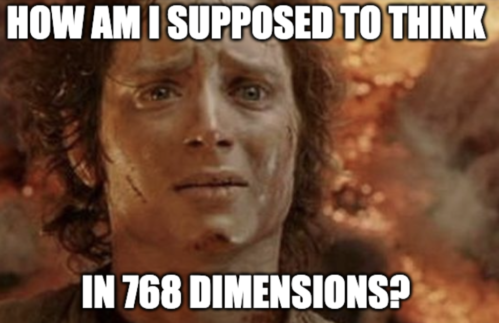
I still struggle with the basic 4 dimensions of our physical world. When I first heard about 768-dimension embeddings, I feared my brain would escape from my ear. If you can relate, if you want to truly master the tricky subject of NLP encoding, this article is for you.

This is a deep dive: over 8,000 words long. Don’t be afraid to bookmark this article and read it in pieces. There is a lot to cover. We will start with basic One-Hot encoding, move on to word2vec word and sentence embeddings, build our own custom embeddings using R, and finally, work with the cutting-edge BERT model and its contextual embeddings.

Like Frodo on the way to Mordor, we have a long and challenging journey before us. Let’s get started.

Our Experiment

The “Lord of the Rings” and “Star Wars” are two iconic franchises that need no introduction. Every day thousands of passionate fans discuss these fictional worlds and characters online. For example:

The above comment doesn’t specifically mention “Lord of the Rings”, but we humans can easily infer which franchise the author is talking about. Another example:

Again, no specific mention of “Star Wars”, but we humans know what’s up. We can easily classify these comments. And in this experiment, we are going to train a machine to do the same thing.

Can different encoding methods help the machine gain better insights into the text? Do some methods result in better predictions than others? How do these different encoding methods compare, all else being equal?

Meet the Model

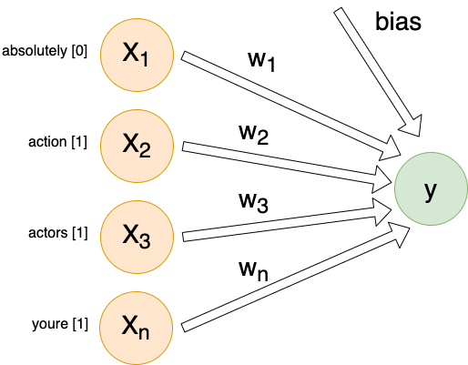
Our classifier is based on the StepByStep class by Daniel Voigt Godoy. It is an extremely simple model:

                    
#define our model
model = nn.Sequential(
    nn.Linear(X, 1) 
)
loss_fn = nn.BCEWithLogitsLoss()
optimizer = optim.Adam(model.parameters(), lr=0.01)

# train it
our_model = StepByStep(model, loss_fn, optimizer)
our_model.set_loaders(train_loader, val_loader)
our_model.train(100)


			

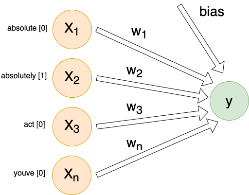
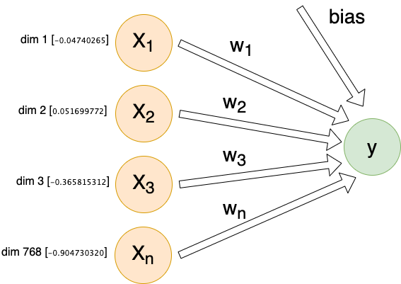
For each individual comment, we will send X inputs (features) into a dense linear layer with a single output. The exact number of inputs will differ depending on encoding method, but they will all follow this same architecture:

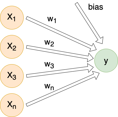
Each input (Xn) is connected to our output by its own weight (Wn). These weights, plus a special bias weight, are the trainable parameters of the model. We begin with random values. With each iteration these parameters (weights) are modified slightly.

This is what is happening behind-the-scenes when we say a model is training and learning. Mathematically speaking, we simply adjust each weight by the partial derivative of our loss function with respect to the given weight, multiplied by our learning rate (η).

Our model uses the Adam optimizer which adjusts our learning rate (η) as it trains. We will use the initial learning rate 0.01. In general practice, that learning rate is really big; we would normally use something closer to 0.0003.

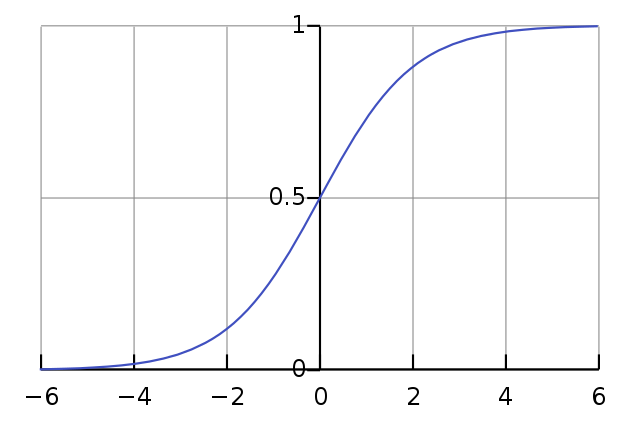
That just leaves our loss function, the heart of any neural network. Since this is a binary classification task, we will use log loss. In general terms, this loss function measures the probability of belonging to the positive class . In our specific case we use BCEWithLogitsLoss which returns logits that must be passed through a sigmoid function to “squish” them back into these probabilities.

For any comments with a probability > 50%, we will classify them as positive. Here we treat “Lord of the Rings” as our positive class, but that is an arbitrary choice. The math works the same either way.

Same model, same data, different encoding methods. Here we go.

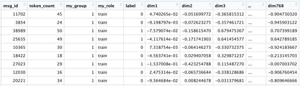
Our Data

On Reddit we find the /r/StarWars and /r/lotr subreddits. We wrote a simple reddit scraper using praw (google colab) to pull comments from each. We pulled about 50,000 comments total, from the “hottest” content around March 1, 2022.

A significant number of these comments were extremely short. They did not contain any useful information. Neither a human nor machine could tell you which subreddit they came from. We randomly selected 10,000 of these 50,000 total comments, each containing at least 13 words (not counting stop words e.g. “the”, “is”, “a”, etc.).

Exactly half of these comments came from /r/StarWars, and the other half from /r/lotr. This allows us to avoid the notorious imbalanced classes issue. If we used a coin flip to guess, or always picked the same franchise, we would expect to be right 50% of the time.

We used this R script to label and organize the data and break it into 5 equally sized 50/50 groups so we could put this data on github.

When training and testing models, we always want to remain mindful of data leakage. We cannot allow any information from outside the training dataset to “leak” into the model. To that end, we will use groups 1, 2 and 3 as our training data (60%), use group 4 as our validation data (20%), and leave group 5 as our testing data (20%).

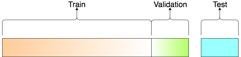
This also helps keep everything as apples-to-apples as possible. Each method will be encoded, trained, validated and tested using the exact same samples.

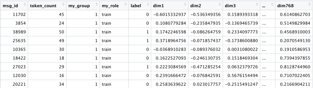
At this point our data looks like this:

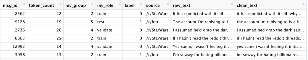
We keep the original raw_text exactly as written, plus a clean_text version, converted to lowercase, with all punctuation and other special characters removed.

Now how do we turn this data into input for our model?

One-Hot Encoding

We will begin with One-Hot encoded inputs. This will allow us to gain some insight into what our model is doing, and define some metrics for our model’s performance. This will also allow us to clearly illustrate the difference between tokenization and encoding.

Tokenizing with Unigrams

Tokenization is the process of turning a full text string into smaller chunks we call tokens. There are many different ways we might tokenize our text. We could use bigrams (“luke skywalker”) or trigrams (“gandalf the grey”), or tokenize parts of a word, or even individual characters. Our options seem infinite.

Here we will tokenize into unigrams, using the tidytext package in R. To avoid data leakage we will use only our training data here.

                    
############################################
# load dependencies
library(tidyverse)
library(tidytext)

############################################################
# load our TRAINING data from github (groups 1, 2, 3)
comments <- read.csv("https://raw.githubusercontent.com/DataJenius/NLPEncodingExperiment/main/data/comments/selected/selected_reddit_comments_group1.csv") %>%
  rbind(read.csv("https://raw.githubusercontent.com/DataJenius/NLPEncodingExperiment/main/data/comments/selected/selected_reddit_comments_group2.csv")) %>%
  rbind(read.csv("https://raw.githubusercontent.com/DataJenius/NLPEncodingExperiment/main/data/comments/selected/selected_reddit_comments_group3.csv"))



			

We will tokenize on clean_text and also filter out any tokens that are stop words (common words such as “the” and “is” and “a”).

                    
############################################################
# define our stopwords and make unigrams from clean_text
words_to_ignore <- stop_words$word
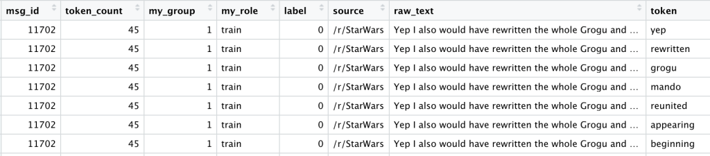
unigrams <- comments %>%
  unnest_tokens(token, clean_text) %>%
  filter(!(token %in% words_to_ignore))


			

Even after filtering, we are left with a very long dataframe, with one row for each occurrence of each token:

Which of these tokens do we care about? How many documents (comments) does each token appear in?

                    
################################################################
# find most important tokens according to document frequency
tokens_by_df <- unigrams %>%
  group_by(token) %>%
  summarise(total_df=length(unique(msg_id))) %>%
  arrange(desc(total_df))


			

Here is a list of the top 20 tokens by document frequency (df):

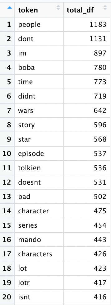
Some of our most frequent tokens (e.g. “story”, “tolkien”, “episode”) seem to offer insight into these two groups. Let’s visualize this:

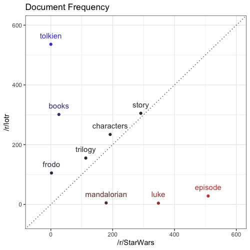
We see that some tokens (e.g. “trilogy”, “characters”, “story”) are used roughly the same by both franchises. Some tokens (e.g. “frodo”, “books”, “tolkien”) are used more often in /r/lotr comments, and others (e.g. “mandalorian”, “luke”, “episode”) are used more often in /r/StarWars comments.

But how do we get this information to our classification model?

Binary Encoding

One-Hot encoding is simple. If a comment includes a given token, we will mark that with a 1. If a comment does not include a given token, we will mark that with a 0. The only tricky part is deciding how many tokens to include. How much dimensionality do we want?

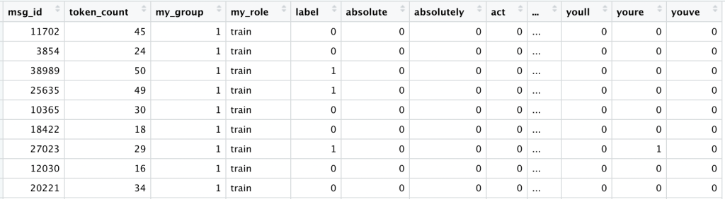
We begin with our top 300 tokens according to the document frequency of the training data. We then use that vocabulary to encode all 10,000 comments. At this point our data looks like this:

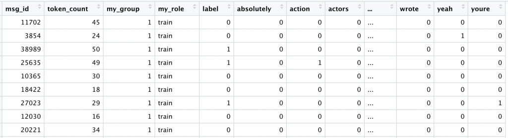
We have added a column for each of our top 300 tokens (starting with “absolutely”, “action”, “actors” and ending with “youre”). For each comment, if it includes a given token we see a 1, otherwise a 0. We can see this One-Hot encoding results in a sparse matrix; most of what it contains are 0’s.

You can find the R script used to one-hot encode the data, and the data itself on github. We started with a raw text string, tokenized it into clean tokens, and encoded these tokens into actual numbers (0 or 1) that can be passed into a neural network as input.

Limitations of One-Hot Encoding

Consider the following made up comments:

As humans we can see these two examples have opposite meanings. Sadly, our One-Hot encodings do not show any difference:

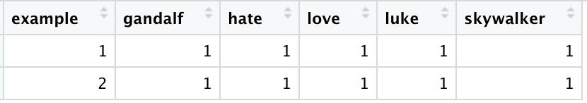
The order of tokens is ignored. Furthermore, only tokens that appear in our pre-defined vocabulary will appear here. Stop words like “I”, “the”, “but”, and less common tokens like “Grey”, simply disappear. We find 38 of these 10,000 comments are One-Hot encoded with all 0’s; they don’t contain any of the top 300 tokens.

Another issue: we only match exact tokens. For the sake of this encoding, “love” and “loved” are two entirely different things, even though, as humans, we understand they are just different forms of the same word. We also ignore how often these tokens are used.

How will our model do given these limitations?

One-Hot (300)

To train and use the model we turn back to python (google colab).

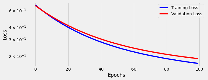
We will pass the model 300 inputs, 0’s or 1’s, for each of our top 300 tokens. This results in 301 total trainable parameters (including the bias parameter which is independent of our inputs).

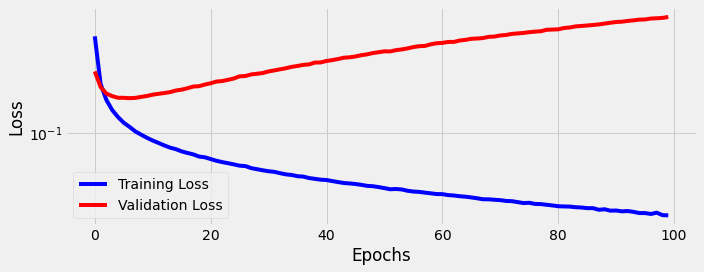
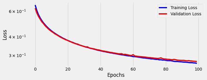
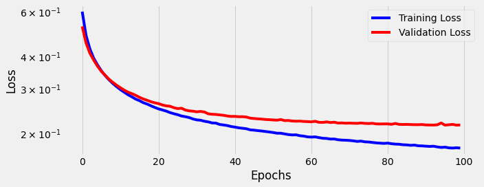
We train for 100 epochs using our training and validation data:

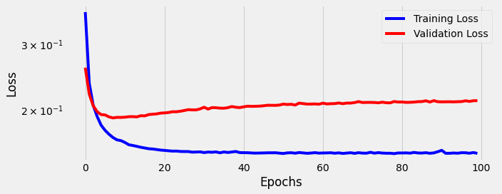
We see the model struggles to learn. As we proceed through 100 epochs the model overfits on the training data; the gap between training loss and validation loss becomes wide, and stays wide.

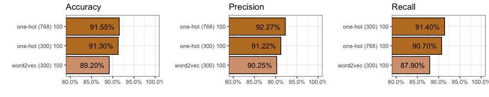
How well does the model do given One-Hot (300) encoding on data it has never seen before (our testing data, group 5)?

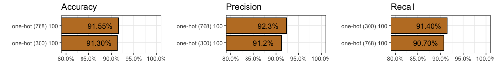
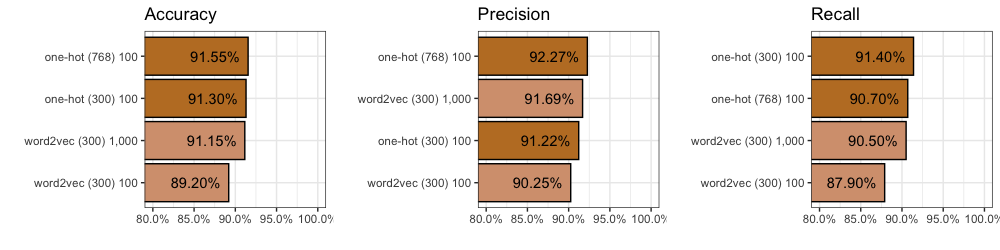
In terms of accuracy we got 91.3%. This means the model correctly classified 1,826 out of 2,000 comments. Not bad.

In terms of precision we got 91.2%. This means that of all the comments our model thought were from “Lord of the Rings”, 91.2% of them were actually from “Lord of the Rings”. It also means 8.8% were really from “Star Wars”.

In terms of recall we got 91.4%. This means that of the 1,000 “Lord of the Rings” comments in our training data (exactly half there are), our model found 914 of them.

You can find all 2,000 individual predictions on github.

One-Hot (768)

Can we make the model perform better by including more tokens? What if we use the top 768 tokens instead?

The data looks pretty much the same, except now we have another 468 columns of 0’s and 1’s. You can find the full data here on github. And you can train and test the model with python (google colab).

The only change to the model is more inputs. Now we have 769 total trainable parameters. We train for the same 100 epochs:

We see the model struggles to learn even more than before. The gap between training loss and validation loss gets wider as we train the model longer and longer.

We find accuracy improves (+0.35%) to 91.55%. We also find precision improves (+1.1%) to 92.3%, but recall decreases (0.7%) to 90.7%. You can find all 2,000 individual predictions on github if you’d like to take a closer look.

Obviously we can keep throwing more and more tokens at our model, but the law of diminishing returns is against us. Is there a better way to encode the information this text contains?

word2vec

Our approach to NLP encoding took a radical leap forward with the 2013 paper Efficient Estimation of Word Representations in Vector Space. Instead of representing each token with a simple 0 or 1, word2vec proposed representing each token as a vector instead.

We can use cosine similarity to compare how similar any two equal-length vectors are to each other:

This allows us find the tokens that are most similar to our given token (“king” in this example):

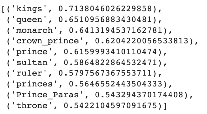
This also allows us to do the following:

Behind-the-scenes this is just vector addition and subtraction. We create a new vector:

We can then use cosine similarity to find which token in our existing vocabulary is most similar to this new hybrid vector:

These word2vec vectors are clearly more informative and flexible than our old One-Hot encoding. Can we use them to improve the performance of our model?

word2vec Tokenization

The original word2vec was trained on roughly 100 billion words from a collection of articles curated by Google News. It contains a vocabulary of 3 million unique tokens. We will tokenize on the same examples from above to see how it compares:

We find that word2vec’s vocabulary includes unigrams like our One-Hot encoding, but also and parts of words:

We see that word2vec’s vocabulary does not include punctuation; both the comma and period have been replaced with [UNK], which represents unknown tokens. We also see word2vec’s vocabulary does not include the name “Gandalf” and instead tokenizes it using two word fragments (“ganda” + “##l” + “##f”). These word fragment tokens allow word2vec to cover a much greater variety in language.

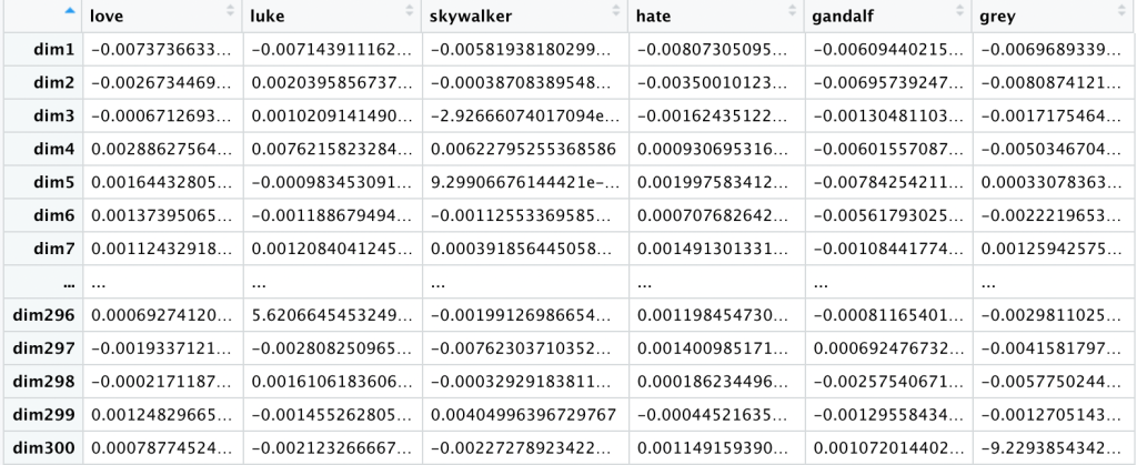
word2vec Word Embeddings

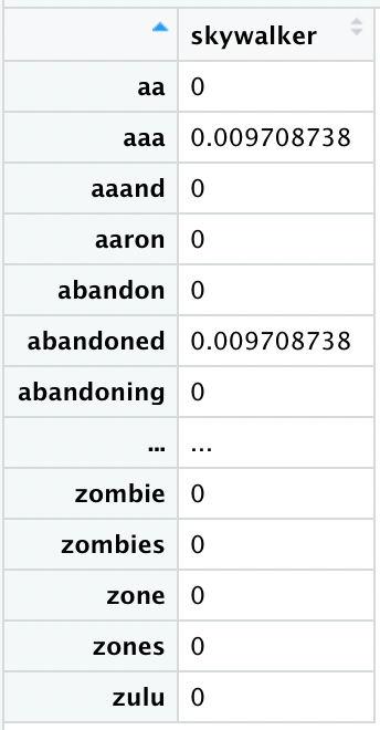
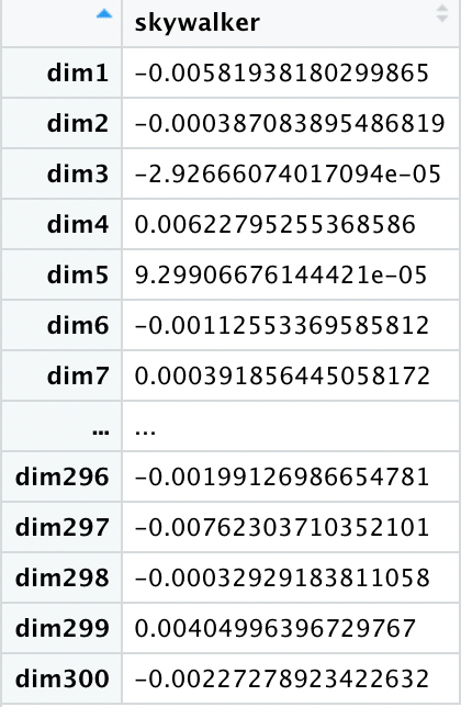
For each token in word2vec’s vocabulary, we have a 300-dimension word embedding, a vector with a series of 300 numbers.

For special tokens (e.g. [UNK]) we simply use a vector of 300 zeros:

Once we have tokenized our text, we simply grab the corresponding pre-trained word2vec word embedding for each of them. This includes our word fragment tokens like “##l” and “##f”.

word2vec Sentence Embeddings

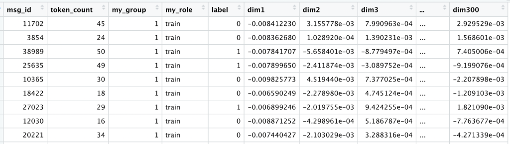
We have 10,000 comments, each with a variable number of tokens, each of which is associated to a 300-dimension word embedding. How do we turn this mess into useable input for our model?

The first thing we will do is deal with the fact that our comments have variable numbers of tokens. We will set a max token length of 500, and truncate any comments that are longer than that. For comments shorter than 500 tokens, we will pad them with vectors of 300 zeros.

For example:

This is tokenized by word2vec like so:

And encoded like so:

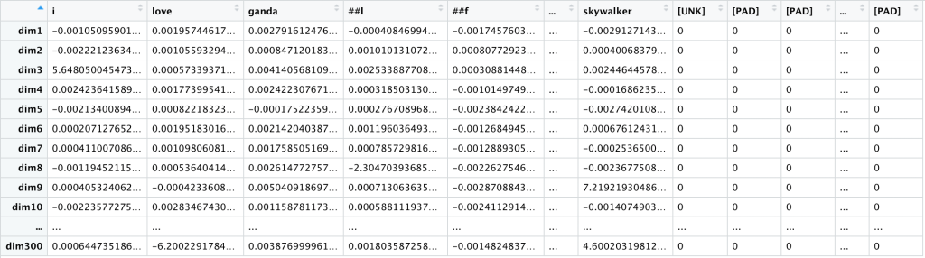
We now have exactly 500 columns left-to-right, one for each token in this comment, plus as many [PAD] tokens as needed. We also have exactly 300 rows, one for each of our 300 dimensions.

There are many different ways we might combine these token-based word embeddings into full sentence (comment) embeddings. One simple method is to take the average of each dimension, the row-wise mean of the above dataframe. If we take those averages and transpose them (rotate 90°) we get something that resembles our One-Hot encoding from above.

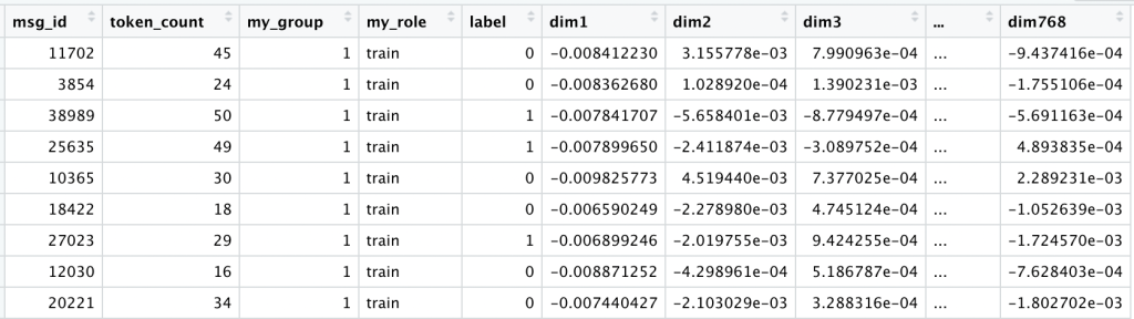
At this point our data for all comments looks like this:

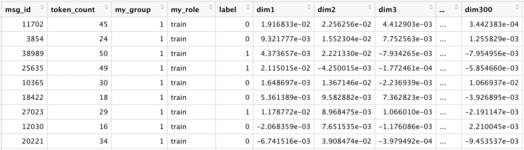
Now we have one row for each comment, plus an additional 300 columns (our features X). However, instead of a simple 0 or 1 for a select vocabulary of tokens, we now have the average of each dimension of our 300-dimension word embeddings. What was once a sparse matrix full of 0’s is now dense with information.

Because these word2vec embeddings are pre-trained, we can encode all of our data at the same time without any fear of data leakage. You can find the full data here on github. And you can extract these embeddings yourself with python (google colab).

Limitations of word2vec

In theory, word2vec offers some advantages over One-Hot. For example, One-Hot ignores how often tokens are used. With word2vec, repeated tokens serve as a sort of weighted average in our sentence embeddings. We also noted that, in terms of One-Hot encoding, the tokens “love” and “loved” are completely different things. Not true of these word2vec embeddings:

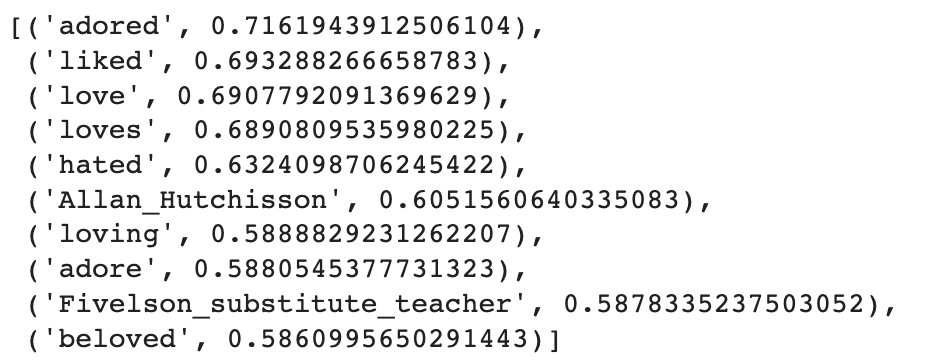
We see that the most similar tokens to “loved” not only include “love” but also “loves”, “loving”, “adore” and other synonyms and antonyms. This also shows how embeddings like these are able to deal with common slang, typos, and other eccentricities of natural language.

However, as with our One-Hot encoding, the order of tokens is still ignored. The “I love/hate Luke Skywalker, but I love/hate Gandalf the Grey.” examples still result in identical encodings. Furthermore, any tokens that do not appear in word2vec’s 3,000,000 token vocabulary will be encoded as zeros and lost.

And the biggest limitation to these word2vec embeddings? They were trained almost 10 years ago, on data not very similar to our Reddit comments. Consider the tokens most similar to “luke”:

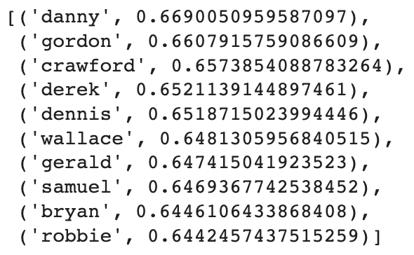
It appears “luke” is associated to other common first names, nothing specific to our Jedi hero. And the tokens most similar to “skywalker”?

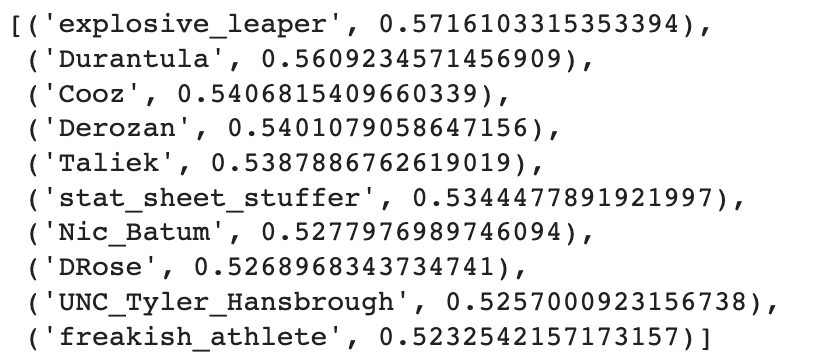
I’m not sure what these tokens have in common. Is this new word2vec encoding truly better than the old One-Hot 0’s and 1’s?

word2vec (300)

To train and use the model we turn back to python (google colab).

We will pass the model 300 inputs, the means of each of our 300 dimensions of word2vec embeddings for each comment. This results in 301 total trainable parameters (including the bias).

We train for 100 epochs using our training and validation data:

We see the model is now learning. The gap between training loss and validation loss is small, and both continue to decrease as the model trains longer and longer.

However, compared to our One-Hot inputs with 300 dimensions, after 100 epochs, we find accuracy decreases (-2.1%) to 89.2%. We also find precision drops (-0.97%) to 90.25%, and recall decreases (-2.8%) to 87.9%. You can find all 2,000 individual predictions on github if you’d like to take a closer look.

We continued training for 1,000 epochs:

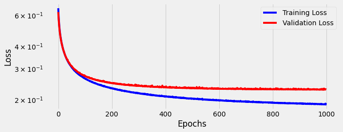
Even after 1,000 epochs we found accuracy failed to beat our One-Hot inputs (-0.15%) with 91.15%. We find an improvement in precision (+0.47%) to 91.69%, but recall decreases (-0.2%) to 90.5%. You can find all 2,000 individual predictions on github.

Does this mean all these fancy vector encodings are a waste of time?

Custom Embeddings

The name “word2vec” usually refers to the pre-trained 300-dimensional word embeddings used above . However, “word2vec” can also refer the actual model used to train these embeddings in the first place. We aren’t stuck with these pre-trained vectors. We can build our own using the word2vec model and our own specific text.

Sure, we could just reuse the word2vec model, but what fun is that? In order to truly dig in and understand these embeddings, we are going to make our own, from scratch, using R.

The Theory

The theory behind word2vec is deceptively simple:

You shall know a word by the company it keeps.

John Rupert Firth

At the heart of any neural network we find a loss function, and word2vec is no exception:

Although this formula appears intimidating at first, it can be reduced to some very simple ideas. (T) is the total number of tokens in our corpus. We loop through each of these tokens (t) one-by-one. At each token we look at a window of size (m) to see which tokens are our neighbors. To use an example, imagine the text:

I think machine learning is super cool.

Let us assume m=2 and t=5 for the sake of this example. This means we have reached the 5th token (“is”):

Our m window of 2 means we look at the two words in front of “is”, and the two words that follow. Note that m=2 is an arbitrary choice, determined by the researcher.

One heuristic is that smaller window sizes (2-15) lead to embeddings where high similarity scores between two embeddings indicates that the words are interchangeable. […] Larger window sizes (15-50, or even more) lead to embeddings where similarity is more indicative of relatedness of the words.

Jay Alammar, The Illustrated Word2vec

Recall this term of our loss function:

Here this simply means:

It all comes down to basic probability. How likely is a context token given a specific target token?

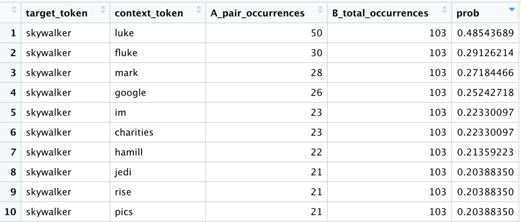
Let us simplify the above math. Let A equal the number of comments in which a target token appears together with a context token. Let B equal the number of comments in which the target token appears overall. Our probability is now a simple A/B.

Let us illustrate with an example:

The token “skywalker” appears in 103 of our training comments. The tokens “skywalker” and “luke” appear together in 50 of our training comments. Therefore the probability of seeing the context token “luke” given the target token “skywalker” is roughly 50%.

Embeddings from Scratch

We can create custom embeddings with less than 200 lines of R code. Actually, we could do it more efficiently than that, but this code is intentionally verbose for the sake of a teaching example.

Because we are considering the entire comment regardless of length, our m window is now variable- the length of each individual comment. This results in the largest possible window, the largest possible m, and yields embeddings where similarity is more indicative of the relatedness of the words.

To avoid data leakage, we will build these custom embeddings based on our training data only:

                    
############################################################
# load our TRAINING data from github (groups 1, 2, 3)
comments <- read.csv("https://raw.githubusercontent.com/DataJenius/NLPEncodingExperiment/main/data/comments/selected/selected_reddit_comments_group1.csv") %>%
  rbind(read.csv("https://raw.githubusercontent.com/DataJenius/NLPEncodingExperiment/main/data/comments/selected/selected_reddit_comments_group2.csv")) %>%
  rbind(read.csv("https://raw.githubusercontent.com/DataJenius/NLPEncodingExperiment/main/data/comments/selected/selected_reddit_comments_group3.csv"))


			

Again we tokenize into unigrams. B is simply the document frequency from before. We limit our vocabulary to tokens that have appeared in at least 2 comments:

                    
############################################################
# define vocabulary that appears in at least 2 documents
# we have 10,161 unique tokens (our vocabulary)
vocab <- unigrams %>%
  group_by(token) %>%
  summarise(B_total_occurrences=length(unique(msg_id))) %>%
  arrange(desc(B_total_occurrences)) %>%
  filter(B_total_occurrences >= 2) %>%
  rename(target_token=token)



			

We can get A from the pairwise_count function: the number of times each context token appears with a given target token.

                    
############################################################
# define all pairs of our 10,161 vocab words 
vocab.pair <- unigrams %>%
  # only consider tokens in vocab
  filter(token %in% vocab$target_token) %>%
  # find A the occurrences of both tokens
  pairwise_count(token, msg_id, diag=FALSE) %>% # include diagonal (always 100%)
  rename(target_token=item1,
         context_token=item2,
         A_pair_occurrences=n)


			

We join the two together and calculate prob as A/B:

Next we cast this probability into a matrix where each row represents a target token and each column represents a context token. We have 10,161 rows and columns, one for each token in our vocabulary:

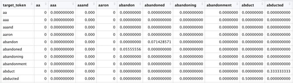
Once again we have a sparse matrix. If we take the row for a single target token and transpose it, what we are left with is a de-facto 10,161-dimension word embedding. Each dimension represents the probability of each of the 10,161 potential context tokens:

There are many different methods of dimensionality reduction we might use, including PCA, t-SNE and SVD, just to name a few. Here we will use IRLBA in order to reduce from 10,161 dimensions down to 300 dimensions, the same number our word2vec embeddings have:

Our sparse matrix has become dense with information, but the trade-off is interpretability. We had 10,161 rows, each corresponding to a specific context token probability. Once reduced to 300, our dimensions no longer refer to a specific token. This makes it very hard to define what a given dimension is capturing in terms a human can understand.

We can, however, understand the essence of this new custom embedding: we have preserved the most important information contained in the above probability matrix.

Custom Sentence Embeddings

How do we use these new custom embeddings to encode our full comments? Our method will be similar to our word2vec sentence embeddings above, with one notable difference.

Instead of padding and truncating our comments to a standard number of tokens, we will simply consider all the tokens in each comment that can be found in our vocabulary. Any tokens not in our vocabulary will be ignored. Any comment without any known tokens will be encoded with 300 zeros instead.

Our custom vocabulary still includes 10,161 different unigrams. Each of these tokens is associated to one of the 300-dimension custom word embeddings we made above.

For example:

This is tokenized based on our custom vocabulary like so:

And encoded like so:

To reduce this into a sentence embedding, once again we will take the average per dimension (the row-wise mean) and transpose it. At this point our data for all comments looks like this:

You can find the full encoded data here on github. And you can encode this data for yourself using this R script.

Limitations of Custom

The order of tokens is still being ignored. The “I love/hate Luke Skywalker, but I love/hate Gandalf the Grey.” examples will still result in identical encodings. Furthermore, any tokens that do not appear in our custom 10,161 unigram vocabulary will be ignored.

However, these custom embeddings seem to capture the essence of our comments far better than the pre-trained word2vec embeddings. Consider the most similar tokens for “luke” and “gandalf”:

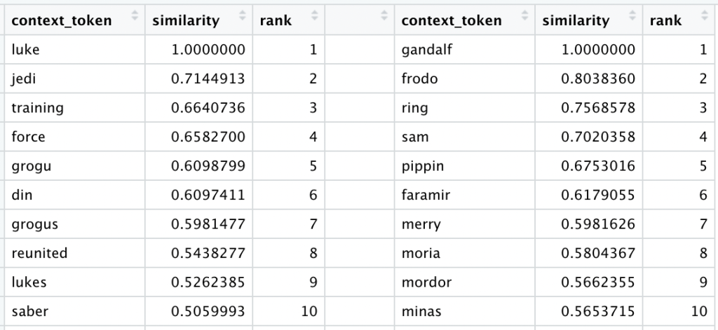
These similar tokens make a lot more sense now. Do we finally have an encoding that can beat the old One-Hot 0’s and 1’s?

Custom (300)

To train and use the model we turn back to python (google colab).

We will pass the model 300 inputs, the means of each of our 300 dimensions of custom embeddings for each comment. This results in 301 total trainable parameters (including the bias).

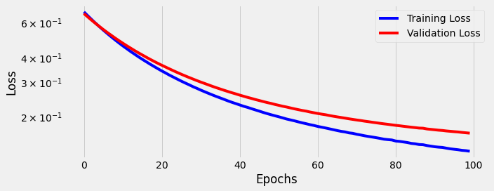
We train for 100 epochs using our training and validation data:

We see the model is learning. Both training loss and validation loss continue to decrease as the model trains longer and longer.

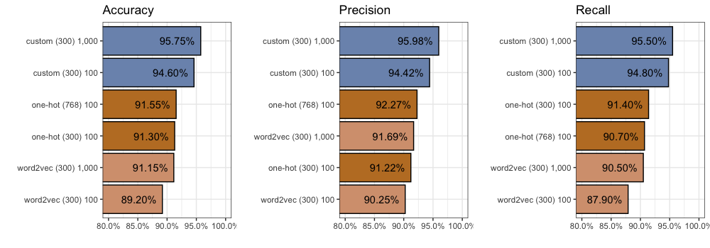
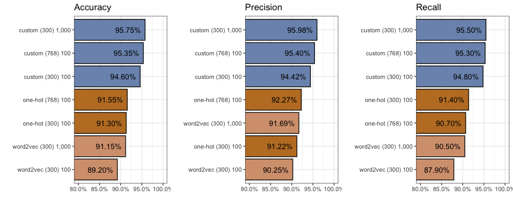
We find considerable improvement compared to our One-Hot inputs with 300 dimensions. After 100 epochs, accuracy increases (+3.3%) to 94.6%, precision increases (+3.2%) to 94.42%, and recall increases (+3.4%) to 94.8%.

You can find all 2,000 individual predictions on github.

We continued training for 1,000 epochs:

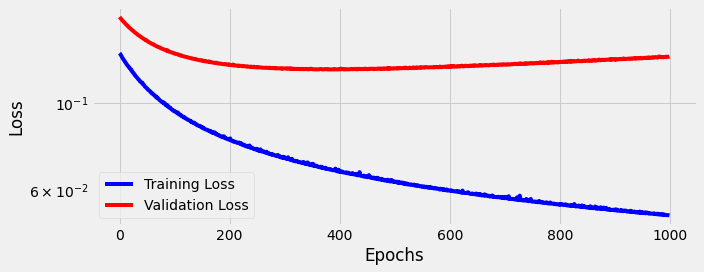
This training/validation loss curve isn’t as pretty now. After around 400 epochs it struggles to learn further, and starts to “unlearn” slightly as we approach 1,000 epochs.

Despite this, we see another jump in performance. Accuracy increases another +1.15% to 95.75%, while precision increases another +1.56% to 95.98%, and recall increases another +0.7% to 95.5%. Again you can find all 2,000 individual predictions on github.

It looks like our custom embeddings are pretty powerful.

Can we do better?

Custom (768)

What happens if we increase our custom embeddings to 768 dimensions?

The data looks pretty much the same, except now we have another 468 columns of dense custom embedding inputs. You can find the full data here on github. And you can train and test the model with python (google colab).

The only change to the model is more inputs. Now we have 769 total trainable parameters. We train for the same 100 epochs:

Once again we see the model is learning; training and validation loss decrease as the model trains longer and longer.

Given these additional dimensions, we find more improvement. Compared to our custom embeddings with 300 dimensions, after 100 epochs each, accuracy increases (+0.75%) to 95.35%, precision increases (+0.98%) to 95.4%, and recall increases (+0.5%) to 94.8%. You can find all 2,000 individual predictions on github.

We continued training for 1,000 epochs:

Again the model starts to “unlearn” around the 400th epoch. Performance remains largely unchanged. We are unable to beat 300 dimensions with 768 dimensions after 1,000 epochs.

We could keep adding dimensions and training epochs, but once again we are facing the law of diminishing returns. If we want to improve performance further, we will need a different strategy.

BERT

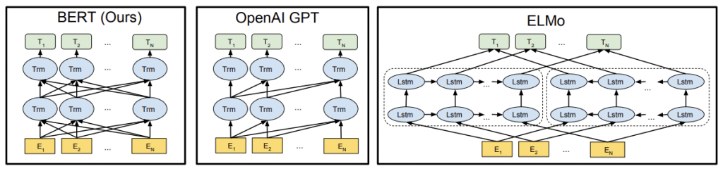
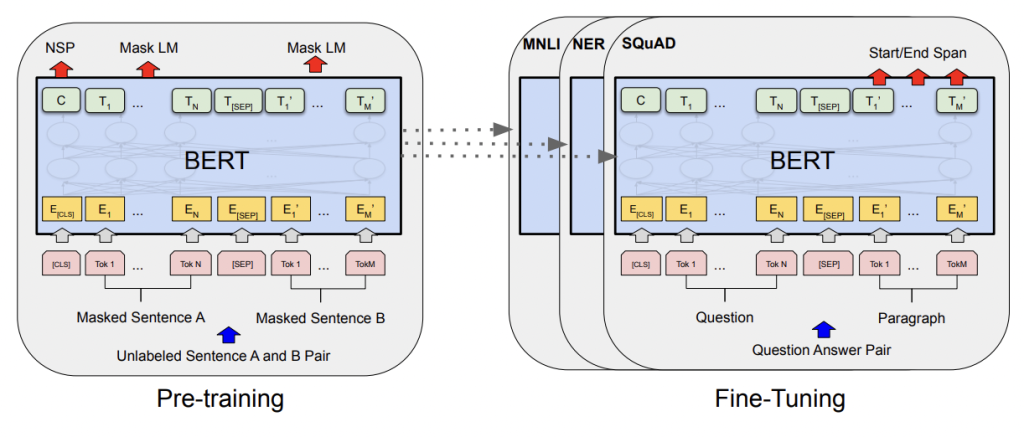
BERT (Bidirectional Encoder Representations from Transformers) combined the unsupervised pre-training of a transformer (OpenAI GPT) with embeddings that consider the bidirectional context of tokens (eLMo). When released in 2019, BERT was capable of producing state-of-the-art results for 11 different NLP tasks. Here we are concerned with only one of those tasks: classification.

BERT Masking

One of the things BERT does is use masks in order to predict a token given the context of surrounding tokens. For example:

How does this differ from word2vec?

Until now, all of our encoding schemes have ignored the order of our tokens. A word2vec embedding trained with a window of m=9 would include “love”, “hate”, “Luke Skywalker” and “Gandalf the Grey”, but have no additional context beyond that.

By comparison, BERT is bidirectional. In other words, not only does BERT consider the order of tokens, it considers them both left-to-right and right-to-left.

At long last, the “I love/hate Luke Skywalker, but I love/hate Gandalf the Grey.” examples will result in different encodings, based on the specific order of the tokens.

BERT Tokenization

Let’s take a closer look at the BERT tokenizer:

This is tokenized by BERT like so:

The first thing we notice about BERT tokenization is the special [CLS] token added to the start of our comment. This is going to be critical in the next step. We also find [SEP] tokens at the end of our comments. Unlike word2vec, BERT tokenization includes punctuation. Our comma and period remain.

We find that text tokenized by BERT, like word2vec, includes parts of words. However, unlike word2vec, BERT uses the WordPiece algorithm in order to define these subword tokens.

Intuitively, WordPiece is slightly different to BPE in that it evaluates what it loses by merging two symbols to ensure it’s worth it.

HuggingFace Documentation

BERT has a vocabulary of only 30,522 unique tokens, compared to word2vec’s vocabulary of 3 million. Despite this, we find that the BERT tokenizer with WordPiece is more versatile. It can handle pretty much whatever you throw at it:

As before, when it encounters something unknown (in this case our 😜 emoji) you will see the special [UNK] token in its place.

These tokens look good. But how do we get our embeddings?

BERT Sentence Embeddings

For our word2vec and custom sentence embeddings above, our process was roughly the same:

1. Tokenize our text and extract all known tokens
2. Encode each known token with the corresponding word embedding
3. Use the dimension-wise average as the sentence embedding

BERT, like word2vec above, uses truncation and padding to turn comments (each with a variable number of tokens) into a standard size tensor. However, this is where the similarities end.

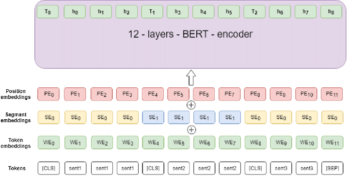
BERT uses 12 transformer layers and 12 self-attention heads in order to focus on different sections of each text (reading both left-to-right and right-to-left). The resulting embeddings are based (in part) on the order of tokens, and the exact position of the token in question. This is how BERT is able to train and learn 768-dimension contextual embeddings for each token.

This includes the special [CLS] token mentioned above.

We will use this special [CLS] embedding, rather than a dimensional average, for our downstream task (predicting which franchise a comment belongs to). As we see below, this is exactly what the BertForSequenceClassification model does:

                    
BertForSequenceClassification(
  (bert): BertModel(
    (embeddings): BertEmbeddings(
      (word_embeddings): Embedding(30522, 768, padding_idx=0)
      (position_embeddings): Embedding(512, 768)
      (token_type_embeddings): Embedding(2, 768)
      (LayerNorm): LayerNorm((768,), eps=1e-12, elementwise_affine=True)
      (dropout): Dropout(p=0.1, inplace=False)
    )
    (encoder): BertEncoder(
    	** 12 layers of self-attention goodness **
    )
    (pooler): BertPooler(
      (dense): Linear(in_features=768, out_features=768, bias=True)
      (activation): Tanh()
    )
  )
  (dropout): Dropout(p=0.1, inplace=False)
  (classifier): Linear(in_features=768, out_features=2, bias=True)
)


			

We used this python script (google colab) to extract the output of the BertPooler above. Note that we used the pre-trained (pt) “bert-based-uncased” model to get these. Like the our word2vec input above, this BERTpt input is not based on any of our own comment data. These embeddings are based on what BERT saw back in 2019 when it was originally trained.

                    
bert_model = TFBertModel.from_pretrained(
    'bert-base-uncased', 
    trainable=False, 
    num_labels=2)


			

At this point our data is almost identical to custom (768), just with different values for each dimension. It looks like this:

You can find the full encoded data here on github.

BERTpt (768)

To train and use the model we turn back to python (google colab).

We will pass the model 768 inputs, the pre-trained BERT [CLS] embeddings for each comment. This results in 769 total trainable parameters (including the bias).

Because the values of these BERTpt embeddings are significantly larger that the others, we reduced our initial learning rate (η) to 0.0003 to compensate. Then we train for 100 epochs using our training and validation data:

We see that our same simple classification model is able to learn from these fancy BERT embeddings too. Both training loss and validation loss decrease as the model trains.

How well do these new BERTpt embeddings do as input?

In a word: disappointing. The BERTpt input fails to outperform the one-hot or word2vec inputs. Custom still reigns supreme. You can find all 2,000 individual predictions on github.

Does this mean using BERT is a waste of our time? Not so fast.

Fine-tuning BERT

As mentioned above, BERT uses 12 transformers and 12 self-attention heads in order to generate these embeddings. However, the above pre-trained encoding didn’t take full advantage of that.

The excellent Illustrated BERT, ELMo, and co. (How NLP Cracked Transfer Learning) by Jay Alammar can help provide readers with some additional context. For our purposes the key point is this: we can fine-tune BERT.

Unlike prior attempts at transfer learning, BERT allows us to fine-tune using all 109,483,778 of its trainable parameters. This results in the best possible representations of our specific text.

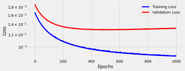
Once again we remain mindful of data leakage. We restrict this tuning to our training and validation data only, and keep our test data unseen. We used this python script (google colab) to fine-tune BERT for a single epoch. We then extracted these fine-tuned (BERTft) embeddings for all 10,000 comments for use in our own model.

While extracting these embeddings you will encounter the biggest limitation of BERT. Compared to our simple model, which trains and predicts in under five minutes, BERT can feel painfully slow. It took roughly 4 hours to complete a single epoch of fine-tuning. Why so long? Because we are fine-tuning 109,483,778 trainable parameters. That’s a lot of math.

Our end result is almost identical to custom (768) and BERTpt (768). All that changes is the specific values for each dimension.

It looks like this:

You can find the full encoded data here on github.

BERTft (768)

To train and use the model we turn back to python (google colab).

We will pass the model 768 inputs, the fine-tuned BERT [CLS] embeddings for each comment. This results in 769 total trainable parameters (including the bias).

We reduce our initial learning rate (η) to 0.00001 and train for 100 epochs using our training and validation data:

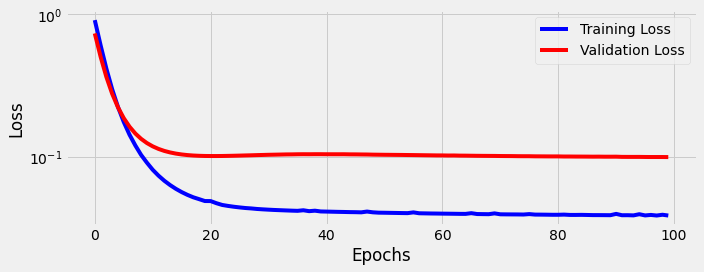
Both training loss and validation loss decrease as the model trains, but learning seems to level off after around 18 epochs.

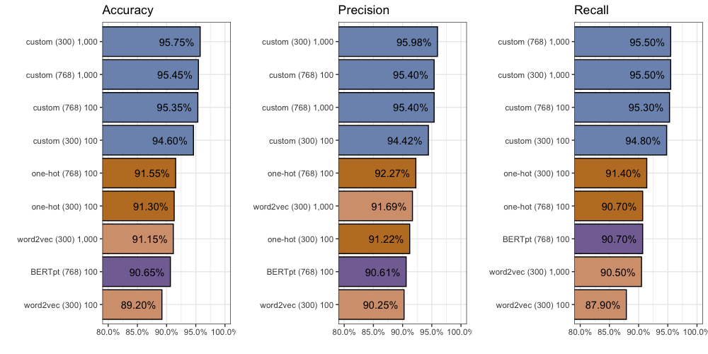
Now the million dollar question: how do fine-tuned BERT embeddings compare to our best custom embeddings? We find accuracy improves (+0.65%) to 96.4%, precision improves (+0.61%) to 96.59%, and recall increases (+0.7%) to 96.2%.

You can find all 2,000 individual predictions on github if you’d like to take a closer look.

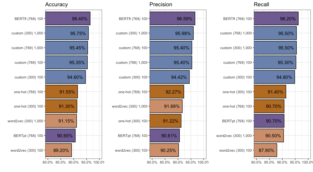
Eat your heart out, custom. It looks like BERT is the new sheriff in town.

Comparing our Methods

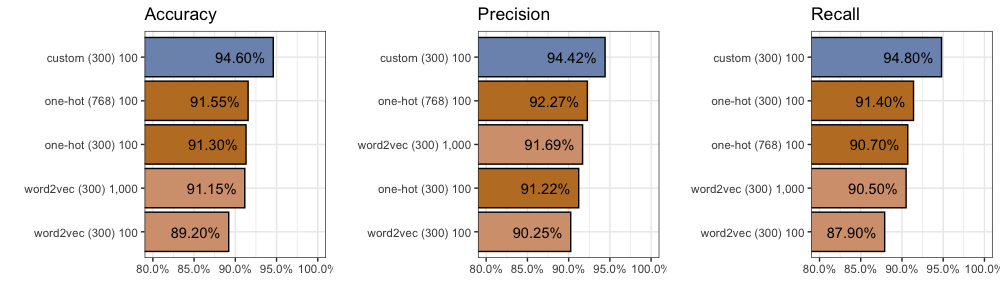
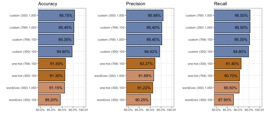
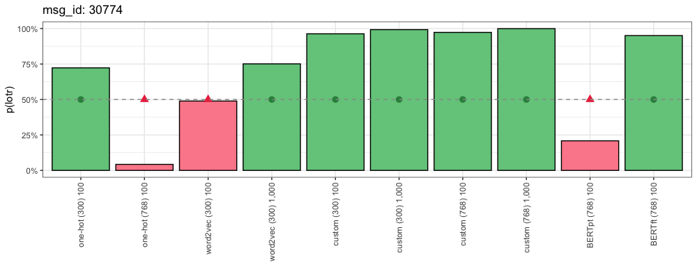
Here is a quick recap of the 10 different methods we have tried:

Beyond these statistics, we can gain some more intuition towards these different input methods by looking at some specific examples.

Easy Examples

Recall that our model predictions include the probability of belonging to the positive class (“Lord of the Rings”). This means we can look beyond accuracy, precision and recall, and see how confident the model was for each answer.

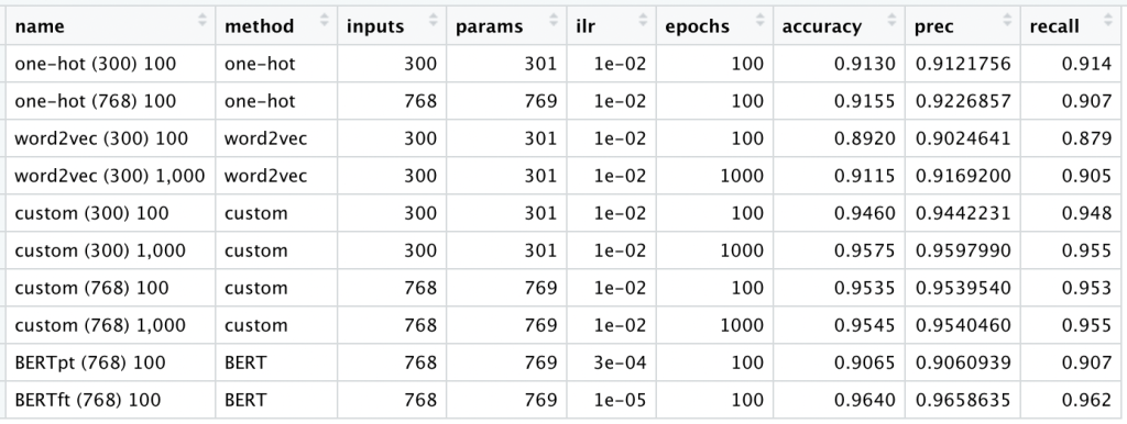
Consider this comment (from “Star Wars”):

This is how each method responded:

Our decision boundary is 50% (the dotted line). Everything over that line is classified as “Lord of the Rings”. Because this example comes from “Star Wars”, here we want all of these probabilities to be as low as possible. The closer a method is to 0%, the more confident it is that this is a “Star Wars” comment.

We can see that although our word2vec methods got this one right, they were the least right of the 10 methods tested. Compare to One-Hot and BERT which are much closer to 0%.

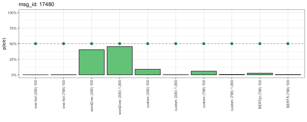
Consider this comment (from “Lord of the Rings”):

This is how each method responded:

Because this comment is from our positive class (“Lord of the Rings”) here we want to see all of these probabilities as high as possible. The closer a method is to 100%, the more confident it is that this is a “Lord of the Rings” comment.

These comments are both rich with franchise-specific terms like “Jedi”, “Ben Kenobi”, “Luke Skywalker”, “Hobbit” and even “The Lord of the Rings”. We can understand why all methods got these right- these were some easy ones.

Not As Easy Examples

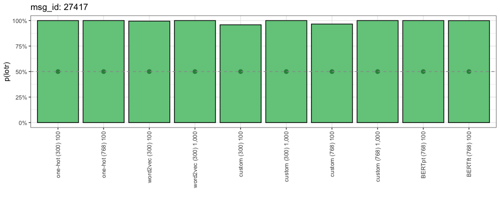
Consider this comment (from “Lord of the Rings”):

This is how each method responded:

We humans recognize “Two Towers” as the title of one of the “Lord of the Rings” books. Why did our One-Hot encodings struggle here? Because the critical token “towers” does not appear in the vocabularies of One-Hot (300) or One-Hot (768). And the pre-trained word2vec and BERT embeddings don’t recognize the significance of “Two Towers” here.

Compare to our custom (300) embeddings:

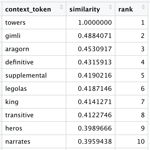
Not only does our custom vocabulary include “towers”, it associates that token to “gimli”, “aragorn” and “legolas”. Presumably our fine-tuned BERT embeddings were able to find a similar pattern, and come to a similar conclusion.

Our next comment (from “Star Wars”) dares to discuss the important issues: Does “Jabba the Hutt” reproduce asexually?

This is how each method responded:

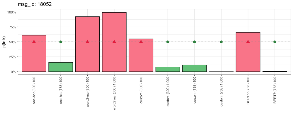
Similar to above, the critical token “hutts” does not appear in the vocabularies of One-Hot (300) or One-Hot (768). Likewise, the pre-trained word2vec and BERT embeddings don’t recognize this as a character from “Star Wars”. Even our custom (300) and custom (768) embeddings disagree here.

Let’s take a closer look at the most similar tokens to “hutts” according to both custom (300) and custom (768):

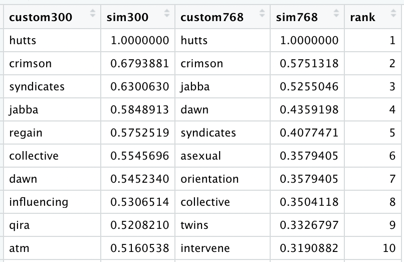
Both embeddings associate back to “jabba”, but only custom (768) contains enough dimensionality to also associate with “asexual” and “orientation”. Note that both custom embeddings (300 and 768) include the same 10,161 token vocabulary.

It takes custom (300) 1,000 epochs to get it right. With the added dimensionality, custom (768) figures it out after only 100.

Where BERT Prevails

Consider this comment (from “Star Wars”):

This is how each method responded:

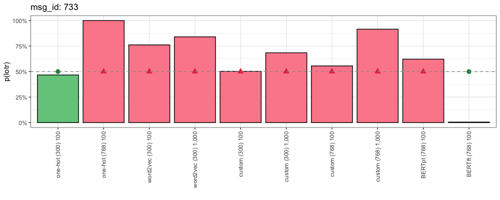
This comment uses slang (“Mando”, “BoBF”) to refer to the shows “The Mandalorian” and “The Book of Boba Fett”. The token “mando” appears in all of our One-Hot and custom vocabularies. “bobf” appears in our custom and One-Hot (768) vocabularies. Despite this, only our fine-tuned BERT embeddings resulted in a confident right answer.

Consider this comment (from “Lord of the Rings”):

This is how each method responded:

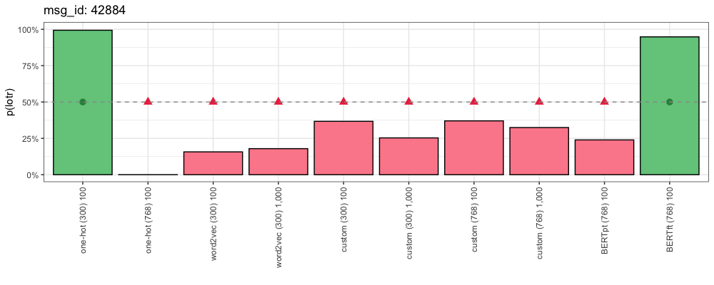
Here is an interesting case where only our most simple encoding (One-Hot with top 300 tokens) and our most complicated encoding (fine-tuned BERT) got the right answer. And they are both pretty confident about it. What is going on here?

Out of our 298 training examples that included the token “book”, 70.5% of them came from “Lord of the Rings”.

Our One-Hot (300) encoding focuses on “book” because (a) it only looks for 300 tokens in the first place, and (b) this is the most relevant token in this example.

Our fine-tuned BERT encoding also focuses on the token “book”, despite having more than 100 million additional trainable parameters. This is the power of self-attention, and a good example of how BERT learns which parts of a text are the most relevant.

Given the length of this comment, our other encoding methods get overwhelmed with too much information. Once we look for 768 One-Hot encoded tokens, or take the dimension-wise averages of all the tokens this comment contains, our encodings lose their focus on “book”, and confuse the model.

Sentence Similarity

When looking at our word embeddings above, we used cosine similarity to rank how close tokens are to each other.

Can we use this same function to see how similar our sentence embeddings are to each other? Yes we can.

Custom Similarity

Consider the following comment (from “Lord of the Rings”):

If we compare the cosine similarities of our custom (768) sentence embeddings, we find this is the most similar comment:

For the sake of comparison, here is another comment which also contains the name “Gandalf”, but has a much lower similarity score:

This comment mentions “Gandalf”, but not his true power. We can see how this is less similar to the original comment.

BERT Contextual Embeddings

Consider the following examples:

He is over 7 feet tall.

Did you measure in feet or meters?

In these examples, “feet” refers to a measurement of 12 inches.

After playing basketball my feet hurt.

Her feet are in need of a pedicure.

In these examples, “feet” refers to the things attached to the bottom of your legs. This is a common phenomenon in natural language: the same words can have different meanings, depending on their context.

Let us compare to this example:

My feet are too big for these shoes.

When we convert these into pre-trained BERT embeddings and compare cosine similarity, we see something amazing:

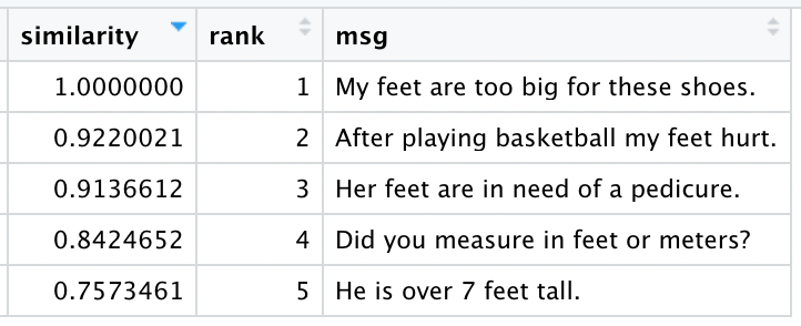
The BERT embeddings for “feet” (with toes) are more similar than the embeddings for “feet” (12 inches). The 12 transformers and self-attention heads of BERT are powerful enough to produce more informative embeddings.

Consider the following:

He failed his driver test because he can’t parallel park.

Where do you park this big truck?

In these examples, “park” refers to the act of putting a vehicle to rest.

Turing Park is full of trees and flowers.

We should walk over to the park today.

In these examples, “park” refers to a place you might want to go.

Let us compare to this example:

I took the kids to the park so they could play.

Again we convert these into pre-trained BERT embeddings and compare cosine similarity, and again we see something amazing:

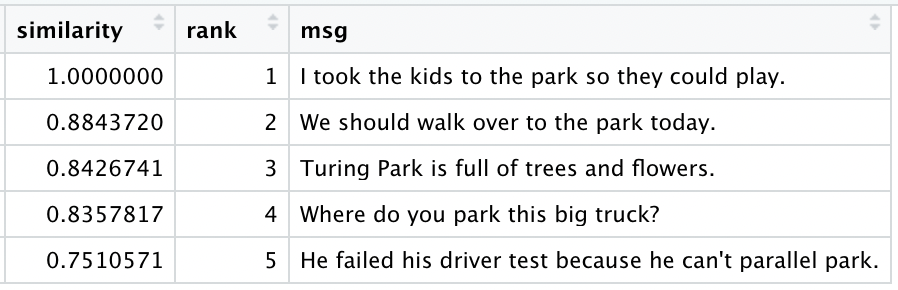
The BERT embeddings for “park” (noun) are more similar than the embeddings for “park” (verb). Once again BERT demonstrates the power of context in understanding natural language.

Conclusion

Back in the ancient times, before 2013, we usually encoded basic unigram tokens using simple 1’s and 0’s in a process called One-Hot encoding. word2vec improved things by expanding these 1’s and 0’s into full vectors (aka word embeddings). BERT improved things further by using transformers and self-attention heads to create full contextual sentence embeddings.

Beyond use in this classification example, these embeddings are powerful. They allow us to do math with words:

These embeddings also allow us to find the meaning of specific tokens, and compare the similarity of full sentences (comments). We can use BERT embeddings for many other tasks too, such as extracting a questions/answers model, or summarizing key points of text. This article has only scratched the surface in regards to BERT’s full capabilities.

When training models, it is often tempting to toss more features at it, train for more epochs, and hope for the best. This article demonstrates the diminishing returns such an approach will yield.

Instead we must think deeply about the information our text contains, and how we can represent that information numerically. As the above experiment proved, how we choose to encode our data can make all the difference.

Want more content like this? Please subscribe and share below:

How can convolutional filters, which are designed to find spatial patterns, work for pattern-finding in sequences of words? This post will discuss how convolutional neural networks can be used to find general patterns in text and perform text classification. The end of this post specifically addresses training a CNN to classify the sentiment (positive or negative) of movie reviews.

Encoding Words

First, how do we represent text and prepare it as input into a neural network? Let’s focus on the case of classifying movie reviews, though the same techniques can be applied to articles, tweets, search queries, and so on. In the case of movie reviews, we have hundreds of text reviews. Each of which is a few, opinionated sentences long; the length varies.

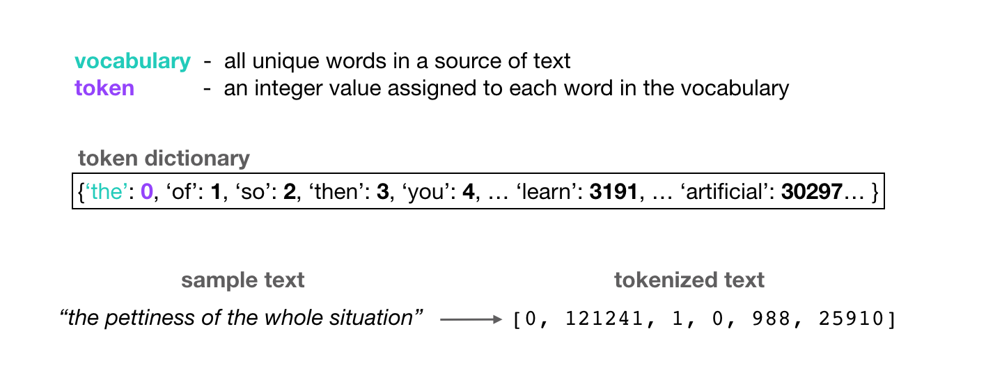
Neural networks can only learn to find patterns in numerical data and so, before we feed a review into a neural network as input, we have to convert each word into a numerical value. This process is often called word encoding or tokenization. A typical encoding process is as follows:

1. For all of the text data—in this case, the movie reviews—we record each of the unique words that appear in that dataset and record these as the vocabulary of our model.
2. We encode each vocabulary word as a unique integer, called a token. Often, these tokens are assigned based on the frequency of occurrence of a word in the dataset. So, the word that appears most frequently throughout the dataset, will have the associated token: 0. For example, if the most common word was “the,” it would have the associated token value of 0. Then the next most common word will be tokenized as 1, and that process continues.

3. In code, this word-token association is represented in a dictionary that maps each unique word to their token, integer value:

   {'the': 0, 'of': 1, 'so': 2, 'then': 3, 'you': 4, … }

   There are often so many words in a given dataset that these tokens will range from the value 0 to 100,000 or so.

4. Finally, after assigning these tokens to individual words, we can then tokenize the entire corpus.

For any document in a dataset, like a single movie review, we treat it as a list of words in a sequence. Then we use the token dictionary to convert this list of words into a list of integer values.

It’s important to note that these token values do not have much conventional meaning. That is, we typically think of the value 1 being close to 2 and farther from 1000. We think of the value 10 as an average of 2 and 18, as another example. However, the word tokenized as 1 is not necessary any more similar to the word tokenized as 2 than it is with a word tokenized as 1000. Typical notions of numeric distance do not tell us anything about the relationships between individual words.

So, we have to take another encoding step; ideally, one that either gets rid of the numerical order of these tokens or one that represents the relationships between words.

One-Hot Vectors

A common encoding step is to one-hot encode each token; representing each word as a vector that has as many values in it as there are words in the vocabulary. That is, each column in a vector represents one possible word in a vocabulary. The vector is filled with 0’s except for the index at that word’s token value, say index 0 for “the”.

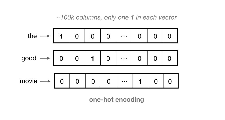
For large vocabularies, these vectors can get very long, and they contain all 0’s except for one value. This is considered a very sparse representation.

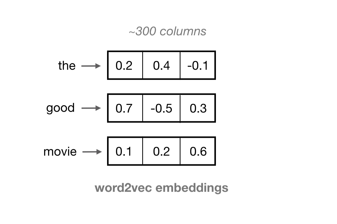
Word Embeddings (Word2Vec)

We often want a more dense representation. One such representation is a learned word vector, known as an embedding. Word embeddings are vectors of a specified length, typically on the order of 100, and each vector of 100 or so values, represents one word. The values in each column represent the features of a word, rather than any specific word.

These embeddings are formed in an unsupervised manner by training a single-layer neural network—a Word2Vec model—on an input word and a few surrounding words in a sentence.

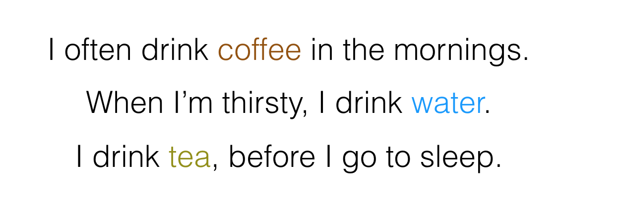
Words that show up in similar contexts (and have similar surrounding words), such as “coffee”, “tea”, and “water” will tend to have similar vectors; vectors that point in roughly the same direction. As such, similar words can be found by calculating the cosine similarity between word vectors and you can even add and subtract word vectors to do some interesting word math. If you’d like to learn more about Word2Vec, there are some wonderful resources out there, including this explanatory code example.

These word embeddings have some really nice properties:

• An embedding is a dense, vector representation of a word.
• Words that have similar contexts will tend to have embeddings that point in the same direction.

Similar to how we could encode a single review as a list of tokens, we can now represent a review as a list of word embeddings. These word embeddings can be used as input to a recurrent neural network or a convolutional neural network.

In the code associated with this post, I am going to use a pre-trained Word2Vec model to create word embeddings for a dataset of movie reviews.

Word2Vec and Embedded Bias

One thing to note about Word2Vec, is that, in addition to learning useful similarities and semantic relationships between words, these model also learn to represent problematic relationships between words. For example, a paper on Debiasing Word Embeddings by Bolukbasi et al. (2016), found that the vector-relationship between “man” and “woman” was similar to the relationship between “physician” and “registered nurse” or “shopkeeper” and “housewife” in the trained, Google News Word2Vec model, which I am using in my example implementation.

“In this paper, we quantitatively demonstrate that word-embeddings contain biases in their geometry that reflect gender stereotypes present in broader society. Due to their wide-spread usage as basic features, word embeddings not only reflect such stereotypes but can also amplify them. This poses a significant risk and challenge for machine learning and its applications.”

As such, it is important to note that my example code is using a Word2Vec model that has been shown to encapsulate gender stereotypes. I’d suggest reading this paper to learn about methods for debiasing word embeddings with respect to certain features; this is an ongoing area of research. Next, I will focus on using CNN’s for text classification.

Convolutional Kernels

Convolutional layers are designed to find spatial patterns in an image by sliding a small kernel window over an image. These windows are often small, perhaps 3×3 pixels in size, and each kernel cell has an associated weight. As a kernel slides over an image, pixel-by-pixel, the kernel weights are multiplied by the pixel value in the image underneath, then all the multiplied values are summed up to get an output, filtered pixel value. A detailed description of convolutional filters and convolutional neural networks can be found in a previous post if you’d like to learn more.

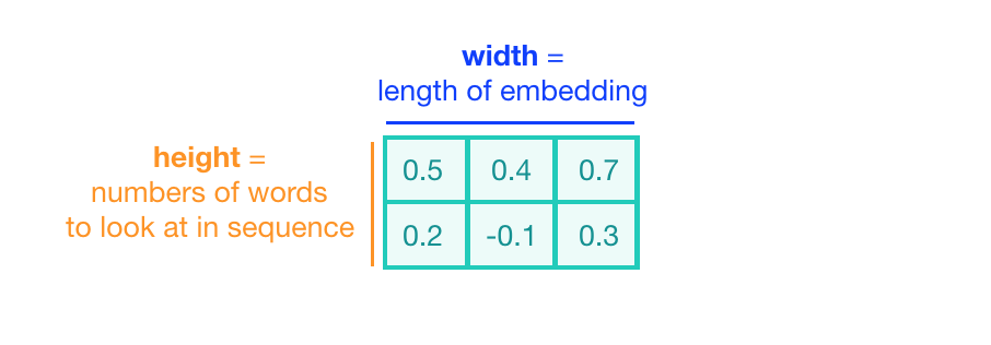
In the case of text classification, a convolutional kernel will still be a sliding window, only its job is to look at embeddings for multiple words, rather than small areas of pixels in an image. The dimensions of the convolutional kernel will also have to change, according to this task. To look at sequences of word embeddings, we want a window to look at multiple word embeddings in a sequence. The kernels will no longer be square, instead, they will be a wide rectangle with dimensions like 3×300 or 5×300 (assuming an embedding length of 300).

• The height of the kernel will be the number of embeddings it will see at once, similar to representing an n-gram in a word model.
• The width of the kernel should span the length of an entire word embedding.

Convolution over Word Sequences

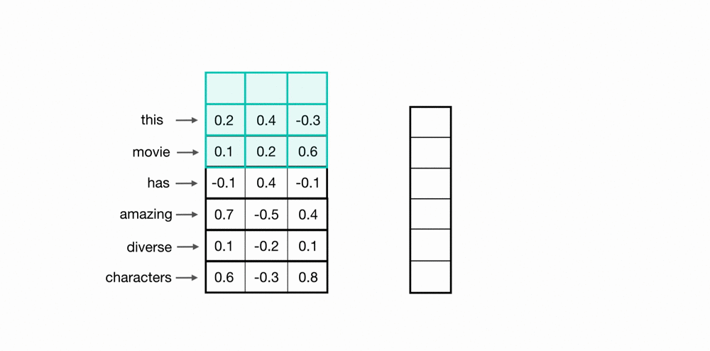
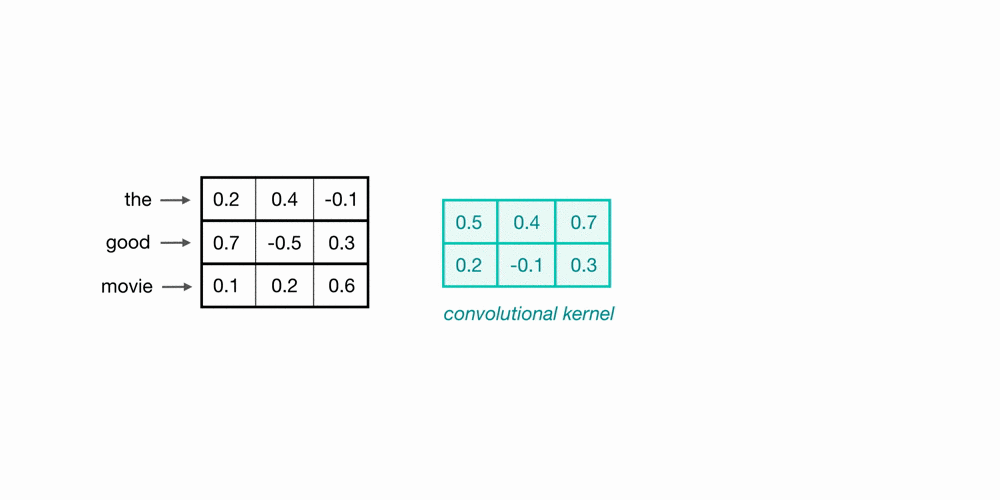
Let’s look at an example of what a pair (a 2-gram) of filtered word embeddings will look like. Below, we have a toy example that shows each word encoded as an embedding with 3 values, usually, this will contain many more values, but this is for ease of visualization.

To look at two words in this example sequence, we can use a 2×3 convolutional kernel. The kernel weights are placed on top of two word embeddings; in this case, the downwards-direction represents time, so, the word “movie” comes right after “good” in this short sequence. The kernel weights and embedding values are multiplied in pairs and then summed to get a single output value of 0.54.

A convolutional neural network will include many of these kernels, and, as the network trains, these kernel weights are learned. Each kernel is designed to look at a word, and surrounding word(s) in a sequential window, and output a value that captures something about that phrase. In this way, the convolution operation can be viewed as window-based feature extraction, where the features are patterns in sequential word groupings that indicate traits like the sentiment of a text, the grammatical function of different words, and so on.

It is also worth noting that the number of input channels for this convolutional layer—a value that is typically 1 for grayscale images or 3 for RGB images—will be 1 in this case, because a single, input text source will be encoded as one list of word embeddings.

Recognizing General Patterns

There is another nice property of this convolutional operation. Recall that similar words will have similar embeddings and a convolution operation is just a linear operation on these vectors. So, when a convolutional kernel is applied to different sets of similar words, it will produce a similar output value!

In the below example, you can see that the convolutional output value for the input 2-grams “good movie” and “fantastic song” are about the same because the word embeddings for those pairs of words are also very similar.

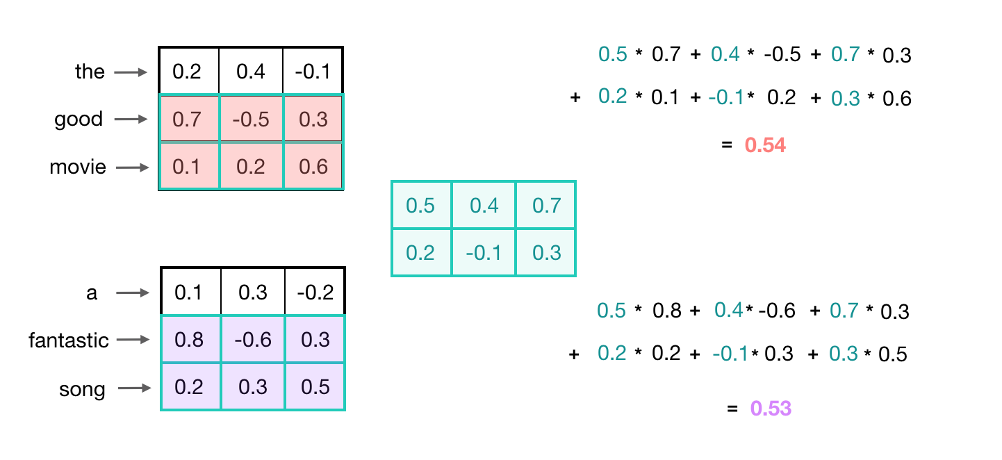
In this example, the convolutional kernel has learned to capture a more general feature; not just a good movie or song, but a positive thing, generally. Recognizing these kinds of high-level features can be especially useful in text classification tasks, which often rely on general groupings. For example, in sentiment analysis, a model would benefit from being able to represent negative, neutral, and positive word groupings. A model could use those general features to classify entire texts.

1D Convolutions

Now, you’ve seen how a convolutional kernel can be applied to a few word embeddings. To process an entire sequence of words, these kernels will slide down a list of word embeddings, in sequence. This is called a 1D convolution because the kernel is moving in only one dimension: time. A single kernel will move one-by-one down a list of input embeddings, looking at the first word embedding (and a small window of next-word embeddings) then the next word embedding, and the next, and so on. The resultant output will be a feature vector that contains about as many values as there were input embeddings, so the input sequence size does matter. I say “about” because sometimes a convolutional kernel will not perfectly overlay on the word embeddings and so some padding may need to be included to account for the height of the kernel. The relationship between padding and kernel size is described in more detail, in a previous post. Below, you can see what the output of a 1D convolution might look like when applied to a short sequence of word embeddings.

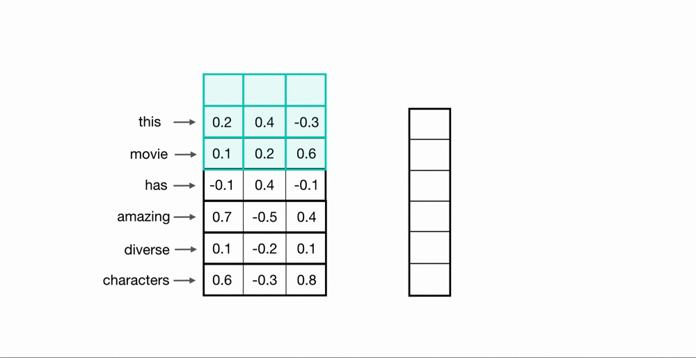
Multiple Kernels

Just like in a typical convolutional neural network, one convolutional kernel is not enough to detect all the different kinds of features that will be useful for a classification task. To set up a network so that it is capable of learning a variety of different relationships between words, you’ll need many filters of different heights. In the paper, Convolutional Neural Networks for Sentence Classification (Yoon Kim, 2014) they use 300 kernels total; 100 kernels for each height: 3, 4, and 5. These heights effectively capture patterns in sequential groups of 3, 4, and 5 words. They chose a cutoff of 5 words because words that were farther away than that were generally less relevant or useful with respect to identifying patterns in a phrase. For example, if I say “this apple is red and a banana is yellow” the words that are close together like ‘this’, ‘apple’, and ‘red’ are more related than far apart words like ‘apple’ and ‘yellow’. So, as a short, convolutional kernel slides over word embeddings, one at a time, it is designed to capture local features or features within a nearby window of sequential words. The stacked, output feature vectors that arise from several of these convolutional operations is called a convolutional layer.

Maxpooling over Time

Now, we’ve seen how a convolutional operation produces a feature vector that can represent local features in sequences of word embeddings. One thing to think about is how a feature vector might look when applied to an important phrase in a text source. If we are trying to classify movie reviews, and we see the phrase, “great plot,” it doesn’t matter where this appears in a review; it is a good indicator that this is a positive review, no matter its location in the source text.

In order to indicate the presence of these high-level features, we need a way to identify them in a vector, regardless of the location within the larger input sequence. One way to identify important features, no matter their location in a sequence, is to discard less-relevant, locational information. To do this, we can use a maxpooling operation, which forces the network to retain only the maximum value in a feature vector, which should be the most useful, local feature.

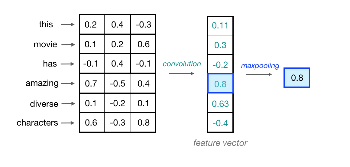
Since this operation is looking at a sequence of local feature values, it is often called maxpooling over time.

The max-values produced by processing each of our convolutional feature vectors will be concatenated and passed to a final, fully-connected layer that can produce as many class scores as a text classification task requires.

CNN for Text Classification: Complete Implementation

We’ve gone over a lot of information and now, I want to summarize by putting all of these concepts together.

• I’ve completed a readable, PyTorch implementation of a sentiment classification CNN that looks at movie reviews as input, and produces a class label (positive or negative) as output, based on the detected sentiment of the input text.

I encourage you to take a look at the complete notebook and look at how movie reviews are processed and what the complete model definition and training steps look like. The notebook includes the following steps:

1. Process all the movie reviews and their sentiment labels to remove outliers and encode the labels (positive=1, negative=0)
2. Load in a pre-trained Word2Vec model, and use it to tokenize each review
3. Pad and standardize each review so that input sequences are of the same length
4. Create training, validation, and test sets of data
5. Define and train a SentimentCNN model
6. Test the model on positive and negative reviews

The example code follows the structure outlined in the paper, Convolutional Neural Networks for Sentence Classification by Yoon Kim (2014). It shows how you can utilize convolutional layers to find patterns in sequences of word embeddings and create an effective text classifier using a CNN-based approach.

SentimentCNN

The complete network will see a batch of movie reviews as input. These go through a pre-trained embedding layer, then the sequences of word embeddings go through several convolutional operations, defined in my code as three convolutional layers with kernel heights of 3, 4, and 5. These layers go through a ReLu activation and maxpooling operation. Finally, the max-values from the three different convolutional layers are concatenated and passed to a final, fully-connected, classification layer.

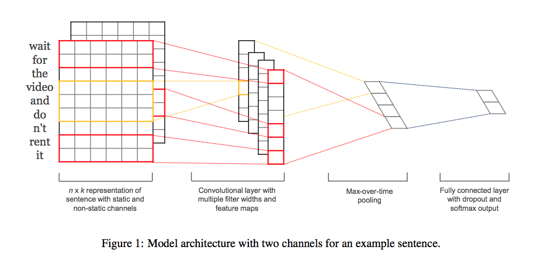
The above image was taken from the original Convolutional Neural Networks for Sentence Classification paper (Yoon Kim).

In my implementation, the classification layer is trained to output a single value, between 0 and 1, where close to 0 indicates a negative review and close to 1 indicates a positive review.

After this network trains, you can see how the trained model classifies some sample positive/negative reviews.

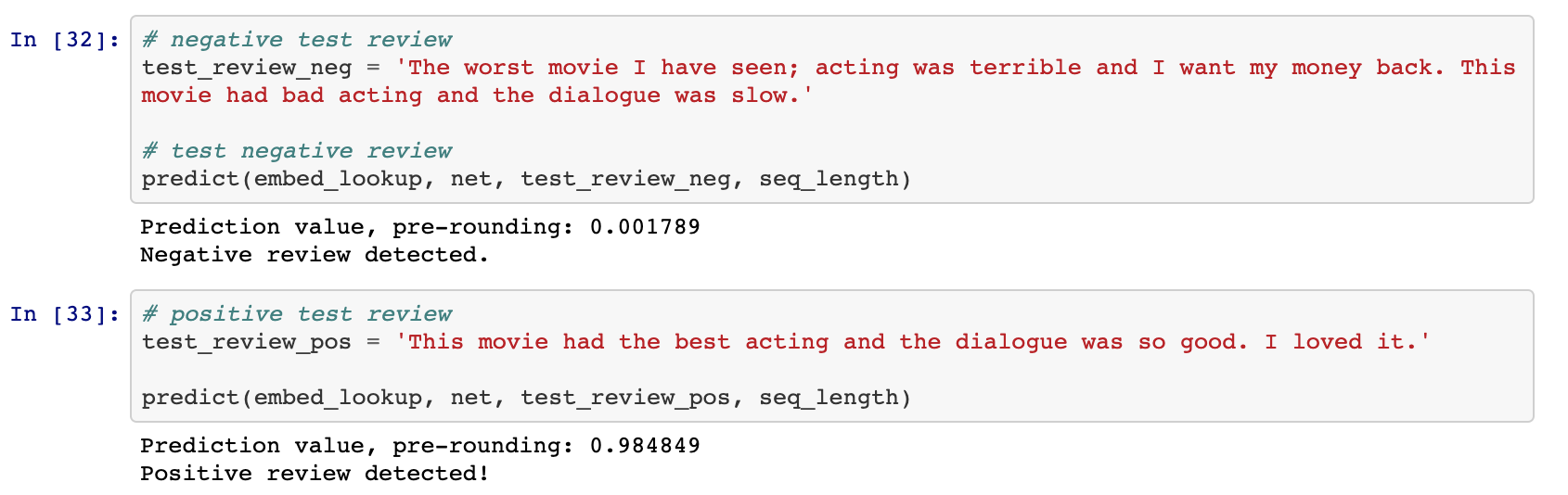
Further Learning

As I was writing the text classification code, I found that CNNs are used to analyze sequential data in a number of ways! Here are a couple of papers and applications that I found really interesting:

• CNN for semantic representations and search query retrieval, [paper (Microsoft)].
• CNN for genetic mutation detection, [paper (Nature)].
• CNN for classifying whale sounds via spectogram, [blog post (Google AI)].

I encourage you to read more and try to implement an application that interests you!

If you are interested in my work and thoughts, check out my Twitter or connect with me on LinkedIn.

wordEncoding

filename = "sonnetsPreprocessed.txt";
str = extractFileText(filename);
textData = split(str,newline);
documents = tokenizedDocument(textData);
documents(1:10)

ans = 
  10x1 tokenizedDocument:

    70 tokens: fairest creatures desire increase thereby beautys rose might never die riper time decease tender heir might bear memory thou contracted thine own bright eyes feedst thy lights flame selfsubstantial fuel making famine abundance lies thy self thy foe thy sweet self cruel thou art worlds fresh ornament herald gaudy spring thine own bud buriest thy content tender churl makst waste niggarding pity world else glutton eat worlds due grave thee
    71 tokens: forty winters shall besiege thy brow dig deep trenches thy beautys field thy youths proud livery gazed tatterd weed small worth held asked thy beauty lies treasure thy lusty days say thine own deep sunken eyes alleating shame thriftless praise praise deservd thy beautys thou couldst answer fair child mine shall sum count make old excuse proving beauty succession thine new made thou art old thy blood warm thou feelst cold
    65 tokens: look thy glass tell face thou viewest time face form another whose fresh repair thou renewest thou dost beguile world unbless mother fair whose uneard womb disdains tillage thy husbandry fond tomb selflove stop posterity thou art thy mothers glass thee calls back lovely april prime thou windows thine age shalt despite wrinkles thy golden time thou live rememberd die single thine image dies thee
    71 tokens: unthrifty loveliness why dost thou spend upon thy self thy beautys legacy natures bequest gives nothing doth lend frank lends free beauteous niggard why dost thou abuse bounteous largess thee give profitless usurer why dost thou great sum sums yet canst live traffic thy self alone thou thy self thy sweet self dost deceive nature calls thee gone acceptable audit canst thou leave thy unused beauty tombed thee lives th executor
    61 tokens: hours gentle work frame lovely gaze every eye doth dwell play tyrants same unfair fairly doth excel neverresting time leads summer hideous winter confounds sap checked frost lusty leaves quite gone beauty oersnowed bareness every summers distillation left liquid prisoner pent walls glass beautys effect beauty bereft nor nor remembrance flowers distilld though winter meet leese show substance still lives sweet
    68 tokens: let winters ragged hand deface thee thy summer ere thou distilld make sweet vial treasure thou place beautys treasure ere selfkilld forbidden usury happies pay willing loan thats thy self breed another thee ten times happier ten ten times thy self happier thou art ten thine ten times refigurd thee death thou shouldst depart leaving thee living posterity selfwilld thou art fair deaths conquest make worms thine heir
    64 tokens: lo orient gracious light lifts up burning head eye doth homage newappearing sight serving looks sacred majesty climbd steepup heavenly hill resembling strong youth middle age yet mortal looks adore beauty still attending golden pilgrimage highmost pitch weary car like feeble age reeleth day eyes fore duteous converted low tract look another way thou thyself outgoing thy noon unlookd diest unless thou get son
    70 tokens: music hear why hearst thou music sadly sweets sweets war joy delights joy why lovst thou thou receivst gladly else receivst pleasure thine annoy true concord welltuned sounds unions married offend thine ear sweetly chide thee confounds singleness parts thou shouldst bear mark string sweet husband another strikes mutual ordering resembling sire child happy mother pleasing note sing whose speechless song many seeming sings thee thou single wilt prove none
    70 tokens: fear wet widows eye thou consumst thy self single life ah thou issueless shalt hap die world wail thee like makeless wife world thy widow still weep thou form thee hast left behind every private widow well keep childrens eyes husbands shape mind look unthrift world doth spend shifts place still world enjoys beautys waste hath world end kept unused user destroys love toward others bosom sits murdrous shame commits
    69 tokens: shame deny thou bearst love thy self art unprovident grant thou wilt thou art belovd many thou none lovst evident thou art possessd murderous hate gainst thy self thou stickst conspire seeking beauteous roof ruinate repair thy chief desire o change thy thought change mind shall hate fairer lodgd gentle love thy presence gracious kind thyself least kindhearted prove make thee another self love beauty still live thine thee

enc = wordEncoding(documents)

enc = 
  wordEncoding with properties:

      NumWords: 3092
    Vocabulary: ["fairest"    "creatures"    "desire"    "increase"    "thereby"    "beautys"    "rose"    "might"    "never"    "die"    "riper"    "time"    "decease"    "tender"    "heir"    "bear"    "memory"    "thou"    "contracted"    ...    ]

emb = fastTextWordEmbedding;

enc = wordEncoding(words)

enc = 
  wordEncoding with properties:

      NumWords: 999994
    Vocabulary: [1×999994 string]

dimension = emb.Dimension;
numWords = numel(words);

layer = wordEmbeddingLayer(dimension,numWords, ...
    'Weights',word2vec(emb,words)')

layer = 
  WordEmbeddingLayer with properties:

         Name: ''

   Hyperparameters
    Dimension: 300
     NumWords: 999994

   Learnable Parameters
      Weights: [300×999994 single]

  Show all properties

filename = "sonnetsPreprocessed.txt";
str = extractFileText(filename);
textData = split(str,newline);
documents = tokenizedDocument(textData);
documents(1:10)

ans = 
  10x1 tokenizedDocument:

    70 tokens: fairest creatures desire increase thereby beautys rose might never die riper time decease tender heir might bear memory thou contracted thine own bright eyes feedst thy lights flame selfsubstantial fuel making famine abundance lies thy self thy foe thy sweet self cruel thou art worlds fresh ornament herald gaudy spring thine own bud buriest thy content tender churl makst waste niggarding pity world else glutton eat worlds due grave thee
    71 tokens: forty winters shall besiege thy brow dig deep trenches thy beautys field thy youths proud livery gazed tatterd weed small worth held asked thy beauty lies treasure thy lusty days say thine own deep sunken eyes alleating shame thriftless praise praise deservd thy beautys thou couldst answer fair child mine shall sum count make old excuse proving beauty succession thine new made thou art old thy blood warm thou feelst cold
    65 tokens: look thy glass tell face thou viewest time face form another whose fresh repair thou renewest thou dost beguile world unbless mother fair whose uneard womb disdains tillage thy husbandry fond tomb selflove stop posterity thou art thy mothers glass thee calls back lovely april prime thou windows thine age shalt despite wrinkles thy golden time thou live rememberd die single thine image dies thee
    71 tokens: unthrifty loveliness why dost thou spend upon thy self thy beautys legacy natures bequest gives nothing doth lend frank lends free beauteous niggard why dost thou abuse bounteous largess thee give profitless usurer why dost thou great sum sums yet canst live traffic thy self alone thou thy self thy sweet self dost deceive nature calls thee gone acceptable audit canst thou leave thy unused beauty tombed thee lives th executor
    61 tokens: hours gentle work frame lovely gaze every eye doth dwell play tyrants same unfair fairly doth excel neverresting time leads summer hideous winter confounds sap checked frost lusty leaves quite gone beauty oersnowed bareness every summers distillation left liquid prisoner pent walls glass beautys effect beauty bereft nor nor remembrance flowers distilld though winter meet leese show substance still lives sweet
    68 tokens: let winters ragged hand deface thee thy summer ere thou distilld make sweet vial treasure thou place beautys treasure ere selfkilld forbidden usury happies pay willing loan thats thy self breed another thee ten times happier ten ten times thy self happier thou art ten thine ten times refigurd thee death thou shouldst depart leaving thee living posterity selfwilld thou art fair deaths conquest make worms thine heir
    64 tokens: lo orient gracious light lifts up burning head eye doth homage newappearing sight serving looks sacred majesty climbd steepup heavenly hill resembling strong youth middle age yet mortal looks adore beauty still attending golden pilgrimage highmost pitch weary car like feeble age reeleth day eyes fore duteous converted low tract look another way thou thyself outgoing thy noon unlookd diest unless thou get son
    70 tokens: music hear why hearst thou music sadly sweets sweets war joy delights joy why lovst thou thou receivst gladly else receivst pleasure thine annoy true concord welltuned sounds unions married offend thine ear sweetly chide thee confounds singleness parts thou shouldst bear mark string sweet husband another strikes mutual ordering resembling sire child happy mother pleasing note sing whose speechless song many seeming sings thee thou single wilt prove none
    70 tokens: fear wet widows eye thou consumst thy self single life ah thou issueless shalt hap die world wail thee like makeless wife world thy widow still weep thou form thee hast left behind every private widow well keep childrens eyes husbands shape mind look unthrift world doth spend shifts place still world enjoys beautys waste hath world end kept unused user destroys love toward others bosom sits murdrous shame commits
    69 tokens: shame deny thou bearst love thy self art unprovident grant thou wilt thou art belovd many thou none lovst evident thou art possessd murderous hate gainst thy self thou stickst conspire seeking beauteous roof ruinate repair thy chief desire o change thy thought change mind shall hate fairer lodgd gentle love thy presence gracious kind thyself least kindhearted prove make thee another self love beauty still live thine thee

enc = wordEncoding(documents, ...
    'Order','frequency', ...
    'MaxNumWords',100)

enc = 
  wordEncoding with properties:

      NumWords: 100
    Vocabulary: ["thy"    "thou"    "love"    "thee"    "doth"    "mine"    "shall"    "eyes"    "sweet"    "time"    "beauty"    "nor"    "art"    "yet"    "o"    "heart"    "thine"    "fair"    "make"    "hath"    "still"    "eye"    "true"    ...    ]

idx = [1 2 3];
words = ind2word(enc,idx)

words = 1x3 string
    "thy"    "thou"    "love"

filename = "sonnetsPreprocessed.txt";
str = extractFileText(filename);
textData = split(str,newline);
documents = tokenizedDocument(textData);
documents(1:10)

ans = 
  10x1 tokenizedDocument:

    70 tokens: fairest creatures desire increase thereby beautys rose might never die riper time decease tender heir might bear memory thou contracted thine own bright eyes feedst thy lights flame selfsubstantial fuel making famine abundance lies thy self thy foe thy sweet self cruel thou art worlds fresh ornament herald gaudy spring thine own bud buriest thy content tender churl makst waste niggarding pity world else glutton eat worlds due grave thee
    71 tokens: forty winters shall besiege thy brow dig deep trenches thy beautys field thy youths proud livery gazed tatterd weed small worth held asked thy beauty lies treasure thy lusty days say thine own deep sunken eyes alleating shame thriftless praise praise deservd thy beautys thou couldst answer fair child mine shall sum count make old excuse proving beauty succession thine new made thou art old thy blood warm thou feelst cold
    65 tokens: look thy glass tell face thou viewest time face form another whose fresh repair thou renewest thou dost beguile world unbless mother fair whose uneard womb disdains tillage thy husbandry fond tomb selflove stop posterity thou art thy mothers glass thee calls back lovely april prime thou windows thine age shalt despite wrinkles thy golden time thou live rememberd die single thine image dies thee
    71 tokens: unthrifty loveliness why dost thou spend upon thy self thy beautys legacy natures bequest gives nothing doth lend frank lends free beauteous niggard why dost thou abuse bounteous largess thee give profitless usurer why dost thou great sum sums yet canst live traffic thy self alone thou thy self thy sweet self dost deceive nature calls thee gone acceptable audit canst thou leave thy unused beauty tombed thee lives th executor
    61 tokens: hours gentle work frame lovely gaze every eye doth dwell play tyrants same unfair fairly doth excel neverresting time leads summer hideous winter confounds sap checked frost lusty leaves quite gone beauty oersnowed bareness every summers distillation left liquid prisoner pent walls glass beautys effect beauty bereft nor nor remembrance flowers distilld though winter meet leese show substance still lives sweet
    68 tokens: let winters ragged hand deface thee thy summer ere thou distilld make sweet vial treasure thou place beautys treasure ere selfkilld forbidden usury happies pay willing loan thats thy self breed another thee ten times happier ten ten times thy self happier thou art ten thine ten times refigurd thee death thou shouldst depart leaving thee living posterity selfwilld thou art fair deaths conquest make worms thine heir
    64 tokens: lo orient gracious light lifts up burning head eye doth homage newappearing sight serving looks sacred majesty climbd steepup heavenly hill resembling strong youth middle age yet mortal looks adore beauty still attending golden pilgrimage highmost pitch weary car like feeble age reeleth day eyes fore duteous converted low tract look another way thou thyself outgoing thy noon unlookd diest unless thou get son
    70 tokens: music hear why hearst thou music sadly sweets sweets war joy delights joy why lovst thou thou receivst gladly else receivst pleasure thine annoy true concord welltuned sounds unions married offend thine ear sweetly chide thee confounds singleness parts thou shouldst bear mark string sweet husband another strikes mutual ordering resembling sire child happy mother pleasing note sing whose speechless song many seeming sings thee thou single wilt prove none
    70 tokens: fear wet widows eye thou consumst thy self single life ah thou issueless shalt hap die world wail thee like makeless wife world thy widow still weep thou form thee hast left behind every private widow well keep childrens eyes husbands shape mind look unthrift world doth spend shifts place still world enjoys beautys waste hath world end kept unused user destroys love toward others bosom sits murdrous shame commits
    69 tokens: shame deny thou bearst love thy self art unprovident grant thou wilt thou art belovd many thou none lovst evident thou art possessd murderous hate gainst thy self thou stickst conspire seeking beauteous roof ruinate repair thy chief desire o change thy thought change mind shall hate fairer lodgd gentle love thy presence gracious kind thyself least kindhearted prove make thee another self love beauty still live thine thee

enc = wordEncoding(documents)

enc = 
  wordEncoding with properties:

      NumWords: 3092
    Vocabulary: ["fairest"    "creatures"    "desire"    "increase"    "thereby"    "beautys"    "rose"    "might"    "never"    "die"    "riper"    "time"    "decease"    "tender"    "heir"    "bear"    "memory"    "thou"    "contracted"    ...    ]

idx = [1 3 5];
words = ind2word(enc,idx)

words = 1x3 string
    "fairest"    "desire"    "thereby"

filename = "sonnetsPreprocessed.txt";
str = extractFileText(filename);
textData = split(str,newline);
documents = tokenizedDocument(textData);
documents(1:10)

ans = 
  10x1 tokenizedDocument:

    70 tokens: fairest creatures desire increase thereby beautys rose might never die riper time decease tender heir might bear memory thou contracted thine own bright eyes feedst thy lights flame selfsubstantial fuel making famine abundance lies thy self thy foe thy sweet self cruel thou art worlds fresh ornament herald gaudy spring thine own bud buriest thy content tender churl makst waste niggarding pity world else glutton eat worlds due grave thee
    71 tokens: forty winters shall besiege thy brow dig deep trenches thy beautys field thy youths proud livery gazed tatterd weed small worth held asked thy beauty lies treasure thy lusty days say thine own deep sunken eyes alleating shame thriftless praise praise deservd thy beautys thou couldst answer fair child mine shall sum count make old excuse proving beauty succession thine new made thou art old thy blood warm thou feelst cold
    65 tokens: look thy glass tell face thou viewest time face form another whose fresh repair thou renewest thou dost beguile world unbless mother fair whose uneard womb disdains tillage thy husbandry fond tomb selflove stop posterity thou art thy mothers glass thee calls back lovely april prime thou windows thine age shalt despite wrinkles thy golden time thou live rememberd die single thine image dies thee
    71 tokens: unthrifty loveliness why dost thou spend upon thy self thy beautys legacy natures bequest gives nothing doth lend frank lends free beauteous niggard why dost thou abuse bounteous largess thee give profitless usurer why dost thou great sum sums yet canst live traffic thy self alone thou thy self thy sweet self dost deceive nature calls thee gone acceptable audit canst thou leave thy unused beauty tombed thee lives th executor
    61 tokens: hours gentle work frame lovely gaze every eye doth dwell play tyrants same unfair fairly doth excel neverresting time leads summer hideous winter confounds sap checked frost lusty leaves quite gone beauty oersnowed bareness every summers distillation left liquid prisoner pent walls glass beautys effect beauty bereft nor nor remembrance flowers distilld though winter meet leese show substance still lives sweet
    68 tokens: let winters ragged hand deface thee thy summer ere thou distilld make sweet vial treasure thou place beautys treasure ere selfkilld forbidden usury happies pay willing loan thats thy self breed another thee ten times happier ten ten times thy self happier thou art ten thine ten times refigurd thee death thou shouldst depart leaving thee living posterity selfwilld thou art fair deaths conquest make worms thine heir
    64 tokens: lo orient gracious light lifts up burning head eye doth homage newappearing sight serving looks sacred majesty climbd steepup heavenly hill resembling strong youth middle age yet mortal looks adore beauty still attending golden pilgrimage highmost pitch weary car like feeble age reeleth day eyes fore duteous converted low tract look another way thou thyself outgoing thy noon unlookd diest unless thou get son
    70 tokens: music hear why hearst thou music sadly sweets sweets war joy delights joy why lovst thou thou receivst gladly else receivst pleasure thine annoy true concord welltuned sounds unions married offend thine ear sweetly chide thee confounds singleness parts thou shouldst bear mark string sweet husband another strikes mutual ordering resembling sire child happy mother pleasing note sing whose speechless song many seeming sings thee thou single wilt prove none
    70 tokens: fear wet widows eye thou consumst thy self single life ah thou issueless shalt hap die world wail thee like makeless wife world thy widow still weep thou form thee hast left behind every private widow well keep childrens eyes husbands shape mind look unthrift world doth spend shifts place still world enjoys beautys waste hath world end kept unused user destroys love toward others bosom sits murdrous shame commits
    69 tokens: shame deny thou bearst love thy self art unprovident grant thou wilt thou art belovd many thou none lovst evident thou art possessd murderous hate gainst thy self thou stickst conspire seeking beauteous roof ruinate repair thy chief desire o change thy thought change mind shall hate fairer lodgd gentle love thy presence gracious kind thyself least kindhearted prove make thee another self love beauty still live thine thee

enc = wordEncoding(documents)

enc = 
  wordEncoding with properties:

      NumWords: 3092
    Vocabulary: ["fairest"    "creatures"    "desire"    "increase"    "thereby"    "beautys"    "rose"    "might"    "never"    "die"    "riper"    "time"    "decease"    "tender"    "heir"    "bear"    "memory"    "thou"    "contracted"    ...    ]

words = ["rose" "love" "beauty"];
idx = word2ind(enc,words)

filename = "factoryReports.csv";
data = readtable(filename,'TextType','string');
textData = data.Description;
documents = tokenizedDocument(textData);

enc = wordEncoding(documents);

sequences = doc2sequence(enc,documents);

ans=10×1 cell array
    {[           0 0 0 0 0 0 0 1 2 3 4 5 6 7 8 9 10]}
    {[  0 0 0 0 0 0 11 12 13 14 15 2 16 17 18 19 10]}
    {[    0 0 0 0 0 0 20 2 21 22 7 23 24 25 7 26 10]}
    {[        0 0 0 0 0 0 0 0 0 0 0 27 28 6 7 18 10]}
    {[        0 0 0 0 0 0 0 0 0 0 0 0 29 30 7 31 10]}
    {[    0 0 0 0 0 0 0 32 33 6 7 34 35 36 37 38 10]}
    {[      0 0 0 0 0 0 0 0 0 39 40 36 41 6 7 42 10]}
    {[    0 0 0 0 0 0 0 0 43 44 22 45 46 47 7 48 10]}
    {[      0 0 0 0 0 0 0 0 0 0 49 50 17 7 51 48 10]}
    {[0 0 0 0 52 8 53 36 54 55 56 57 58 59 22 60 10]}