Editing links in excel - Word и Excel - помощь в работе с программами

For quick access to related information in another file or on a web page, you can insert a hyperlink in a worksheet cell. You can also insert links in specific chart elements.

Note: Most of the screen shots in this article were taken in Excel 2016. If you have a different version your view might be slightly different, but unless otherwise noted, the functionality is the same.

On a worksheet, click the cell where you want to create a link.

You can also select an object, such as a picture or an element in a chart, that you want to use to represent the link.
- On the Insert tab, in the Links group, click Link .
You can also right-click the cell or graphic and then click Link on the shortcut menu, or you can press Ctrl+K.
Under Link to, click Create New Document.
In the Name of new document box, type a name for the new file.

Tip: To specify a location other than the one shown under Full path, you can type the new location preceding the name in the Name of new document box, or you can click Change to select the location that you want and then click OK.
Under When to edit, click Edit the new document later or Edit the new document now to specify when you want to open the new file for editing.
In the Text to display box, type the text that you want to use to represent the link.
To display helpful information when you rest the pointer on the link, click ScreenTip, type the text that you want in the ScreenTip text box, and then click OK.

On a worksheet, click the cell where you want to create a link.

You can also select an object, such as a picture or an element in a chart, that you want to use to represent the link.
- On the Insert tab, in the Links group, click Link .
You can also right-click the cell or object and then click Link on the shortcut menu, or you can press Ctrl+K.
Under Link to, click Existing File or Web Page.
Do one of the following:
- To select a file, click Current Folder, and then click the file that you want to link to.
  
  You can change the current folder by selecting a different folder in the Look in list.
- To select a web page, click Browsed Pages and then click the web page that you want to link to.
- To select a file that you recently used, click Recent Files, and then click the file that you want to link to.
- To enter the name and location of a known file or web page that you want to link to, type that information in the Address box.
- To locate a web page, click Browse the Web , open the web page that you want to link to, and then switch back to Excel without closing your browser.
If you want to create a link to a specific location in the file or on the web page, click Bookmark, and then double-click the bookmark that you want.

Note: The file or web page that you are linking to must have a bookmark.
In the Text to display box, type the text that you want to use to represent the link.
To display helpful information when you rest the pointer on the link, click ScreenTip, type the text that you want in the ScreenTip text box, and then click OK.

To link to a location in the current workbook or another workbook, you can either define a name for the destination cells or use a cell reference.

To use a name, you must name the destination cells in the destination workbook.

How to name a cell or a range of cells
1. Select the cell, range of cells, or nonadjacent selections that you want to name.
2. Click the Name box at the left end of the formula bar .
  
  Name box
3. In the Name box, type the name for the cells, and then press Enter.
  
  Note: Names can’t contain spaces and must begin with a letter.
On a worksheet of the source workbook, click the cell where you want to create a link.

You can also select an object, such as a picture or an element in a chart, that you want to use to represent the link.
- On the Insert tab, in the Links group, click Link .
You can also right-click the cell or object and then click Link on the shortcut menu, or you can press Ctrl+K.
Under Link to, do one of the following:
- To link to a location in your current workbook, click Place in This Document.
- To link to a location in another workbook, click Existing File or Web Page, locate and select the workbook that you want to link to, and then click Bookmark.
Do one of the following:
- In the Or select a place in this document box, under Cell Reference, click the worksheet that you want to link to, type the cell reference in the Type in the cell reference box, and then click OK.
- In the list under Defined Names, click the name that represents the cells that you want to link to, and then click OK.
In the Text to display box, type the text that you want to use to represent the link.
To display helpful information when you rest the pointer on the link, click ScreenTip, type the text that you want in the ScreenTip text box, and then click OK.

You can use the HYPERLINK function to create a link that opens a document that is stored on a network server, an intranet, or the Internet. When you click the cell that contains the HYPERLINK function, Excel opens the file that is stored at the location of the link.

Syntax

HYPERLINK(link_location,friendly_name)

Link_location is the path and file name to the document to be opened as text. Link_location can refer to a place in a document — such as a specific cell or named range in an Excel worksheet or workbook, or to a bookmark in a Microsoft Word document. The path can be to a file stored on a hard disk drive, or the path can be a universal naming convention (UNC) path on a server (in Microsoft Excel for Windows) or a Uniform Resource Locator (URL) path on the Internet or an intranet.

Link_location can be a text string enclosed in quotation marks or a cell that contains the link as a text string.
If the jump specified in link_location does not exist or can’t be navigated, an error appears when you click the cell.

Friendly_name is the jump text or numeric value that is displayed in the cell. Friendly_name is displayed in blue and is underlined. If friendly_name is omitted, the cell displays the link_location as the jump text.

Friendly_name can be a value, a text string, a name, or a cell that contains the jump text or value.
If friendly_name returns an error value (for example, #VALUE!), the cell displays the error instead of the jump text.

Examples

The following example opens a worksheet named Budget Report.xls that is stored on the Internet at the location named example.microsoft.com/report and displays the text «Click for report»:

=HYPERLINK(«http://example.microsoft.com/report/budget report.xls», «Click for report»)

The following example creates a link to cell F10 on the worksheet named Annual in the workbook Budget Report.xls, which is stored on the Internet at the location named example.microsoft.com/report. The cell on the worksheet that contains the link displays the contents of cell D1 as the jump text:

=HYPERLINK(«[http://example.microsoft.com/report/budget report.xls]Annual!F10», D1)

The following example creates a link to the range named DeptTotal on the worksheet named First Quarter in the workbook Budget Report.xls, which is stored on the Internet at the location named example.microsoft.com/report. The cell on the worksheet that contains the link displays the text «Click to see First Quarter Department Total»:

=HYPERLINK(«[http://example.microsoft.com/report/budget report.xls]First Quarter!DeptTotal», «Click to see First Quarter Department Total»)

To create a link to a specific location in a Microsoft Word document, you must use a bookmark to define the location you want to jump to in the document. The following example creates a link to the bookmark named QrtlyProfits in the document named Annual Report.doc located at example.microsoft.com:

=HYPERLINK(«[http://example.microsoft.com/Annual Report.doc]QrtlyProfits», «Quarterly Profit Report»)

In Excel for Windows, the following example displays the contents of cell D5 as the jump text in the cell and opens the file named 1stqtr.xls, which is stored on the server named FINANCE in the Statements share. This example uses a UNC path:

=HYPERLINK(«\FINANCEStatements1stqtr.xls», D5)

The following example opens the file 1stqtr.xls in Excel for Windows that is stored in a directory named Finance on drive D, and displays the numeric value stored in cell H10:

=HYPERLINK(«D:FINANCE1stqtr.xls», H10)

In Excel for Windows, the following example creates a link to the area named Totals in another (external) workbook, Mybook.xls:

=HYPERLINK(«[C:My DocumentsMybook.xls]Totals»)

In Microsoft Excel for the Macintosh, the following example displays «Click here» in the cell and opens the file named First Quarter that is stored in a folder named Budget Reports on the hard drive named Macintosh HD:

=HYPERLINK(«Macintosh HD:Budget Reports:First Quarter», «Click here»)

You can create links within a worksheet to jump from one cell to another cell. For example, if the active worksheet is the sheet named June in the workbook named Budget, the following formula creates a link to cell E56. The link text itself is the value in cell E56.

=HYPERLINK(«[Budget]June!E56», E56)

To jump to a different sheet in the same workbook, change the name of the sheet in the link. In the previous example, to create a link to cell E56 on the September sheet, change the word «June» to «September.»

When you click a link to an email address, your email program automatically starts and creates an email message with the correct address in the To box, provided that you have an email program installed.

On a worksheet, click the cell where you want to create a link.

You can also select an object, such as a picture or an element in a chart, that you want to use to represent the link.
- On the Insert tab, in the Links group, click Link .
You can also right-click the cell or object and then click Link on the shortcut menu, or you can press Ctrl+K.
Under Link to, click E-mail Address.
In the E-mail address box, type the email address that you want.
In the Subject box, type the subject of the email message.

Note: Some web browsers and email programs may not recognize the subject line.
In the Text to display box, type the text that you want to use to represent the link.
To display helpful information when you rest the pointer on the link, click ScreenTip, type the text that you want in the ScreenTip text box, and then click OK.

You can also create a link to an email address in a cell by typing the address directly in the cell. For example, a link is created automatically when you type an email address, such as someone@example.com.

You can insert one or more external reference (also called links) from a workbook to another workbook that is located on your intranet or on the Internet. The workbook must not be saved as an HTML file.

Open the source workbook and select the cell or cell range that you want to copy.
On the Home tab, in the Clipboard group, click Copy.
Switch to the worksheet that you want to place the information in, and then click the cell where you want the information to appear.
On the Home tab, in the Clipboard group, click Paste Special.
Click Paste Link.

Excel creates an external reference link for the cell or each cell in the cell range.

Note: You may find it more convenient to create an external reference link without opening the workbook on the web. For each cell in the destination workbook where you want the external reference link, click the cell, and then type an equal sign (=), the URL address, and the location in the workbook. For example:

=’http://www.someones.homepage/[file.xls]Sheet1′!A1

=’ftp.server.somewhere/file.xls’!MyNamedCell

To select a hyperlink without activating the link to its destination, do one of the following:

Click the cell that contains the link, hold the mouse button until the pointer becomes a cross , and then release the mouse button.
Use the arrow keys to select the cell that contains the link.
If the link is represented by a graphic, hold down Ctrl, and then click the graphic.

You can change an existing link in your workbook by changing its destination, its appearance, or the text or graphic that is used to represent it.

Change the destination of a link

Select the cell or graphic that contains the link that you want to change.

Tip: To select a cell that contains a link without going to the link destination, click the cell and hold the mouse button until the pointer becomes a cross , and then release the mouse button. You can also use the arrow keys to select the cell. To select a graphic, hold down Ctrl and click the graphic.
- On the Insert tab, in the Links group, click Link.
You can also right-click the cell or graphic and then click Edit Link on the shortcut menu, or you can press Ctrl+K.
In the Edit Hyperlink dialog box, make the changes that you want.

Note: If the link was created by using the HYPERLINK worksheet function, you must edit the formula to change the destination. Select the cell that contains the link, and then click the formula bar to edit the formula.

You can change the appearance of all link text in the current workbook by changing the cell style for links.

On the Home tab, in the Styles group, click Cell Styles.
Under Data and Model, do the following:
- To change the appearance of links that have not been clicked to go to their destinations, right-click Link, and then click Modify.
- To change the appearance of links that have been clicked to go to their destinations, right-click Followed Link, and then click Modify.
  
  Note: The Link cell style is available only when the workbook contains a link. The Followed Link cell style is available only when the workbook contains a link that has been clicked.
In the Style dialog box, click Format.
On the Font tab and Fill tab, select the formatting options that you want, and then click OK.
Notes:
- The options that you select in the Format Cells dialog box appear as selected under Style includes in the Style dialog box. You can clear the check boxes for any options that you don’t want to apply.
- Changes that you make to the Link and Followed Link cell styles apply to all links in the current workbook. You can’t change the appearance of individual links.

Select the cell or graphic that contains the link that you want to change.

Tip: To select a cell that contains a link without going to the link destination, click the cell and hold the mouse button until the pointer becomes a cross , and then release the mouse button. You can also use the arrow keys to select the cell. To select a graphic, hold down Ctrl and click the graphic.
Do one or more of the following:
- To change the link text, click in the formula bar, and then edit the text.
- To change the format of a graphic, right-click it, and then click the option that you need to change its format.
- To change text in a graphic, double-click the selected graphic, and then make the changes that you want.
- To change the graphic that represents the link, insert a new graphic, make it a link with the same destination, and then delete the old graphic and link.

Right-click the hyperlink that you want to copy or move, and then click Copy or Cut on the shortcut menu.
Right-click the cell that you want to copy or move the link to, and then click Paste on the shortcut menu.

By default, unspecified paths to hyperlink destination files are relative to the location of the active workbook. Use this procedure when you want to set a different default path. Each time that you create a link to a file in that location, you only have to specify the file name, not the path, in the Insert Hyperlink dialog box.

Follow one of the steps depending on the Excel version you are using:

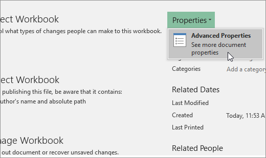
In Excel 2016, Excel 2013, and Excel 2010:
1. Click the File tab.
2. Click Info.
3. Click Properties, and then select Advanced Properties.
4. In the Summary tab, in the Hyperlink base text box, type the path that you want to use.
  
  Note: You can override the link base address by using the full, or absolute, address for the link in the Insert Hyperlink dialog box.
In Excel 2007:
1. Click the Microsoft Office Button , click Prepare, and then click Properties.
2. In the Document Information Panel, click Properties, and then click Advanced Properties.
3. Click the Summary tab.
4. In the Hyperlink base box, type the path that you want to use.
Note: You can override the link base address by using the full, or absolute, address for the link in the Insert Hyperlink dialog box.

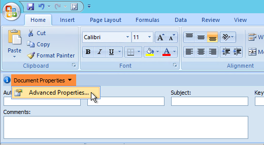
To delete a link, do one of the following:

To delete a link and the text that represents it, right-click the cell that contains the link, and then click Clear Contents on the shortcut menu.
To delete a link and the graphic that represents it, hold down Ctrl and click the graphic, and then press Delete.
To turn off a single link, right-click the link, and then click Remove Link on the shortcut menu.
To turn off several links at once, do the following:
1. In a blank cell, type the number 1.
2. Right-click the cell, and then click Copy on the shortcut menu.
3. Hold down Ctrl and select each link that you want to turn off.
  
  Tip: To select a cell that has a link in it without going to the link destination, click the cell and hold the mouse button until the pointer becomes a cross , and then release the mouse button.
4. On the Home tab, in the Clipboard group, click the arrow below Paste, and then click Paste Special.
5. Under Operation, click Multiply, and then click OK.
6. On the Home tab, in the Styles group, click Cell Styles.
7. Under Good, Bad, and Neutral, select Normal.

A link opens another page or file when you click it. The destination is frequently another web page, but it can also be a picture, or an email address, or a program. The link itself can be text or a picture.

When a site user clicks the link, the destination is shown in a Web browser, opened, or run, depending on the type of destination. For example, a link to a page shows the page in the web browser, and a link to an AVI file opens the file in a media player.

How links are used

You can use links to do the following:

Navigate to a file or web page on a network, intranet, or Internet
Navigate to a file or web page that you plan to create in the future
Send an email message
Start a file transfer, such as downloading or an FTP process

When you point to text or a picture that contains a link, the pointer becomes a hand , indicating that the text or picture is something that you can click.

What a URL is and how it works

When you create a link, its destination is encoded as a Uniform Resource Locator (URL), such as:

http://example.microsoft.com/news.htm

file://ComputerName/SharedFolder/FileName.htm

A URL contains a protocol, such as HTTP, FTP, or FILE, a Web server or network location, and a path and file name. The following illustration defines the parts of the URL:

1. Protocol used (http, ftp, file)

2. Web server or network location

3. Path

4. File name

Absolute and relative links

An absolute URL contains a full address, including the protocol, the Web server, and the path and file name.

A relative URL has one or more missing parts. The missing information is taken from the page that contains the URL. For example, if the protocol and web server are missing, the web browser uses the protocol and domain, such as .com, .org, or .edu, of the current page.

It is common for pages on the web to use relative URLs that contain only a partial path and file name. If the files are moved to another server, any links will continue to work as long as the relative positions of the pages remain unchanged. For example, a link on Products.htm points to a page named apple.htm in a folder named Food; if both pages are moved to a folder named Food on a different server, the URL in the link will still be correct.

In an Excel workbook, unspecified paths to link destination files are by default relative to the location of the active workbook. You can set a different base address to use by default so that each time that you create a link to a file in that location, you only have to specify the file name, not the path, in the Insert Hyperlink dialog box.

On a worksheet, select the cell where you want to create a link.
On the Insert tab, select Hyperlink.

You can also right-click the cell and then select Hyperlink… on the shortcut menu, or you can press Ctrl+K.
Under Display Text:, type the text that you want to use to represent the link.
Under URL:, type the complete Uniform Resource Locator (URL) of the webpage you want to link to.
Select OK.

To link to a location in the current workbook, you can either define a name for the destination cells or use a cell reference.

To use a name, you must name the destination cells in the workbook.

How to define a name for a cell or a range of cells

Note: In Excel for the Web, you can’t create named ranges. You can only select an existing named range from the Named Ranges control. Alternately, you can open the file in the Excel desktop app, create a named range there, and then access this option from Excel for the web.
1. Select the cell or range of cells that you want to name.
2. On the Name Box box at the left end of the formula bar , type the name for the cells, and then press Enter.
  
  Note: Names can’t contain spaces and must begin with a letter.
On the worksheet, select the cell where you want to create a link.
On the Insert tab, select Hyperlink.

You can also right-click the cell and then select Hyperlink… on the shortcut menu, or you can press Ctrl+K.
Under Display Text:, type the text that you want to use to represent the link.
Under Place in this document:, enter the defined name or cell reference.
Select OK.

On a worksheet, select the cell where you want to create a link.
On the Insert tab, select Hyperlink.

You can also right-click the cell and then select Hyperlink… on the shortcut menu, or you can press Ctrl+K.
Under Display Text:, type the text that you want to use to represent the link.
Under E-mail address:, type the email address that you want.
Select OK.

You can also create a link to an email address in a cell by typing the address directly in the cell. For example, a link is created automatically when you type an email address, such as someone@example.com.

You can use the HYPERLINK function to create a link to a URL.

Note: The Link_location can be a text string enclosed in quotation marks or a reference to a cell that contains the link as a text string.

To select a hyperlink without activating the link to its destination, do any of the following:

Select a cell by clicking it when the pointer is an arrow.
Use the arrow keys to select the cell that contains the link.

You can change an existing link in your workbook by changing its destination, its appearance, or the text that is used to represent it.

Select the cell that contains the link that you want to change.

Tip: To select a hyperlink without activating the link to its destination, use the arrow keys to select the cell that contains the link.
On the Insert tab, select Hyperlink.

You can also right-click the cell or graphic and then select Edit Hyperlink… on the shortcut menu, or you can press Ctrl+K.
In the Edit Hyperlink dialog box, make the changes that you want.

Note: If the link was created by using the HYPERLINK worksheet function, you must edit the formula to change the destination. Select the cell that contains the link, and then select the formula bar to edit the formula.

Right-click the hyperlink that you want to copy or move, and then select Copy or Cut on the shortcut menu.
Right-click the cell that you want to copy or move the link to, and then select Paste on the shortcut menu.

To delete a link, do one of the following:

To delete a link, select the cell and press Delete.
To turn off a link (delete the link but keep the text that represents it), right-click the cell and then select Remove Hyperlink.

Need more help?

You can always ask an expert in the Excel Tech Community or get support in the Answers community.

Why can’t I edit links in Excel?

The Edit Links command is unavailable if your workbook doesn’t contain links. In the Source file box, select the broken link that you want to fix. , and then click each link.Select the new source file, and then click Change Source.

How do I find and edit links in Excel?

Find External Links using Edit Links Option

Go to the Data Tab.
In the Connections group, click on Edit Links. It opens the Edit Links dialog box will list all the workbooks that are being referenced.
Click on Break Links to convert all linked cells to values.

How do you edit a shared link in Excel?

Quite simply, adding and editing hyperlinks is not allowed when using a shared workbook. The simplest way around it is to put the links in separate cells as text and then use the HYPERLINK formula to reference those cells.

What is the fastest way to edit hyperlinks in Excel?

On the Insert tab, select Hyperlink. You can also right-click the cell or graphic and then select Edit Hyperlink… on the shortcut menu, or you can press Ctrl+K. In the Edit Hyperlink dialog box, make the changes that you want.

How do I edit a link?

Change an existing hyperlink

Right-click anywhere on the link and, on the shortcut menu, click Edit Hyperlink.
In the Edit Hyperlink dialog, select the text in the Text to display box.
Type the text you want to use for the link, and then click OK.

How do I remove links in Excel?

To remove multiple hyperlinks from an Excel spreadsheet, hold the Ctrl key and select the cells. Then you can select all the cells that include the links and click the Remove Hyperlink option.

How do I break links in Excel and keep values?

The Edit Links dialog box. Select the links in the dialog box. Click Break Links and acknowledge that you really want to break the selected links. Click OK.
Follow these steps:

Select the cells that contain links.
Press Ctrl+C.
Display the Paste Special dialog box.
Click the Values radio button.
Click OK.

How do I find the links in Excel?

Find links used in formulas

Press Ctrl+F to launch the Find and Replace dialog.
Click Options.
In the Find what box, enter .
In the Within box, click Workbook.
In the Look in box, click Formulas.
Click Find All.
In the list box that is displayed, look in the Formula column for formulas that contain .

How do I find links between sheets in Excel?

Finding Links to other Workbooks

Use Ctrl+F to display the Find dialog (Figure 1)
Type a [ in the Find what box.
Click the Options<< button to expand the dialog.
Make sure the Look in dropdown says Formulas.
Click Find All.

Why can’t I add a link in Excel?

Check to make sure that you didn’t rename the second worksheet—the one that is the target of the hyperlinks. When you create hyperlinks, each of them references the name of the worksheet you specify as the target. If you later rename the worksheet, then the hyperlinks may not work as expected.

How do I change a link in Excel?

In Excel 2010 and later:

Select all cells that contain hyperlinks, or press Ctrl+A to select all cells.
Right-click, and then click Remove Hyperlinks.

How do I change the text link in Excel?

Click the cell with the hyperlink.
Right-click the hyperlink style and select modify.
Click format in the style box.
Click font and choose what you want.
Click OK to close the box.

How do I shorten a link and rename it?

You can shorten a URL by using an URL shortener website, which will shrink your URL for free.
Here’s how to shorten a URL.

Copy the URL you want to shorten.
Open Bitly in your web browser.
Paste the URL into the “Shorten your link” field and click “Shorten.”
Click “Copy” to grab the new URL.

How do you shorten a URL?

For a Website

Copy the URL that you want to shorten.
Go to tinyurl.com.
Paste the long URL and click the “Make TinyURL!” button.
The shortened URL will appear. You can now copy and paste it where you need it.

How do I remove a link update in Excel?

Select File > Options > Advanced. Under General, click to clear the Ask to update automatic links check box.

How do you remove links in Excel without changing value?

Break a link

On the Data tab, in the Connections group, click Edit Links. Note: The Edit Links command is unavailable if your file does not contain linked information.
In the Source list, click the link that you want to break.
Click Break Link.

How do I open a link in Excel with keyboard?

Use the shortcut key between the Ctrl and Windows key on the right side of the keyboard on the same row as the space bar. Then use the arrow keys to navigate the popup menu. Press enter when Open Hyperlink is selected. great, thanks!

How do I get Excel 2013 to automatically update links?

Instead, you should enable automatic link updates in Excel 2013 by selecting File, Options, Trust Center, Trust Center Settings, External Content, and under the section labeled Security settings for Workbook Links, select Enable automatic update for all Workbook Links, and then click OK.

How do you tell if a spreadsheet is linked to another?

4 Answers

Go to Data Tab.
Choose Connections, this will open the Workbook Connections dialog.
In Workbook Connections dialog box it will list all of your connections.
Select the Connection in question and then click in the area below to see where it’s used.

Why do links break in Excel?

The cells in the excel sheet are often linked to various files that carry the relevant data (formulas, codes, etc.) to one or other reasons, if these source files are corrupted (removed, deleted, or relocated) the links associated with the specific cells on the worksheet will break down and would not be available for

Источник

What are External Links in Excel?

External links are also known as the external references in Excel. When we use any formula in Excel and refer to any other workbook apart from the workbook with the formula, the new workbook is the external link to the formula. When we give a link or apply a formula from another workbook, it is called an external link.

If our formula reads like the below, it is an external link.

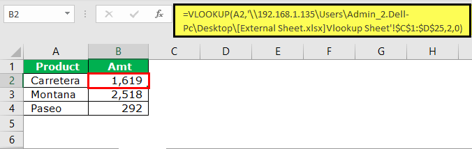
‘C:UsersAdmin_2.Dell-PCDesktop: This is the path to that sheet on the computer.

[External Sheet.xlsx]: This is the “Workbook” name in that path.

Vlookup Sheet: This is the “Worksheet” name in that workbook.

$C$1:$D$25: This is the range in that sheet.

What are External Links in Excel?
- Types of External Links in Excel
  - #1- Links within the Same Worksheet
  - #2 – Links from different worksheet but within the same workbook
  - #3 – Links from a different workbook
- How to Find, Edit, and Remove External Links in Excel?
  - Method #1: Using the Find & Replace Method with Operator Symbol
  - Method #2: Using the Find & Replace Method with File Extension
  - Method #3: Using Edit Link Option in Excel
- Things to Remember
- Recommended Articles

Types of External Links in Excel

Links within the same worksheet
Links from different worksheets but the same workbook
Links from a different workbook

You can download this External Links Excel Template here – External Links Excel Template

#1- Links within the Same Worksheet

These types of links are within the same worksheet. In a workbook, there are many sheets. This type of link specifies only the cell name.

For example, if we are in cell B2 and the formula bar reads A1, whatever happens in the A1 cell will reflect in cell B2.

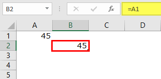
It is just a simple link within the same sheet.

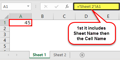
#2 – Links from different worksheets but within the same workbook

These types of links are within the same workbook but from different sheets.

For example, suppose there are two sheets in a workbook, and right now, we are in Sheet1 and giving a link from Sheet2.

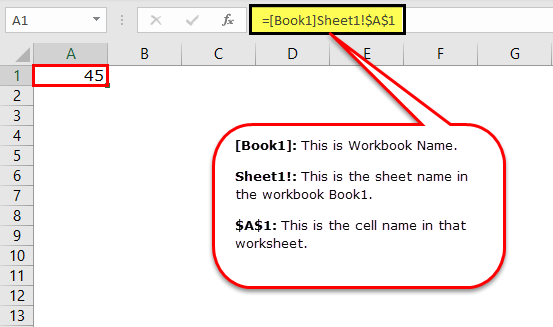
#3 – Links from a different workbook

This type of link is called an external link. It means this is altogether from a different workbook itself.

For example, if we give a link from another workbook called “Book1”, it will first show the workbook name, sheet name, and cell name.

How to Find, Edit, and Remove External Links in Excel?

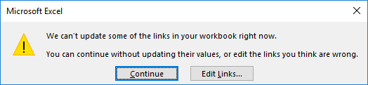
There are multiple ways we can find external links in the Excel workbook. As soon as we open a worksheet, we will get the below dialog box before we get inside the workbook, indicating that this workbook has external links.

Let us explain the methods to find external links in Excel.

Method #1: Using the Find & Replace Method with Operator Symbol

The link must have included its path or URL to the referring workbook if external links exist. The common in all the links is the operator symbol “[. “

Below are the steps to find external links using the “Find & Replace” method.

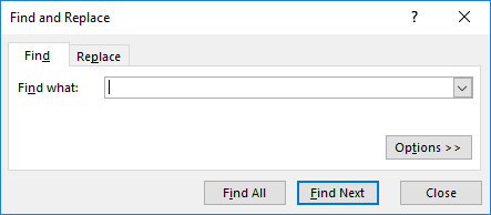
First, we must select the sheet and press the “Ctrl + F” keys (shortcut to find external links).
Then, we must insert the symbol “[” and click on “Find All.”

Method #2: Using the Find & Replace Method with File Extension

A cell with external references includes a workbook name and the workbook type.

The common file extensions are .xlsx , .xls , .xlsm , .xlb.

Step 1: First, we must select the sheet and press the “Ctrl + F” (shortcut to find external links).

Step 2: Now, we must insert “.xlsx” and click on “Find All.”

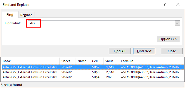
It will show all the external link cells.

Method #3: Using the Edit Link Option in Excel

It is the most direct option we have in Excel. It will highlight only the external link, unlike methods 1 and 2. We can edit the link in Excel, break, or delete and remove external links in this method.

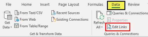
The “Edit Links” option in Excel is available under the “Data” tab.

method

Step 1: We must first select the cells we want to edit, break, or delete the link cells.

Step 2: Now, click on “Edit Links” in Excel. There are several options available here.

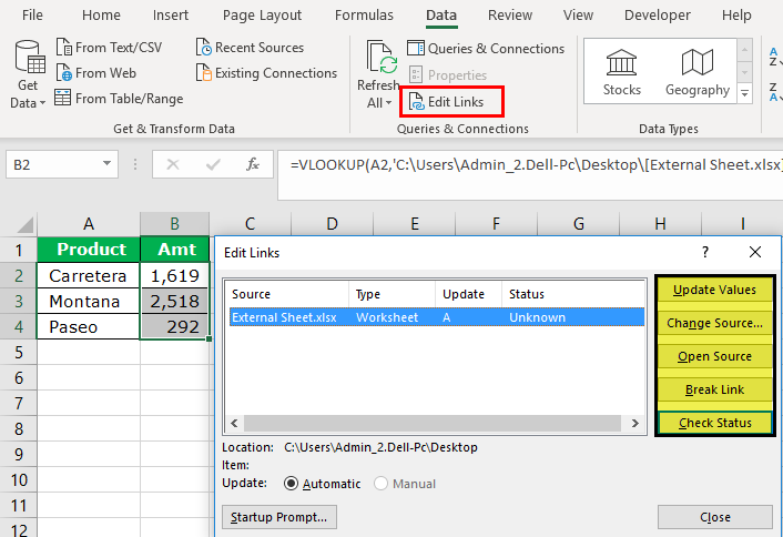
Update Values: This will update any changed values from the linked sheet.
Change Source: This will change the source file.
Open Source: This will open the source file instantly.
Break Link: This will permanently delete the formula, remove the external link, and retain only the values. Once this is done, we cannot undo it.
Check Status: This will check the status of the link.

Note: Sometimes, even if there is an external source, these methods would not show anything, but we must manually check graphs, charts, name ranges, data validation, condition formattingConditional formatting is a technique in Excel that allows us to format cells in a worksheet based on certain conditions. It can be found in the styles section of the Home tab.read more, chart title, shapes, or objects.

Things to Remember

We can find external links by using the VBA codeVBA code refers to a set of instructions written by the user in the Visual Basic Applications programming language on a Visual Basic Editor (VBE) to perform a specific task.read more. We must search on the internet to explore this.
If the external link is given to shapes, we must look for it manually.
The external formula links will not show the results in the case of SUMIF Formulas in ExcelThe SUMIF Excel function calculates the sum of a range of cells based on given criteria. The criteria can include dates, numbers, and text. For example, the formula “=SUMIF(B1:B5, “<=12”)” adds the values in the cell range B1:B5, which are less than or equal to 12.
read more, SUMIFS & COUNTIF formulasThe COUNTIF function in Excel counts the number of cells within a range based on pre-defined criteria. It is used to count cells that include dates, numbers, or text. For example, COUNTIF(A1:A10,”Trump”) will count the number of cells within the range A1:A10 that contain the text “Trump”
read more. It will show the values only if the sourced file is opened.
If Excel still shows an external link promptly, we must manually check all the formatting, charts, validation, etc.
Keeping external links can be helpful in case of auto-updating from the other sheet.

How To Edit Links In Excel?

Why can’t I edit links in Excel?

How do I find and edit links in Excel?

Find External Links using Edit Links Option

Go to the Data Tab.
In the Connections group, click on Edit Links. It opens the Edit Links dialog box will list all the workbooks that are being referenced.
Click on Break Links to convert all linked cells to values.

What is the fastest way to edit hyperlinks in Excel?

How do I edit a link?

Change an existing hyperlink

Right-click anywhere on the link and, on the shortcut menu, click Edit Hyperlink.
In the Edit Hyperlink dialog, select the text in the Text to display box.
Type the text you want to use for the link, and then click OK.

How do I remove links in Excel?

To remove multiple hyperlinks from an Excel spreadsheet, hold the Ctrl key and select the cells. Then you can select all the cells that include the links and click the Remove Hyperlink option.

How do I break links in Excel and keep values?

The Edit Links dialog box. Select the links in the dialog box. Click Break Links and acknowledge that you really want to break the selected links. Click OK.
Follow these steps:

Select the cells that contain links.
Press Ctrl+C.
Display the Paste Special dialog box.
Click the Values radio button.
Click OK.

How do I find the links in Excel?

Find links used in formulas

Press Ctrl+F to launch the Find and Replace dialog.
Click Options.
In the Find what box, enter .
In the Within box, click Workbook.
In the Look in box, click Formulas.
Click Find All.
In the list box that is displayed, look in the Formula column for formulas that contain .

How do I find links between sheets in Excel?

Finding Links to other Workbooks

Use Ctrl+F to display the Find dialog (Figure 1)
Type a [ in the Find what box.
Click the Options Why can’t I add a link in Excel?

How do I change a link in Excel?

In Excel 2010 and later:

Select all cells that contain hyperlinks, or press Ctrl+A to select all cells.
Right-click, and then click Remove Hyperlinks.

How do I change the text link in Excel?

Click the cell with the hyperlink.
Right-click the hyperlink style and select modify.
Click format in the style box.
Click font and choose what you want.
Click OK to close the box.

How do I shorten a link and rename it?

You can shorten a URL by using an URL shortener website, which will shrink your URL for free.
Here’s how to shorten a URL.

Copy the URL you want to shorten.
Open Bitly in your web browser.
Paste the URL into the “Shorten your link” field and click “Shorten.”
Click “Copy” to grab the new URL.

How do you shorten a URL?

For a Website

Copy the URL that you want to shorten.
Go to tinyurl.com.
Paste the long URL and click the “Make TinyURL!” button.
The shortened URL will appear. You can now copy and paste it where you need it.

How do I remove a link update in Excel?

Select File > Options > Advanced. Under General, click to clear the Ask to update automatic links check box.

How do you remove links in Excel without changing value?

Break a link

On the Data tab, in the Connections group, click Edit Links. Note: The Edit Links command is unavailable if your file does not contain linked information.
In the Source list, click the link that you want to break.
Click Break Link.

How do I open a link in Excel with keyboard?

How do I get Excel 2013 to automatically update links?

How do you tell if a spreadsheet is linked to another?

4 Answers

Go to Data Tab.
Choose Connections, this will open the Workbook Connections dialog.
In Workbook Connections dialog box it will list all of your connections.
Select the Connection in question and then click in the area below to see where it’s used.

Why do links break in Excel?

Источник

Break a link to an external reference in Excel

When you break a link to the source workbook of an external reference, all formulas that use the value in the source workbook are converted to their current values. For example, if you break the link to the external reference =SUM([Budget.xls]Annual!C10:C25), the SUM formula is replaced by the calculated value—whatever that may be. Also, because this action cannot be undone, you may want to save a version of the destination workbook as a backup.

If you use an external data range, a parameter in the query may be using data from another workbook. You may want to check for and remove any of these type of links.

Break a link

On the Data tab, in the Connections group, click Edit Links.

Note: The Edit Links command is unavailable if your file does not contain linked information.

In the Source list, click the link that you want to break.

To select multiple linked objects, hold down the CTRL key, and click each linked object.

To select all links, press Ctrl+A.

Click Break Link.

Delete the name of a defined link

If the link used a defined name, the name is not automatically removed. You may want to delete the name as well, by following these steps:

On the Formulas tab, in the Defined Names group, click Name Manager.

In the Name Manager dialog box, click the name that you want to change.

Click the name to select it.

Need more help?

You can always ask an expert in the Excel Tech Community or get support in the Answers community.

Источник

How to Find External Links or References in Excel

Manually finding external links or references in a spreadsheet is a cumbersome task. Microsoft does not have any inbuilt function that can find external references or links but still there do exist some workarounds to do this. And this is what I am going to share with you today.

Table of Contents

Method 1: Finding external References by using the find function

Though this is not a foolproof method still it can reduce the manual effort drastically. The main logic behind this method is that excel always encloses external references in long brackets “[]”. So, if you find all the “[]” brackets, you can easily get the list of external references used.

Open the excel sheet, for which you want to find the external references.
After this press the “Ctrl+F” keys to open the ‘Find’ and replace the dialog box.
In the find, textbox enter the string “[*]” (without quotes). This string means that resultant will be any string enclosed within long brackets.

Next, in the ‘Look in’ dropdown select Formulas and hit the “Find All” button.
The resultant will be a set of external references that are used in the sheet.

Method 2: Edit Links Option

On the excel ribbon there a ‘Data’ tab, inside this tab, there is an option called “Edit Links”.

Basically, the edit link option displays all the other files to which your spreadsheet is linked to. Please note that this option will be disabled by default and will only become active if your sheet contains some external references.

So, this can become a quick check to verify if your excel sheet contains external references or not. Using “Edit Links” is quite easy just follow the below steps to remove external references from your excel sheet:

Open your excel sheet and navigate to the ‘Data’ tab, select the option “Edit Links”.
In the “Edit Links” window all the spreadsheets which are referenced in your excel file will be listed.
On the right side of this Edit Links window there are options like ‘Update values (can be used for reloading the values)’, ‘Change Source (can be used to change the referenced file)’, ‘Open Source (opens the referenced excel files)’ and ‘Break Links (can be used to break the referenced links)’.

Among all these options ‘Break Links’ option is the one that we will be using, it breaks the references and replaces them with their current values.
Please note that the use of this feature should be done with utmost care as this cannot be undone.

Method 3: Find External Reference links by using Excel Macro

Using excel macros can be really helpful in finding the external reference links. To create a macro that can find and list down all the external links in a spreadsheet, follow the below steps:

With the excel sheet opened, navigate to the ‘View’ Tab, click on the ‘Macros’ button.

Now enter the macro name say “Fetch_Links” (without quotes) and hit the create button.
This will open the Excel VBA editor, simply paste the below code after the first line.

The whole code should look the same as shown in the below screenshot.

Now simply press the ‘F5’ button to run the macro. The code will create a new worksheet that contains all the external referenced links.

Method 4: Find and Delete Links Add-in

If you don’t want to use any of the first 3 methods then you should probably go for this one. Microsoft has now developed an Excel add-in that can run as a wizard and finds all the external links that your spreadsheet contains. It also has a feature to delete the referenced links.

You can find this add-in here.

Subscribe and be a part of our 15,000+ member family!

Now subscribe to Excel Trick and get a free copy of our ebook «200+ Excel Shortcuts» (printable format) to catapult your productivity.

Источник

Невозможно разорвать связи с другой книгой

Прежде чем разобрать причины ошибки разрыва связей, не лишним будет разобраться что такое вообще связи в Excel и откуда они берутся. Если все это Вам известно — можете пропустить этот раздел 🙂

Что такое связи в Excel и как их создать
Иногда при работе с различными отчетами приходится создавать связи с другими книгами(отчетами). Чаще всего это используется в функциях вроде ВПР (VLOOKUP) для получения данных по критерию из таблицы, расположенной в другой книге. Так же это может быть и простая ссылка на ячейки другой книги. В итоге ссылки в таких ячейках выглядят следующим образом:
=ВПР( A2 ;'[Продажи 2018.xlsx]Отчет’!$A:$F;4;0)
или
='[Продажи 2018.xlsx]Отчет’!$A1

[Продажи 2018.xlsx] — обозначает книгу, в которой итоговое значение. Такие книги так же называют источниками
Отчет — имя листа в этой книге
$A:$F и $A1 — непосредственно ячейка или диапазон со значениями

Если закрыть книгу, на которую была создана такая ссылка, то ссылка сразу изменяется и принимает более «длинный» вид:
=ВПР( A2 ;’C:UsersДмитрийDesktop[Продажи 2018.xlsx]Отчет’!$A:$F;4;0)
=’C:UsersДмитрийDesktop[Продажи 2018.xlsx]Отчет’!$A1
Предположу, что большинство такими ссылками не удивишь. Такие ссылки так же принято называть связыванием книг. Поэтому как только создается такая ссылка на вкладке Данные (Data) в группе Запросы и подключения (Queries & Coonections) активируется кнопка Изменить связи (Edit Links) . Там же, как несложно догадаться, их можно изменить. В большинстве случаев ни использование связей, ни их изменение не доставляет особых проблем. Даже если в книге источники были изменены значения ячеек, то при открытии книги со связью эти изменения будут так же автоматом обновлены. Но если книгу-источник переместили или переименовали — при следующем открытии книги со ссылками на неё Excel покажет сообщение о недоступных связях в книге и запрос на обновление этих ссылок:

Если нажать Продолжить , то ссылки обновлены не будут и в ячейках будут оставлены значения на момент последнего сохранения. Происходит это потому, что ссылки хранятся внутри самой книги и так же там хранятся значения этих ссылок. Если же нажать Изменить связи (Change Source) , то появится окно изменения связей, где можно будет выбрать каждую связь и указать правильное расположение нужного файла:

Так же изменение связей доступно непосредственно из вкладки Данные (Data)

Как разорвать связи
Как правило связи редко нужны на продолжительное время, т.к. они неизбежно увеличивают размер файла, особенно, если связей много. Поэтому чаще всего связь создается только для единовременно получения данных из другой книги. Исключениями являются случаи, когда связи делаются на общий файл, который ежедневного изменяется и дополняется различными сотрудниками и подразделениями, а в итоговом файле необходимо использовать именно актуальные данные этого файла.
Если решили разорвать связь, необходимо перейти на вкладку Данные (Data) -группа Запросы и подключения (Queries & Coonections) — Изменить связи (Edit Links) :

Выделить нужные связи и нажать Разорвать связь (Break Link) . При этом все ячейки с формулами, содержащими связи, будут преобразованы в значения вычисленные этой формулой при последнем обновлении. Данное действие нельзя будет отменить — только закрытием книги без сохранения.
Так же связи внутри формул разрываются, если формулы просто заменить значениями -выделяем нужные ячейки -копируем их -не снимая выделения жмем Правую кнопку мыши — Специальная вставка (Paste Special) — Значения (Values) . Формулы в ячейках будут заменены результатами их вычислений, а все связи будут удалены.
Более подробно про замену формул значениями можно узнать из статьи: Как удалить в ячейке формулу, оставив значения?

Что делать, если связи не разрываются

Но иногда возникают ситуации, когда вроде все формулы во всех ячейках уже заменены на значения, но запрос на обновление каких-то связей все равно появляется. В этом случае есть парочка рекомендаций для поиска и удаления этих мифических связей:

проверьте нет ли каких-либо связей в именованных диапазонах:
нажмите сочетание клавиш Ctrl + F3 или перейдите на вкладку Формулы (Formulas) —Диспетчер имен (Name Manager)
Читать подробнее про именованные диапазоны
Если в каком-либо имени есть ссылка с полным путем к какой-то книге(вроде такого ‘[Продажи 2018.xlsx]Отчет’!$A1 ), то такое имя надо либо изменить, либо удалить. Кстати, некоторые имена в итоге могут выдавать ошибку #ССЫЛКА! (#REF!) — к ним тоже стоит присмотреться. Имена с ошибками ничего хорошего как правило не делают.
Настоятельно рекомендую перед удалением имен создать резервную копию файла, т.к. неверное удаление таких имен может повлечь неправильную работу файла даже в случае, если сами ссылки возвращали в итоге ошибочное значение.
если удаление лишних имен не дает эффекта — проверьте условное форматирование:
вкладка Главная (Home) — Условное форматирование (Conditional formatting) — Управление правилами (Manage Rules) . В выпадающем списке проверить каждый лист и условия в нем:

Может случиться так, что условие было создано с использованием ссылки на другие книги. Как правило Excel запрещает это делать, но если ссылка будет внутри какого-то именованного диапазона — то диапазон такой можно будет применить в УФ, но после его удаления в самом УФ это имя все равно остается и генерирует ссылку на файл-источник. Такие условия можно удалять без сомнений — они все равно уже не выполняются как положено и лишь создают «пустую» связь.
Так же не помешает проверить наличие лишних ссылок и среди проверки данных(Что такое проверка данных). Как правило связи могут быть в проверке данных с типом Список. Но как их отыскать, если проверка данных распространена на множество ячеек?
Находим все ячейки с проверкой данных: выделяем одну любую ячейку на листе -вкладка Главная (Home) -группа Редактирование (Editing) — Найти и выделить (Find & Select) — Выделить группу ячеек (Go to Special) . Отмечаем Проверка данных (Data validation) — Всех (All) . Жмем Ок. После этого можно выделить все эти ячейки каким-либо цветом, чтобы удобнее было потом просматривать. Но такой метод выделит ВСЕ ячейки с проверками данных, а не только ошибочные.
Конечно, если вариантов кроме как найти руками нет и ячеек немного – просто заходим в проверку данных каждой ячейки(выделяем эту ячейку -вкладка Данные (Data) — Проверка данных (Data validation) ) и смотрим, есть ли там проблемная формула со ссылками на другие книги.
Можно поступить более кардинально – после того как выделили все ячейки с проверкой данных идем на вкладку Данные (Data) — Проверка данных (Data validation) и для всех ячеек в поле Тип данных (Allow) выбираем Любое значение (Any value) . Это удалит все формулы из проверки данных всех ячеек.
Но если ни удаление всех проверок данных, ни проверка каждой ячейки не подходит — я предлагаю коротенький код, который отыщет все такие ссылки быстрее и сэкономит время:

Option Explicit ‘————————————————————————————— ‘ Author : The_Prist(Щербаков Дмитрий) ‘ Профессиональная разработка приложений для MS Office любой сложности ‘ Проведение тренингов по MS Excel ‘ https://www.excel-vba.ru ‘ info@excel-vba.ru ‘ WebMoney — R298726502453; Яндекс.Деньги — 41001332272872 ‘ Purpose: ‘————————————————————————————— Sub FindErrLink() ‘надо посмотреть в Данные -Изменить связи ссылку на файл-иточник ‘и записать сюда ключевые слова в нижнем регистре(часть имени файла) ‘звездочка просто заменяет любое кол-во символов, чтобы не париться с точным названием Const sToFndLink$ = «*продажи 2018*» Dim rr As Range, rc As Range, rres As Range, s$ ‘определяем все ячейки с проверкой данных On Error Resume Next Set rr = ActiveSheet.UsedRange.SpecialCells(xlCellTypeAllValidation) If rr Is Nothing Then MsgBox «На активном листе нет ячеек с проверкой данных», vbInformation, «www.excel-vba.ru» Exit Sub End If On Error GoTo 0 ‘проверяем каждую ячейку на предмет наличия связей For Each rc In rr ‘на всякий случай пропускаем ошибки — такое тоже может быть ‘но наши связи должны быть без них и они точно отыщутся s = «» On Error Resume Next s = rc.Validation.Formula1 On Error GoTo 0 ‘нашли — собираем все в отдельный диапазон If LCase(s) Like sToFndLink Then If rres Is Nothing Then Set rres = rc Else Set rres = Union(rc, rres) End If End If Next ‘если связь есть — выделяем все ячейки с такими проверками данных If Not rres Is Nothing Then rres.Select ‘ rres.Interior.Color = vbRed ‘если надо выделить еще и цветом End If End Sub

Чтобы правильно использовать приведенный код, необходимо скопировать текст кода выше, перейти в редактор VBA( Alt + F11 ) -создать стандартный модуль(Insert —Module) и в него вставить скопированный текст. После чего вызвать макросы( Alt + F8 или вкладка Разработчик — Макросы ), выбрать FindErrLink и нажать выполнить.
Есть пара нюансов:

Прежде чем искать ненужную связь необходимо определить её ссылку: Данные (Data) -группа Запросы и подключения (Queries & Coonections) — Изменить связи (Edit Links) . Запомнить имя файла и записать в этой строке внутри кавычек:
Const sToFndLink$ = «*продажи 2018*»
Имя файла можно записать не полностью, все пробелы и другие символы можно заменить звездочкой дабы не ошибиться. Текст внутри кавычек должен быть в нижнем регистре. Например, на картинках выше есть связь с файлом «Продажи 2018.xlsx» , но я внутри кода записал «*продажи 2018*» — будет найдена любая связь, в имени которой есть «продажи 2018» .
Код ищет проверки данных только на активном листе
Код только выделяет все найденные ячейки(обычное выделение), он ничего сам не удаляет
Если надо подсветить ячейки цветом — достаточно убрать апостроф(‘) перед строкой
rres.Interior.Color = vbRed ‘если надо выделить еще и цветом

Как правило после описанных выше действий лишних связей остаться не должно. Но если вдруг связи остались и найти Вы их никак не можете или по каким-то причинам разорвать связи не получается(например, лист со связью защищен)- можно пойти совершенно иным путем. Действует этот рецепт только для файлов новых форматов Excel 2007 и выше (если проблема с файлом более старого формата — можно пересохранить в новый формат):

Обязательно делаем резервную копию файла, связи в котором никак не хотят разрываться
Открываем файл при помощи любого архиватора(WinRAR отлично справляется, но это может быть и другой, работающий с форматом ZIP)
В архиве перейти в папку xl ->externalLinks
Сколько связей содержится в файле, столько файлов вида externalLink1.xml и будет внутри. Файлы просто пронумерованы и никаких сведений о том, к какому конкретному файлу относится эта связь на поверхности нет. Чтобы узнать какой файл .xml к какой связи относится надо зайти в папку «_rels» и открыть там каждый из имеющихся файлов вида externalLink1.xml.rels . Там и будет содержаться имя файла-источника.
Если надо удалить только связь на конкретный файл — удаляем только те externalLink1.xml.rels и externalLink1.xml , которые относятся к нему. Если удалить надо все связи — удаляем все содержимое папки externalLinks
Закрываем архив
Открываем файл в Excel. Появится сообщение об ошибке вроде «Ошибка в части содержимого в Книге . «. Соглашаемся. Появится еще одно окно с перечислением ошибочного содержимого. Нажимаем закрыть.

После этого связи должны быть удалены.
Если и это не помогло — скорее всего «битая» связь связана с ошибкой самого файла и лучшим решением будет перенести все данные в новый файл.

Статья помогла? Поделись ссылкой с друзьями!

Источник

Перейти к содержанию

На чтение 2 мин Опубликовано 20.07.2015

Создание внешней ссылки
Оповещения
Редактирование ссылки

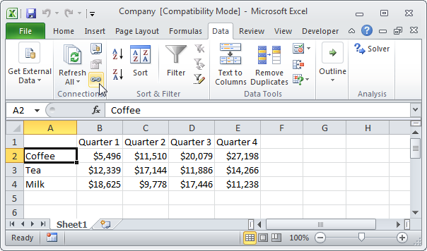
Внешняя ссылка в Excel – это ссылка на ячейку (или диапазон ячеек) в другой книге. На рисунках
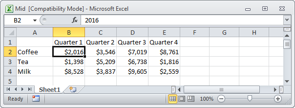
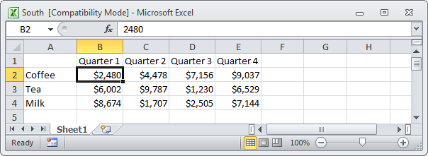
ниже вы видите книги из трех отделов (North, Mid и South).

Содержание

Создание внешней ссылки
Оповещения
Редактирование ссылки

Создание внешней ссылки

Чтобы создать внешнюю ссылку, следуйте инструкции ниже:

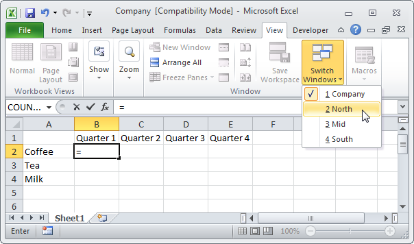
Откройте все три документа.
В книге «Company», выделите ячейку B2 и введите знак равенства «=».
На вкладке View (Вид) кликните по кнопке Switch Windows (Перейти в другое окно) и выберите «North».
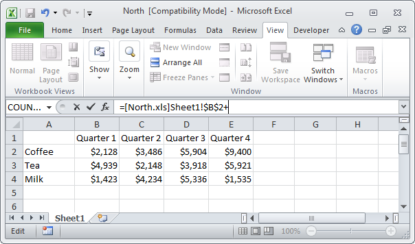
В книге «North», выделите ячейку B2 и введите «+».
Повторите шаги 3 и 4 для книг «Mid» и «South».
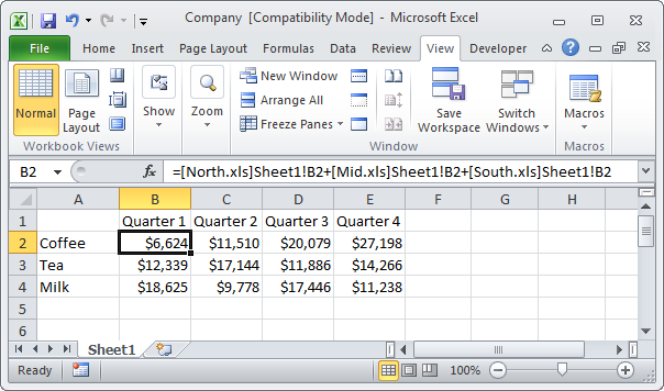
Уберите символы «$» в формуле ячейки B2 и скопируйте эту формулу в другие ячейки.Результат:

Оповещения

Закройте все документы. Внесите изменения в книги отделов. Снова закройте все документы. Откройте файл «Company».

Чтобы обновить все ссылки, кликните по кнопке Enable Content (Включить содержимое).
Чтобы ссылки не обновлялись, нажмите кнопку X.

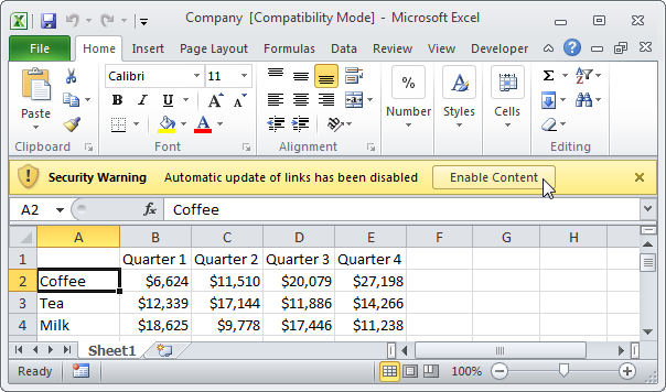
Примечание: Если вы видите другое оповещение, нажмите Update (Обновить) или Don’t Update (Не обновлять).

Редактирование ссылки

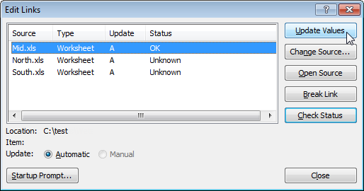
Чтобы открыть диалоговое окно Edit Links (Изменение связей), на вкладке Data (Данные) в разделе Connections group (Подключения) щелкните Edit links symbol (Изменить связи).

Если вы не обновили ссылки сразу, можете обновить их здесь. Выберите книгу и нажмите кнопку Update Values (Обновить), чтобы обновить ссылки на эту книгу. Обратите внимание, что Status (Статус) изменяется на ОК.
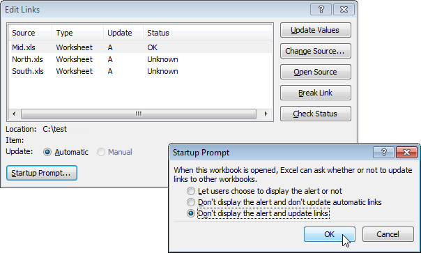
Если вы не хотите обновлять ссылки автоматически и не желаете, чтобы отображались уведомления, кликните по кнопке Startup Prompt (Запрос на обновление связей), выберите третий вариант и нажмите ОК.

Оцените качество статьи. Нам важно ваше мнение:

Источник

Need more help?

See Also

Why can’t I edit links in Excel?

How do I find and edit links in Excel?

How do you edit a shared link in Excel?

What is the fastest way to edit hyperlinks in Excel?

How do I edit a link?

How do I remove links in Excel?

How do I break links in Excel and keep values?

How do I find the links in Excel?

How do I find links between sheets in Excel?

Why can’t I add a link in Excel?

How do I change a link in Excel?

How do I change the text link in Excel?

How do I shorten a link and rename it?

How do you shorten a URL?

How do I remove a link update in Excel?

How do you remove links in Excel without changing value?

How do I open a link in Excel with keyboard?

How do I get Excel 2013 to automatically update links?

How do you tell if a spreadsheet is linked to another?

Why do links break in Excel?

What are External Links in Excel?

Table of contents

Types of External Links in Excel

#1- Links within the Same Worksheet

#2 – Links from different worksheets but within the same workbook

#3 – Links from a different workbook

How to Find, Edit, and Remove External Links in Excel?

Method #1: Using the Find & Replace Method with Operator Symbol

Method #2: Using the Find & Replace Method with File Extension

Method #3: Using the Edit Link Option in Excel

Things to Remember

Recommended Articles

How To Edit Links In Excel?

Why can’t I edit links in Excel?

How do I find and edit links in Excel?

What is the fastest way to edit hyperlinks in Excel?

How do I edit a link?

How do I remove links in Excel?

How do I break links in Excel and keep values?

How do I find the links in Excel?

How do I find links between sheets in Excel?

How do I change a link in Excel?

How do I change the text link in Excel?

How do I shorten a link and rename it?

How do you shorten a URL?

How do I remove a link update in Excel?

How do you remove links in Excel without changing value?

How do I open a link in Excel with keyboard?

How do I get Excel 2013 to automatically update links?

How do you tell if a spreadsheet is linked to another?

Why do links break in Excel?

Break a link to an external reference in Excel

Break a link

Delete the name of a defined link

Need more help?

How to Find External Links or References in Excel

Method 1: Finding external References by using the find function

Method 2: Edit Links Option

Method 3: Find External Reference links by using Excel Macro

Method 4: Find and Delete Links Add-in

Subscribe and be a part of our 15,000+ member family!

Невозможно разорвать связи с другой книгой

Создание внешней ссылки

Оповещения

Редактирование ссылки