
Modifying tables
- Select any cell in your table. The Design tab will appear on the Ribbon.
- From the Design tab, click the Resize Table command. Resize Table command.
- Directly on your spreadsheet, select the new range of cells you want your table to cover. You must select your original table cells as well.
- Click OK.
Contents
- 1 How do I edit text in an Excel table?
- 2 How do you add data to a table in Excel?
- 3 How do I edit cells in a table?
- 4 How do you edit cells in Excel without clicking?
- 5 Can’t edit anything in Excel?
- 6 How do I change a table range in Excel?
- 7 How would you add or remove cells in a table?
- 8 How do I change a table to grid table 4?
- 9 How do you make a table cell editable on button click?
- 10 How do I type in a table in pages?
- 11 How do I enter edit mode in Excel?
- 12 How do I make all Excel sheets editable?
- 13 Why is Excel locked for editing?
- 14 What is the shortcut key to edit a cell in Excel?
- 15 What is the shortcut to activate edit mode in Excel?
- 16 How do I fix a table in Excel?
- 17 Where is table tools in Excel?
- 18 How can you add and remove any column of a table?
- 19 How do you get Excel to add up a column?
- 20 How do you add cells in a table?
How do I edit text in an Excel table?
Click the cell that contains the data that you want to edit, and then click anywhere in the formula bar. This starts Edit mode and positions the cursor in the formula bar at the location that you clicked. Click the cell that contains the data that you want to edit, and then press F2.
How do you add data to a table in Excel?
The most direct way to add new data is to press the Tab key when the cell cursor is in the last cell of the last record (row). Doing this causes Excel to add another row to the table, where you can enter the appropriate information for the next record.
How do I edit cells in a table?
Select the cells you want to change. Right-click the table, and then click Format Table. In the Format Table dialog box, click the Cell Properties tab. Under Text Box Margins, enter the margins you want.
How do you edit cells in Excel without clicking?
You can press the F2 key to get into the editing mode of a cell without double clicking it. It is easy to operate, you just need to select the cell you want to edit and press the F2 key, and the cursor will be located at the end of the cell value, then you can edit the cell immediately.
Can’t edit anything in Excel?
a. Select File > Options > Select Advanced from the Excel menu bar. b. On Editing options, ensure that the check box Allow editing directly in cells is checked.
How do I change a table range in Excel?
Convert an Excel table to a range of data
- Click anywhere in the table and then go to Table Tools > Design on the Ribbon.
- In the Tools group, click Convert to Range. -OR- Right-click the table, then in the shortcut menu, click Table > Convert to Range.
How would you add or remove cells in a table?
Under Table Tools, on the Layout tab, in the Rows & Columns group, do one of the following:
- To add a row above the selected cell, click Insert Above.
- To add a row below the selected cell, click Insert Below. Notes: To add a row at the end of a table, you can click the rightmost cell of the last row, and then press TAB.
How do I change a table to grid table 4?
Navigate to the Insert tab, then click the Table command. This will open a drop-down menu that contains a grid. Hover over the grid to select the number of columns and rows you want. Click the grid to confirm your selection, and a table will appear.
How do you make a table cell editable on button click?
Make table cells editable on click. On click – the cell should become “editable” (textarea appears inside), we can change HTML. There should be no resize, all geometry should remain the same. Buttons OK and CANCEL appear below the cell to finish/cancel the editing.
How do I type in a table in pages?
Add or delete a table in Pages on Mac
- Do one of the following: Place the table within the text: Click in the text where you want the table to appear.
- Click. in the toolbar, then select a table or drag one to the page.
- Do any of the following: Type in a cell: Click the cell, then start typing.
How do I enter edit mode in Excel?
Click the cell you want to edit. Use the mouse to click the formula bar at the top of the window. The cell activates, and it switches to editing mode. You can also double-click the cell to activate editing mode, or you can press the “F2” key.
How do I make all Excel sheets editable?
On the Tools menu, click Share Workbook, and then click the Editing tab. Click to select the Allow changes by more than one user at the same time check box, and then click OK. Save the workbook when you are prompted.
Why is Excel locked for editing?
If you have locked the file yourself, it might be because the file is open on a different device, or the previous instance of the file didn’t close properly. Tip: Sometimes a file may get locked if everyone editing isn’t using a version that supports co-authoring.
What is the shortcut key to edit a cell in Excel?
F2
First, the keyboard shortcut for editing a cell is F2 on Windows, and Control + U on a Mac. With Excel’s default settings, this will put your cursor directly in the cell, ready to edit.
What is the shortcut to activate edit mode in Excel?
To do this, you must first press the F2 key on your desired cell to activate “Edit” mode (see our prior keyboard shortcut on the Double F2 key). Once you are in “Edit” mode, you have the flexibility to highlight any part of your formula to evaluate it, so long as it could have been evaluated as a stand-alone formula.
How do I fix a table in Excel?
How to freeze a row in Excel
- Select the row right below the row or rows you want to freeze.
- Go to the View tab.
- Select the Freeze Panes option and click “Freeze Panes.” This selection can be found in the same place where “New Window” and “Arrange All” are located.
Where is table tools in Excel?
The Table Tools add-in was designed to make your life with tables easier. It installs a TOOLS ribbon tab right next to the DESIGN ribbon tab when you select a table cell. * In it you’ll find functionality previously either difficult or non-existent in Excel.
How can you add and remove any column of a table?
The statement ALTER TABLE is mainly used to delete, add, or modify the columns into an existing table.
Syntax of ADD COLUMN
- ALTER TABLE table_name (Name of the table)
- ADD [COLUMN] column_definition, (for adding column)
- ADD [COLUMN] column_definition,
- …;
How do you get Excel to add up a column?
If you need to sum a column or row of numbers, let Excel do the math for you. Select a cell next to the numbers you want to sum, click AutoSum on the Home tab, press Enter, and you’re done. When you click AutoSum, Excel automatically enters a formula (that uses the SUM function) to sum the numbers.
How do you add cells in a table?
Inserting Cells in a Table
- Select the cell before which you want a cell inserted.
- Choose Insert Cells from the Table menu. You will see the Insert Cells dialog box.
- Select which way you want the cells to be adjusted.
- Click on OK.
![]()
Download Article
![]()
Download Article
After you create a pivot table, you might need to edit it later. This wikiHow will show you how to edit a pivot table in Excel on your computer by adding or changing the source data. After you make any changes to the data for your Pivot Table, you will need to refresh it to see any changes.
Steps
-

1
Open your project in Excel. To do this, double-click the Excel document that contains your pivot table in Finder (Macs) or File Explorer (Windows). Alternatively, if you already have Excel open, click File > Open and select the file that has your pivot table.
-
2
Go to the spreadsheet page that contains the data for the pivot table. Click the tab that contains your data (e.g., Sheet 2) at the bottom of the Excel window.
Advertisement
-
3
Add or change your data. Enter the data that you want to add to your pivot table directly next to or below the current data.
- For example, if you have data in cells A1 through E10, you would add another column in the F column or another row in the 11 row.
- If you simply want to change the data in your pivot table, edit the data here. It won’t be reflected in the pivot table until you refresh the data, though.
-
4
Go back to the pivot table tab. Click the tab on which your pivot table is listed.
-
5
Select your pivot table. Click the pivot table to select it.
-
6
Click the Analyze tab. It’s in the middle of the editing ribbon that’s at the top of the Excel window. Doing so will open a toolbar just below the editing ribbon.
- On a Mac, click the PivotTable Analyze tab here instead.
-
7
Click Change Data Source. This option is in the «Data» section of the Analyze toolbar. A drop-down menu will appear.
-
8
Click Change Data Source…. It’s in the drop-down menu. Doing so opens a window.
-
9
Select your data. Click and drag from the top-left cell in your data group down to the bottom-left cell in the group. This will include the column(s) or row(s) that you added.
-
10
Click OK. It’s at the bottom of the window.
-
11
Click Refresh. It’s in the «Data» section of the toolbar.
- If you added a new column to your pivot table, check its box on the right side of the Excel window to display it.[1]
- If you added a new column to your pivot table, check its box on the right side of the Excel window to display it.[1]


Advertisement
Ask a Question
200 characters left
Include your email address to get a message when this question is answered.
Submit
Advertisement
Thanks for submitting a tip for review!
References
About This Article
Article SummaryX
1. Open your project in Excel.
2. Go to the spreadsheet that contains the data for the pivot table
3. Add or change your data.
4. Go back to the pivot table tab.
5. Select your pivot table.
6. Click Analyze tab (Windows) or PivotTable Analyze (Mac).
7. Click Change Data Source.
8. Click Change Data Source.
9. Select your data.
10. Click Ok.
11. Click Refresh.
Did this summary help you?
Thanks to all authors for creating a page that has been read 50,233 times.
Is this article up to date?
Create and format tables
Create and format a table to visually group and analyze data.
Note: Excel tables shouldn’t be confused with the data tables that are part of a suite of What-If Analysis commands (Forecast, on the Data tab). See Introduction to What-If Analysis for more information.

Try it!
-
Select a cell within your data.
-
Select Home > Format as Table.
-
Choose a style for your table.
-
In the Create Table dialog box, set your cell range.
-
Mark if your table has headers.
-
Select OK.
-
Insert a table in your spreadsheet. See Overview of Excel tables for more information.
-
Select a cell within your data.
-
Select Home > Format as Table.
-
Choose a style for your table.
-
In the Create Table dialog box, set your cell range.
-
Mark if your table has headers.
-
Select OK.
To add a blank table, select the cells you want included in the table and click Insert > Table.
To format existing data as a table by using the default table style, do this:
-
Select the cells containing the data.
-
Click Home > Table > Format as Table.
-
If you don’t check the My table has headers box, Excel for the web adds headers with default names like Column1 and Column2 above the data. To rename a default header, double-click it and type a new name.
Note: You can’t change the default table formatting in Excel for the web.
Want more?
Overview of Excel tables
Video: Create and format an Excel table
Total the data in an Excel table
Format an Excel table
Resize a table by adding or removing rows and columns
Filter data in a range or table
Convert a table to a range
Using structured references with Excel tables
Excel table compatibility issues
Export an Excel table to SharePoint
Need more help?
Author: Oscar Cronquist Article last updated on February 07, 2023
An Excel Table is a very useful feature in Excel, it was introduced in Excel 2007. Earlier versions had this feature as well but it was then known as Excel Lists.
What can an Excel Table do for you? It will simplify your work with data, adding or removing data, filtering, totals, sorting, enhance readability using cell formatting, cell references, formulas, and more. I will go through all this in greater detail, keep on reading.
Table of Contents
- How to create an Excel Table
- How to name an Excel Table
- How to manipulate Excel Table data
- How to edit an Excel Table value
- How to delete an Excel Table value
- How to add a row
- How to add a column
- How to delete an Excel Table row
- How to delete an Excel Table column
- How to delete an Excel Table and keep values
- How to sort an Excel Table
- How to filter an Excel Table
- How to insert a total to an Excel Table and sum using a condition
- How do structured references work?
- Reference an entire Excel Table
- Reference Excel Table data
- Reference column headers
- Reference a column
- Reference a value on the same row
- How to use a formula in an Excel Table
- How to change Excel Table formatting
- How to show Excel Table totals
- List all tables in a workbook — Named ranges
- How to link a chart to an Excel Table
- How to link a drop-down list to an Excel Table (Data validation)
- Working with filtered Excel Tables
- How to quickly find an Excel Table in a workbook
- Count unique distinct values in a filtered Excel Table (Link)
- Extract unique distinct values from a filtered Excel Table (Link)
- Filter duplicate records [Excel Table] (Link)
1. How to create an Excel Table
Follow these simple steps to convert a cell range to a table:
- Go to tab «Insert» on the ribbon
- Select your data set
- Press with left mouse button on the «Table» button on tab «Insert»
- Press with left mouse button on the «OK» button if your table has headers, if not deselect the check box and press with left mouse button on «OK». Excel will automatically create headers for you.
- You have built an excel table
Tip! Use short cut keys CTRL + T to quickly build a table.
Back to top
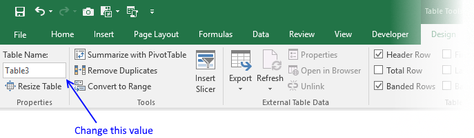
2. How to name an Excel Table
I recommend you give the table and table headers descriptive names, for example, it will be easier to identify cell references to Excel Tables in formulas. Cell references are called structured references and you can read about these in this article as well.
- Select a cell in your table
- Excel automatically navigates to tab «Design» on your ribbon
- Change table name
- Press Enter
Back to top
3. How to manipulate Excel Table data
3.1 How to edit an Excel Table value
- Doublepress with left mouse button on any cell with left mouse button to start editing an Excel Table value.
- Use arrow keys to move the prompt between characters.
- Press Enter to apply changes or press CTRL + SHIFT + Enter to create an array formula.
3.2 How to delete an Excel Table value
- Press with left mouse button on with the left mouse button on any cell in the Excel Table to select it.
- Press Delete on the keyboard to remove the cell value.
3.3 How to add a row
- Press with left mouse button on with the left mouse button on any cell in the Excel Table to select it.
- Press the Tab key repeatedly until a new row is created.
A new row is created if you press the tab key with the lower right cell in the Excel Table selected. See the animated picture above.
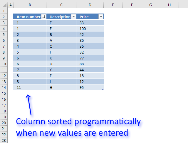
Here is another way to create a new row.
- Select any cell right below the Excel Table the cell must be adjacent to the Excel Table for this to work.
- Type a value or a formula.
- Press Enter.
The Excel Table grows automatically when you add values adjacent to the Excel Table.
3.4 How to add a column
- Press with mouse on any cell adjacent to the Excel Table with the left mouse button to select it.
- Type a value or formula.
- Press Enter or CTRL + SHIFT + Enter.
The table expands automatically when you add values to adjacent cells, see the animated image above.
Add data to a cell adjacent to the table and the table expands automatically.
3.5 How to delete an Excel Table row
- Press with right mouse button on on one of the cells on the row you want to delete in the Excel Table.
- A popup menu appears, press with left mouse button on «Delete» on the popup menu.
- Another popup menu shows up, press with left mouse button on Table Rows.
This deletes the entire Excel Table row, it does not delete other values outside the Excel Table. At least not in Excel 365.
3.6 How to delete an Excel Table column
- Press with right mouse button on on any cell in an Excel Table. A popup menu appears.
- Press with mouse on «Delete» on the popup menu. Another popup menu shows up.
- Press with mouse on «Table Columns» .
3.7 How to delete an Excel Table and keep values

- Press with mouse on any cell in the Excel Table to select it. A tab named «Table Design» appears on the ribbon, this tab is not visible if not a cell in the Excel Table is sleected.
- Press with mouse on tab «Table Design» on the ribbon.
- Press with mouse on the «Convert to Range» button, see the image above.

The image above shows the Excel Table after converting to a normal range of cells. However, the cell formatting is still preserved.
Here is how to remove the cell formatting as well:
- Select the entire data set.
- Go to tab «Home» on the ribbon.
- Press with mouse on «Clear» button. A popup menu appears.
- Press with left mouse button on «Clear Formats».

Back to top
4. How to sort an Excel Table
Sorting a table is easy, press with left mouse button on any black triangle located at each header, a menu appears allowing you to quickly sort data in a descending or ascending order.
An arrow next to the black triangle indicates sort order. Sort Z to A (descending) shows you an arrow pointing down.
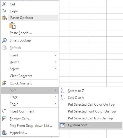
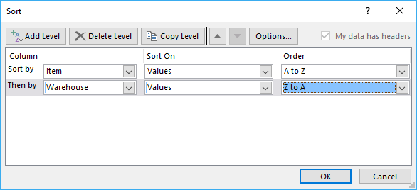
You can also sort on multiple columns, follow these steps.
- Press with right mouse button on on a cell
- Press with left mouse button on Sort and then press with left mouse button on «Custom Sort…»

- Select column name to sort on and sort order then add more columns.

- Press with left mouse button on OK button to apply sort settings to table
The following article demonstartes how to sort a values in an excel defined table using a macro:
Recommended articles
Back to top
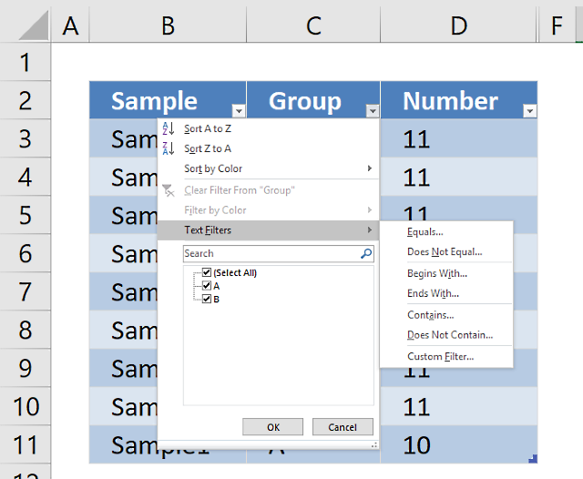
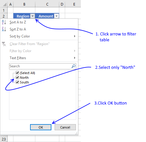
5. How to filter an Excel Table
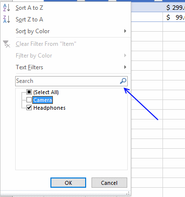
- Press with mouse on a black triangle next to any header
- Select values you want to filter
- Press with left mouse button on OK button
See animated picture below.
Excel allows you to apply filters to multiple columns easily, repeat above steps with another column.
Use the search field to quickly find the value you want to filter, see picture below.
Back to top
6. How to insert a total to an Excel Table and sum using a condition
You can quickly sum values using table filtering.
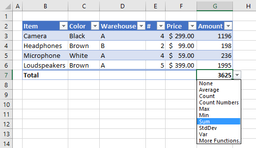
Select a cell in the table, then go to tab «Design» on the ribbon.
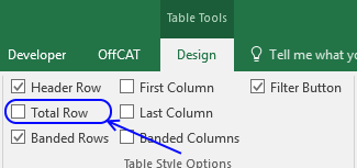
Press with left mouse button on «Checkbox» to enable «Total Row».
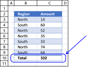
A row with totals appears on your table (332), see picture above.
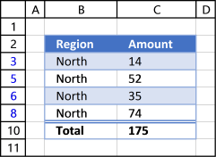
Now filter the table, see instructions on picture below.
See how the total changes from 332 to 175.
Back to top
7. How do structured references work?
You are probably used to cell references like this one:
=SUM(E3:E6)
Creating a cell reference to a table column returns this instead, see picture below.
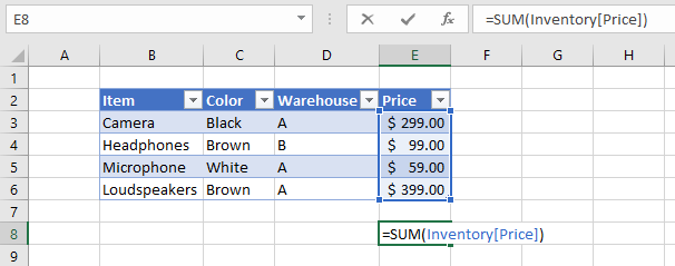
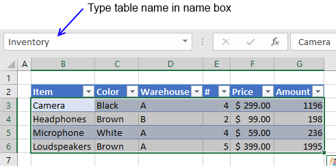
First the table name (Inventory) and then the column name enclosed with brackets [Price].
What is the purpose of structured references? The amazing thing with structured references is that if you add or remove values to a table the structured reference stays the same, no need to update cell references. In other words, they are dynamic.
7.1 Reference an entire Excel Table

The following structured reference returns the entire Excel Table including the column header names.
Formula in cell B9:
=Table1[#All]
Back to top
7.2 Reference Excel Table data

The following structured reference returns all Excel Table data, however, no the column header names.
Formula in cell B9:
=Table1
Back to top
7.3 Reference all column headers

The following structured reference returns all Excel Table column header names.
Formula in cell B9:
=Table1[#Headers]
Back to top
7.4 Reference a column

The following structured reference returns all Excel Table data from a given column.
Formula in cell B9:
=Table1[East]
Back to top

The following structured reference returns all Excel Table data from a given column including the column header name.
Formula in cell B9:
=Table1[[#All],[East]]
Back to top
7.5 Reference a value on the same row

The following structured reference returns an Excel Table value from a given column but on the same row as the formula is entered on.
Formula in cell G4:
=Table1[@North]
Back to top
8. How to use a formula in an Excel Table
The following example demonstrates what happens if I type a formula in an excel table. I want to multiply cell E3 with F3 in cell G3, see animated picture below.
Excel creates these structured cell references in cell G3 if I type = (equal sig) and then press with left mouse button on cell E3, type * (asterisk) and then press with left mouse button on cell F3:
=[@[‘#]]*[@Price]
@ (at) means cell value on same row as formula.
Excel also calculates the remaining cells in column G automatically, see animated picture above.
Creating a reference to the entire excel table and headers returns this: =Inventory[#All]
A reference to data in table looks like this: =Inventory
A reference to a table column returns: =Inventory[Warehouse]
A reference to a column header only looks like this: =Inventory[[#Headers],[Warehouse]]
Back to top
9. How to change Excel Table formatting
- Select a cell in excel table
- Go to tab «Design» on the ribbon

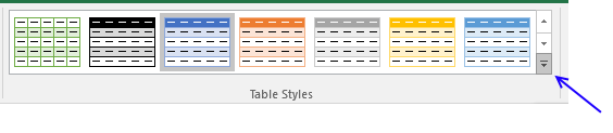
- Hover over a table style and see your table change

- If you like it press with left mouse button on it to select it
- Press with left mouse button on the black triangle to se even more table styles

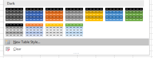
You can also build your own table style.
- Select a table cell
- Go to tab «Design»
- Press with left mouse button on black triangle
- Press with left mouse button on «New Table Style…»

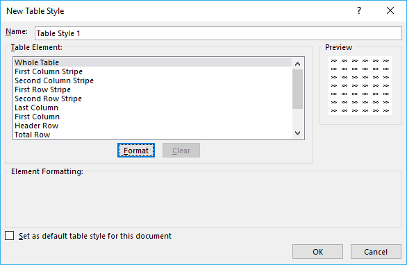
- Enter a name for your table style

- Select a table element you want to change
- Press with left mouse button on «Format» button

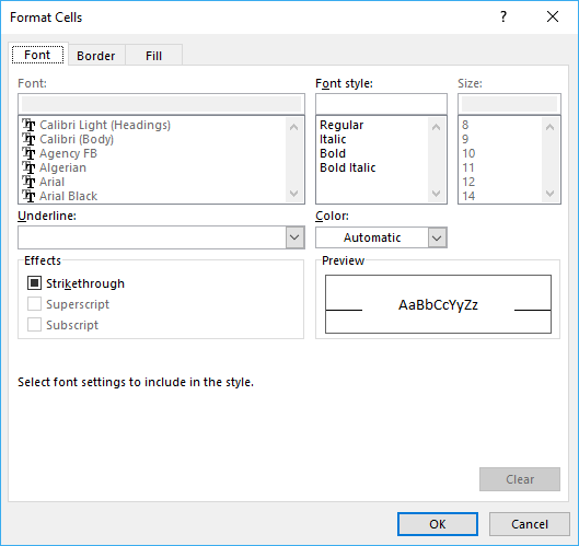
- Format as you like
- Press with left mouse button on OK button twice
Back to top
10. How to show Excel Table totals
- Press with mouse on a cell in an excel table
- Go to tab «Design»

- Press with left mouse button on «Total Row» check box

- Press with left mouse button on cell G7 and then on black triangle

- You can change how value in cell G7 is calculated, the menu has these formulas: Average, Count, Count Numbers, Max, Min, Sum, StdDev, Var and More Functions.
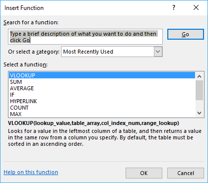
- If you press with left mouse button on «More Functions» a dialog box opens with formulas to choose from.

Back to top
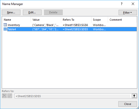
11. List all tables in workbook — Named ranges
The Name Manager contains a list of all named ranges and Excel tables in your workbook.
- Press with left mouse button on the «Formula» tab on the ribbon.
- Press with left mouse button on «Name Manager» button.

There are only Excel Tables in this workbook so the dialog box shows the Excel Table names, there are no named ranges in this workbook. See the image above.
Back to top
12. How to link a chart to an Excel Table
Combine chart and table to make use of dynamic cell references while filtering data.
More details here: How to create a dynamic chart
Back to top
13. How to link a drop-down list to an Excel Table (Data validation)
The following animation shows you a data validation list linked to a table.
Read this post if you are interested in the details:
How to use a table name in data validation lists and conditional formatting formulas
Back to top
14. Working with a filtered Excel Table
If you try to use a filtered table as a data source in a formula you are in for trouble, see animated picture below.
As you can see above the SUM function sums all values in table regardless of filtered or not.
I have written a few articles about this:
- Highlight duplicates in a filtered excel defined table
- Count unique distinct values in a filtered table
- Highlight unique values in a filtered excel table
- Populate a list box with visible unique values from an excel table (vba)
- Highlight unique values in a filtered excel table
- Extract unique distinct values from a filtered table (udf and array formula)
- Vlookup visible data in a table and return multiple values
Back to top
15. How to quickly find an Excel Table in a workbook
Excel lets you quickly focus on a table if you type the table name in the name box.
Back to top
What are Excel Tables?
Tables in Excel helps group related data into one or more rows and/or columns. Once a table is created, Excel assigns a unique name to the columns and the table itself. Such names are used as structured references, which make it easy to apply Excel formulas. Therefore, tables eliminate the need to create named ranges in Excel.
For example, the following image shows a usual data range on the left side and an Excel table on the right side. Notice the alternately colored excel rowsThe two different methods to add colour to alternative rows are adding alternative row colour using Excel table styles or highlighting alternative rows using the Excel conditional formatting option.read more and structured references (in cell J2) of the latter.
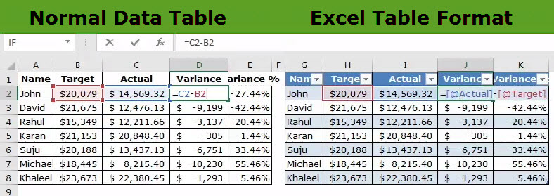
The purpose of creating tables is to make the data manageable, organized, and fit for analysis. Apart from structured references, tables offer several benefits like quick sorting and filtering, automatic expansion, easy formatting, readable formulas, and so on. Tables are extremely helpful when working with large databases.
Table of contents
- What are Excel Tables?
- How to Create Tables in Excel?
- How to Customize Tables in Excel?
- #1–Change the Name of the Table
- #2–Change the Color of the Table
- What are the Advantages of Creating Tables in Excel?
- #1–Creates Structured References Automatically
- #2–Is Dynamic in Nature
- #3–Makes it Easy to Work With PivotTables
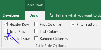
- #4–Freezes Header Row Automatically
- #5–Helps add a Total Row Containing Functions
- #6–Eases Restoring to Usual Data Range Without Losing the Table Style
- #7–Helps add Slicers for Filtering Data
- #8–Assists in Creating Reports in Power BI
- How to Turn off Structured References in Excel?
- Frequently Asked Questions
- Recommended Articles
How to Create Tables in Excel?
You can download this Excel Tables Template here – Excel Tables Template
The steps to create a table in Excel are listed as follows:
- Ensure that the raw data does not contain any empty rows and/or columns. Further, each column should have a unique heading. If any two columns have the same headers, Excel automatically changes one of these headers once a table is created.
The raw data is shown in the following image.
Note: A column header should not contain any Excel formulas.

- Select any cell of the raw data and press the shortcut “Ctrl+T.” Both keys of the shortcut should be pressed together.
Note: Alternatively, after selecting a cell of the raw data, click “table” from the Insert tab of Excel. This option is in the “tables” group of the Excel ribbon.

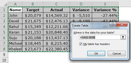
- The “create table” dialog box opens, as shown in the following image. Excel automatically selects the range for the table. Check whether this range is correct or not. If not, it can be edited.

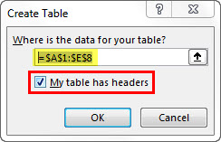
- Select or deselect the checkbox of “my table has headers.” If selected, Excel will treat the content of the first row (row 1) as column headers.
In the preceding table, row 1 does contain column headers. So, we have selected the option “my table has headers.” Next, click “Ok.”

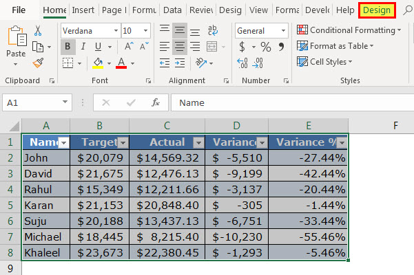
- An Excel table has been created. It is shown in the following image. Notice that the banded rows and filters (to the right of each column header) appear automatically.
Note: In Excel, banded rows are those in which color or shading is applied alternately.


How to Customize Tables in Excel?
A table can be customized by changing its name and/or the default color (or table style). Let us learn how this is done.
#1–Change the Name of the Table
When a table is created, Excel assigns a default name like “table1,” “table2,” etc., depending on whether it is the first or the second table of the current workbook.
Working with such default names may become confusing, especially when there are lots of tables. So, the solution is to assign unique names to each table.
The steps for changing the name of the Excel table are listed as follows:
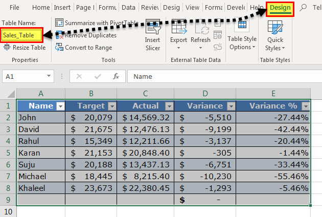
Step 1: Select the entire table. Once selected, the Design tab appears on the Excel ribbonRibbons in Excel 2016 are designed to help you easily locate the command you want to use. Ribbons are organized into logical groups called Tabs, each of which has its own set of functions.read more. This tab is shown within a red box in the following image.
Note: In place of the entire table, even if a single cell is selected, the Design tab will become visible.
Step 2: In the Design tab, perform the following tasks:
- Click inside the box under “table name.” This box is displayed in the “properties” group at the leftmost side of the ribbon.
- Enter the desired name in this box.
- Press the “Enter” key.
Our table has been named “Sales_Table.” This is shown in the following image.
Rules Governing the Table Names
While naming a table, the following points should be considered:
- The name should always begin with a letter, a backslash () or an underscore (_).
- The name cannot be the single letter “r” (or “R”) or “c” (or “C”).
- The name should not consist of any spaces. Instead, one can use an underscore (_) or a period (.) to separate the words.
- The name can contain numbers, but cell references should be avoided.
- The name can contain a maximum of 255 characters.
- The name of the table should be unique. In case of a duplicate name, a message will be displayed saying that a unique name should be chosen.
Note: A name is said to be duplicate if two tables within the same workbook have the same names. Further, Excel does not distinguish between the uppercase and lowercase letters in the name of a table. So, the names “abc” or “ABC” are considered the same by Excel.
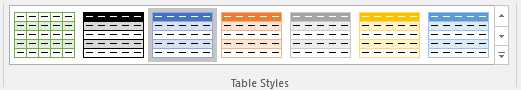
#2–Change the Color of the Table
When a table is created, Excel assigns it a default color. To change the color of the table, its style needs to be changed. Excel displays a list of different table styles from which one can choose the desired option.
The steps to change the color (or style) of a table are listed as follows:
Step 1: Select either a cell of the table or the entire table. We have selected the latter. The Design tab becomes visible, as shown in the following image.

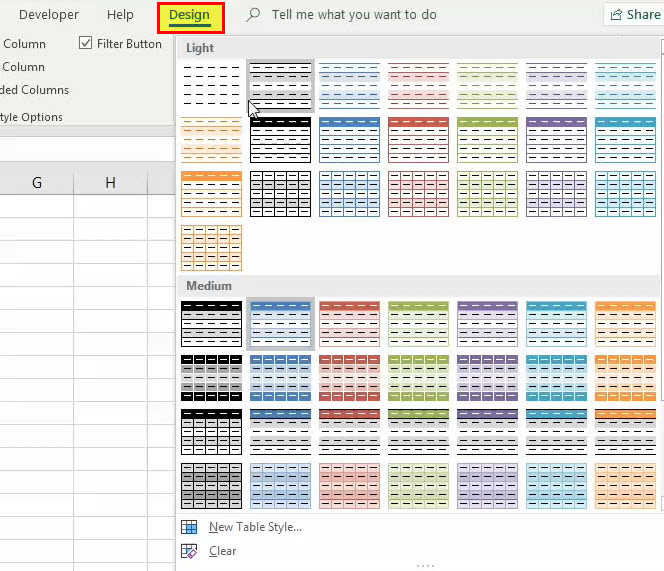
Step 2: Choose the desired color (or style) from the “table styles” group of the Design tab. To expand the list of table styles, click the “more” button displayed at the bottom right side. One can also click “new table style” to view more styles.
The following image shows the expanded list of table styles. Once the desired style is chosen, it will be applied to the entire table.
Note: The default table style of the workbook can be changed by the user. For making this change, perform the listed steps:
- Select the desired table style from the list of table styles.
- Right-click the selected table style and choose “set as default” from the context menu.
What are the Advantages of Creating Tables in Excel?
Let us discuss eight advantages of creating tables in Excel.
#1–Creates Structured References Automatically
An Excel table uses structured referencesIn Excel, structured references define data sets in columns by giving names instead of cell address. You may use the column name instead of the cell address in the formula; this makes work easier.read more for referencing one or more cells. This is in contrast with the direct cell addresses used in a normal data range. A structured reference is a combination of table and column names that are used in Excel formulasThe term «basic excel formula» refers to the general functions used in Microsoft Excel to do simple calculations such as addition, average, and comparison. SUM, COUNT, COUNTA, COUNTBLANK, AVERAGE, MIN Excel, MAX Excel, LEN Excel, TRIM Excel, IF Excel are the top ten excel formulas and functions.read more.
The major benefits of using structured references are listed as follows:
- They automatically update when new entries are added or deleted from the table.
- They are automatically created when one or more cells of the table are selected.
- They can be used both within and outside the table, thus making it easy to locate tables in a workbook.
- They are used to autofill the calculated columns. A calculated column is an additional column added to the existing Excel table. It uses a single formula that expands on its own in the remaining part of the column. This implies that when a formula is entered in one cell of a calculated column, it need not be dragged to the remaining cells of the column. Rather, the formula is automatically entered in all cells (called autofill), unlike a usual data range which requires one to drag the fill handleThe fill handle in Excel allows you to avoid copying and pasting each value into cells and instead use patterns to fill out the information. This tiny cross is a versatile tool in the Excel suite that can be used for data entry, data transformation, and many other applications.read more.
Example of point “d”: The range A2:B7 is an Excel table containing random numbers. To create column C as a calculated column, enter the SUM formula in cell C3, which adds the numbers of cells A3 and B3. Use structured references in this formula. Once the formula is entered, press the “Enter” key. The outcomes are stated as follows:
- The table (A2:B7) automatically expands to include column C.
- The range C4:C7 is automatically filled with the totals of each row of the table.
The preceding results will be obtained with both structured and regular references. This is because autofilling is a feature of Excel tables. However, with structured references, it is easy to read and understand the formula.
Note that if the user makes a change to the formula of the calculated column, the change is automatically replicated in the entire column.
Example of structured references: In the following image, structured references have been used in the SUMIF formula. The “Calls_Table” is the name of the Excel table. “Day” and “duration” are the names of columns A and E respectively. The cell G2 is a direct cell referenceCell reference in excel is referring the other cells to a cell to use its values or properties. For instance, if we have data in cell A2 and want to use that in cell A1, use =A2 in cell A1, and this will copy the A2 value in A1.read more.
Note: In the following image, the black line pointing to cell G2 has been incorrectly placed. It should have pointed to “day,” which is the name of column A. So, please ignore the misplacement.

#2–Is Dynamic in Nature
Any new insertions to the cells below or to the right of the table are automatically included in the Excel table. This implies that the table expands to include such insertions. Likewise, the table contracts when one or more rows and/or columns are deleted from it. Due to automatic expansion and contraction, an Excel table is often considered a dynamic tableDynamic tables in Excel are ones in which the table automatically adjusts its size when a new value is inserted. It can be done in one of two ways: by using the offset function or by creating a data table from the table section.read more.
Expansion implies that the style, formatting, and formulas of the table are automatically applied to the new entries as well. This eliminates the need to format and edit the formulas of individual cells. By default, the formatting stays uniform throughout an Excel table.
Note that the formulas of the table are adjustable as they take into account structured references. In contrast, the formulas of a normal data range do not adjust with insertions or deletions of entries.
Note: To undo table expansion, press the keys “Ctrl+Z” together.
#3–Makes it Easy to Work With PivotTables
It is advised to create a PivotTableA Pivot Table is an Excel tool that allows you to extract data in a preferred format (dashboard/reports) from large data sets contained within a worksheet. It can summarize, sort, group, and reorganize data, as well as execute other complex calculations on it.read more from an Excel table. The major reasons the source data should be an Excel table are listed as follows:
- A PivotTable automatically updates with any changes in the source table. Since Excel tables are dynamic, the data range of the PivotTable also becomes dynamic.
- A single cell of the source table can be selected prior to inserting a PivotTable. In contrast, when the source data is a usual data range, the entire range (or dataset) needs to be selected prior to inserting a PivotTable.
For instance, in the following image, a single cell of the source table has been selected before clicking the “PivotTable” option from the Excel Insert tabIn excel “INSERT” tab plays an important role in analyzing the data. Like all the other tabs in the ribbon INSERT tab offers its own features and tools. Under Insert Tab we have several other groups including tables, illustration, add-ins, charts, Power map, sparklines, filters, etc.read more. Notice that in “table/range,” the name of the source table is reflected.

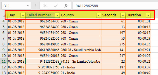
When one scrolls downwards in a worksheet, the table headers are visible at all times. This is because these headers are automatically fixed or frozen at their respective places.
Fixed headers prevent the user from going back to the top row (row 1) again and again. Such frozen headers can be seen within a red rectangle in the following image.
Notice that the user has scrolled downwards such that rows 4 to 13 are visible along with the header row.
Note: To see the frozen header row, ensure that a cell of the table is selected before scrolling.
#5–Helps add a Total Row Containing Functions
An Excel table shows various functions in the total row. For displaying this row, perform the following steps:
- Select any cell of the Excel table. The Design tab appears on the Excel ribbon.
- From the Design tab, select the checkbox of “total row” displayed in the “table style options” group.
The total row is added immediately below the Excel table. Select any cell of this row to see a drop-down arrow on the right side. When this arrow is clicked, a list containing functions appears, as shown in the following image.
Once a function is selected from the list, the respective formula is automatically entered and the output is shown in a cell of the total row.
Notice that row 9 of the following image is the total row. Further, if a function is selected in cell D9, the corresponding output will also be displayed in this cell. The formula will be visible in the formula bar of the worksheet.

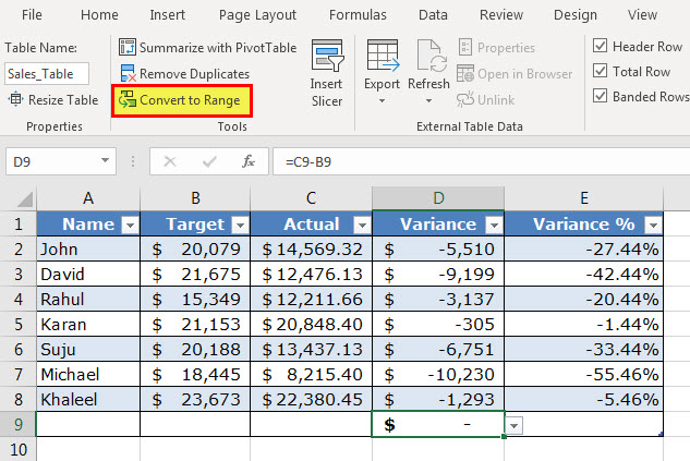
#6–Eases Restoring to Usual Data Range Without Losing the Table Style
An Excel table can be quickly converted to a usual data range. This serves as a benefit when the user requires only the table style and not the functionality of the table. For such conversion, follow either of the listed steps:
- Select any cell of the table. From the Design tab, click “convert to range” in the tools group.
- Select any cell of the table and right-click it. From the context menu, choose “table” followed by “convert to range.”
The “convert to range” feature of the first pointer is shown in the following image. Once an Excel table is converted to a usual data range, the existing structured references are replaced with the regular cell references. However, the data and formatting of the table are retained in the usual data range.
Note: The “convert to range” feature can be used only when the data to be converted is in the form of an Excel table.
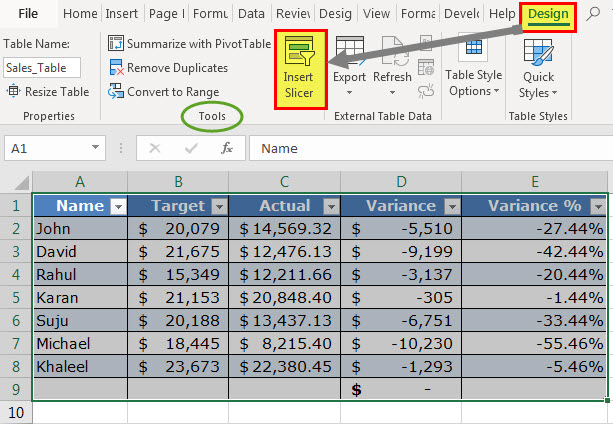
#7–Helps add Slicers for Filtering Data
A slicer helps filter the data of an Excel table. It displays buttons that can be selected or deselected to indicate whether an item is included or excluded from the filter.
Slicers are available in Excel 2013 and the newer Excel versions. The steps to add a slicer to a table are listed as follows:
- Select either a cell within the table or the entire table.
- From the Design tab, select “insert slicer” from the “tools” group.
- The “insert slicer” dialog box opens. Next, select the checkboxes of the columns for which the slicer needs to be created.
- Click “Ok.”
One can have a slicer for each column of the Excel table. Once slicers appear in the worksheet, they can be moved, resized, and formatted according to the requirement.
With a slicer, one can filter and view only particular items (or entries) of the table. To view multiple items of a column, press and hold the “Ctrl” key while selecting the items in the respective slicer.
The following image shows the “insert slicer” option of the Design tab.
Note 1: A slicer can also be added from the “filters” group of the Insert tab of Excel. Click “slicer” in this group and thereafter follow the steps “c” and “d” listed above.
Note 2: A slicer can be used only if the data is in the form of an Excel table.
#8–Assists in Creating Reports in Power BI
Excel tables serve as a source from which data is entered in the Power BI tool. Power BI is a business intelligence tool that helps convert unrelated sources of data into meaningful reports and dashboards. The process of creating reports works as follows:
- Create and upload Excel tables to Power BI.
- Create a report in Power BI by adding visualizations.
- Share the report with other Power BI users or office colleagues.
Excel tables are a preferred data source in Power BI due to the following reasons:
- They allow quick access to the tabular format of the dataset.
- They help ease comparisons within a dataset.
- They can be easily edited and organized prior to being uploaded in Power BI.
How to Turn off Structured References in Excel?
The steps to turn off structured references in Excel are listed as follows:
Step 1: Click the File tab of Excel. It is displayed within a red box in the following image.

Step 2: Select “options” shown in the following image.
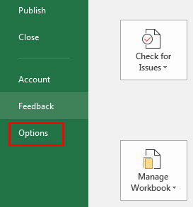
Step 3: The “Excel options” dialog box opens. Click “formulas” appearing on the left side of the window. Deselect the checkbox of “use table names in formulas.” This is shown in the following image.
Next, click “Ok.” The structured references will be turned off in Excel.
Note: By changing this setting, the structured references used in the existing formulas of the Excel table are not removed. However, the new formulas applied to the table will contain regular cell references instead of structured references. If regular cell references are required in existing formulas too, they will have to be edited manually.
Further, whether the structured references are turned on or off, the changed setting will be applied to all workbooks that the user is working on.

Frequently Asked Questions
1. What are Excel tables and how are they created?
An Excel table displays the data in a tabulated format. Every column should have unique headers (or names) according to the kind of data they contain. Such headers are placed in the top row of the table. The table may or may not be named by the user.
If the columns and table are not named by the user, Excel assigns default names to both of them. These names are used as structured references in all formulas applied within or outside the table (that contain a table reference).
To create a table in Excel, select any cell of the dataset and press the keys “Ctrl+T” or “Ctrl+L.”
2. How to join two tables in Excel?
Two tables that have a common column can be joined with the help of the VLOOKUP function of Excel. The formula is stated as follows:
“=VLOOKUP(lookup_value,entire_lookup_table,return_column,FALSE)”
For instance, the first table is named “table1” and the second table is named “table2.” To pull the data of a single column of “table2” in “table1,” enter the following formula:
“=VLOOKUP($A2,table2,3,FALSE)”
This formula looks up the value of cell A2 in “table2.” It returns an exact match from the third column of “table2.”
One can use either regular or structured references in the given formula. By selecting the cell of the “lookup_value” and the range of the “entire_lookup_table,” Excel will automatically enter structured references in the VLOOKUP formula.
Note 1: Enter the given formula in the first cell to the immediate right of the first table. Once entered, press the “Enter” key. The Excel table expands to include the new column. Consequently, the outputs of the entire column are displayed in the first table.
Note 2: For the given formula to work, the column containing the “lookup_value” should be common to both tables. Moreover, the lookup column (containing the “lookup_value”) should be the leftmost column of the second table. The return column (containing the value to be returned) of the second table should be to the right of the lookup column.
3. When should Excel tables be used and how to locate them in a workbook?
Excel tables should be used in the following situations:
• To arrange data in a tabular format
• To facilitate comparisons of data values
• To improve the readability of the dataset
• To ease data analysis and eventually assist in decision-making
To locate tables in a workbook, click the downward arrow appearing on the right side of the name box. It shows the names of all the tables of the workbook. Clicking on any of these names will select that particular table.
Recommended Articles
This has been a guide to tables in Excel. Here, we explain how to create/insert/customize Excel tables along with examples and advantages. You may also look at these useful functions of Excel–
- Delete Pivot Table ExcelTo delete a pivot table in Excel, you must first select it. Then go to the Analyze menu tab under the Design and Analyze menu tabs and select actions. Then, from the Select option’s drop-down option, select Entire Pivot Table to delete it.read more
- Refresh Pivot Table in ExcelTo refresh pivot tables, you may use the following methods — refresh pivot table by changing data source, refresh pivot table using right click option, auto-refresh pivot table using VBA Code, refresh pivot table when you open the workbook.read more
- Data Table in Excel
- Excel Merge Tables We can use a number of different methods to merge tables in Excel, including the VLOOKUP function, the INDEX function, and the MATCH function.read more