
Динамический диапазон с автоподстройкой размеров
Есть ли у вас таблицы с данными в Excel, размеры которых могут изменяться, т.е. количество строк (столбцов) может увеличиваться или уменьшаться в процессе работы? Если размеры таблицы «плавают», то придется постоянно мониторить этот момент и подправлять:
- ссылки в формулах отчетов, которые ссылаются на нашу таблицу
- исходные диапазоны сводных таблиц, которые построены по нашей таблице
- исходные диапазоны диаграмм, построенных по нашей таблице
- диапазоны для выпадающих списков, которые используют нашу таблицу в качестве источника данных
Все это в сумме не даст вам скучать 
Гораздо удобнее и правильнее будет создать динамический «резиновый» диапазон, который автоматически будет подстраиваться в размерах под реальное количество строк-столбцов данных. Чтобы реализовать такое, есть несколько способов.
Способ 1. Умная таблица
Выделите ваш диапазон ячеек и выберите на вкладке Главная – Форматировать как Таблицу (Home – Format as Table):

Если вам не нужен полосатый дизайн, который добавляется к таблице побочным эффектом, то его можно отключить на появившейся вкладке Конструктор (Design). Каждая созданная таким образом таблица получает имя, которое можно заменить на более удобное там же на вкладке Конструктор (Design) в поле Имя таблицы (Table Name).

Теперь можно использовать динамические ссылки на нашу «умную таблицу»:
- Таблица1 – ссылка на всю таблицу кроме строки заголовка (A2:D5)
- Таблица1[#Все] – ссылка на всю таблицу целиком (A1:D5)
- Таблица1[Питер] – ссылка на диапазон-столбец без первой ячейки-заголовка (C2:C5)
- Таблица1[#Заголовки] – ссылка на «шапку» с названиями столбцов (A1:D1)
Такие ссылки замечательно работают в формулах, например:
=СУММ(Таблица1[Москва]) – вычисление суммы по столбцу «Москва»
или
=ВПР(F5;Таблица1;3;0) – поиск в таблице месяца из ячейки F5 и выдача питерской суммы по нему (что такое ВПР?)
Такие ссылки можно успешно использовать при создании сводных таблиц, выбрав на вкладке Вставка – Сводная таблица (Insert – Pivot Table) и введя имя умной таблицы в качестве источника данных:

Если выделить фрагмент такой таблицы (например, первых два столбца) и создать диаграмму любого типа, то при дописывании новых строк они автоматически будут добавляться к диаграмме.
При создании выпадающих списков прямые ссылки на элементы умной таблицы использовать нельзя, но можно легко обойти это ограничение с помощью тактической хитрости – использовать функцию ДВССЫЛ (INDIRECT), которая превращает текст в ссылку:

Т.е. ссылка на умную таблицу в виде текстовой строки (в кавычках!) превращается в полноценную ссылку, а уж ее выпадающий список нормально воспринимает.
Способ 2. Динамический именованный диапазон
Если превращение ваших данных в умную таблицу по каким-либо причинам нежелательно, то можно воспользоваться чуть более сложным, но гораздо более незаметным и универсальным методом – создать в Excel динамический именованный диапазон, ссылающийся на нашу таблицу. Потом, как и в случае с умной таблицей, можно будет свободно использовать имя созданного диапазона в любых формулах, отчетах, диаграммах и т.д. Для начала рассмотрим простой пример:

Задача: сделать динамический именованный диапазон, который ссылался бы на список городов и автоматически растягивался-сжимался в размерах при дописывании новых городов либо их удалении.
Нам потребуются две встроенных функции Excel, имеющиеся в любой версии – ПОИКСПОЗ (MATCH) для определения последней ячейки диапазона и ИНДЕКС (INDEX) для создания динамической ссылки.
Ищем последнюю ячейку с помощью ПОИСКПОЗ
ПОИСКПОЗ(искомое_значение;диапазон;тип_сопоставления) – функция, которая ищет заданное значение в диапазоне (строке или столбце) и выдает порядковый номер ячейки, где оно было найдено. Например, формула ПОИСКПОЗ(“март”;A1:A5;0) выдаст в качестве результата число 4, т.к. слово «март» расположено в четвертой по счету ячейке в столбце A1:A5. Последний аргумент функции Тип_сопоставления = 0 означает, что мы ведем поиск точного соответствия. Если этот аргумент не указать, то функция переключится в режим поиска ближайшего наименьшего значения – это как раз и можно успешно использовать для нахождения последней занятой ячейки в нашем массиве.
Суть трюка проста. ПОИСКПОЗ перебирает в поиске ячейки в диапазоне сверху-вниз и, по идее, должна остановиться, когда найдет ближайшее наименьшее значение к заданному. Если указать в качестве искомого значение заведомо больше, чем любое имеющееся в таблице, то ПОИСКПОЗ дойдет до самого конца таблицы, ничего не найдет и выдаст порядковый номер последней заполненной ячейки. А нам это и нужно!
Если в нашем массиве только числа, то можно в качестве искомого значения указать число, которое заведомо больше любого из имеющихся в таблице:

Для гарантии можно использовать число 9E+307 (9 умножить на 10 в 307 степени, т.е. 9 с 307 нулями) – максимальное число, с которым в принципе может работать Excel.
Если же в нашем столбце текстовые значения, то в качестве эквивалента максимально большого числа можно вставить конструкцию ПОВТОР(“я”;255) – текстовую строку, состоящую из 255 букв «я» — последней буквы алфавита. Поскольку при поиске Excel, фактически, сравнивает коды символов, то любой текст в нашей таблице будет технически «меньше» такой длинной «яяяяя….я» строки:

Формируем ссылку с помощью ИНДЕКС
Теперь, когда мы знаем позицию последнего непустого элемента в таблице, осталось сформировать ссылку на весь наш диапазон. Для этого используем функцию:
ИНДЕКС(диапазон; номер_строки; номер_столбца)
Она выдает содержимое ячейки из диапазона по номеру строки и столбца, т.е. например функция =ИНДЕКС(A1:D5;3;4) по нашей таблице с городами и месяцами из предыдущего способа выдаст 1240 – содержимое из 3-й строки и 4-го столбца, т.е. ячейки D3. Если столбец всего один, то его номер можно не указывать, т.е. формула ИНДЕКС(A2:A6;3) выдаст «Самару» на последнем скриншоте.
Причем есть один не совсем очевидный нюанс: если ИНДЕКС не просто введена в ячейку после знака =, как обычно, а используется как финальная часть ссылки на диапазон после двоеточия, то выдает она уже не содержимое ячейки, а ее адрес! Таким образом формула вида $A$2:ИНДЕКС($A$2:$A$100;3) даст на выходе уже ссылку на диапазон A2:A4.
И вот тут в дело вступает функция ПОИСКПОЗ, которую мы вставляем внутрь ИНДЕКС, чтобы динамически определить конец списка:
=$A$2:ИНДЕКС($A$2:$A$100; ПОИСКПОЗ(ПОВТОР(«я»;255);A2:A100))
Создаем именованный диапазон
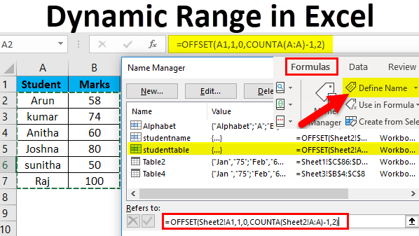
Осталось упаковать все это в единое целое. Откройте вкладку Формулы (Formulas) и нажмите кнопку Диспетчер Имен (Name Manager). В открывшемся окне нажмите кнопку Создать (New), введите имя нашего диапазона и формулу в поле Диапазон (Reference):

Осталось нажать на ОК и готовый диапазон можно использовать в любых формулах, выпадающих списках или диаграммах.
Ссылки по теме
- Использование функции ВПР (VLOOKUP) для связывания таблиц и подстановки значений
- Как создать автоматически наполняющийся выпадающий список
- Как создать сводную таблицу для анализа большого массива данных
Excel Dynamic Range (Table of Contents)
- Dynamic Range in Excel
- Uses of Dynamic Range
- How to Create a Dynamic Range in Excel?
Dynamic Range in Excel
Dynamic Range in excel allows us to use the newly updated range always whenever the new set of lines are appended in the data. It just gets updated automatically when we add new cells or rows. We have used a static range where value cells are fixed, and herewith a Dynamic range, our range will change as well add the data. This can be done in any function in excel. And for this, we have an option in excel available in the Formula tab under defined names as Name Manager.
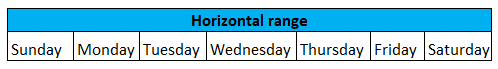
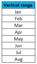
Below are the examples for range:
Uses of Dynamic Range
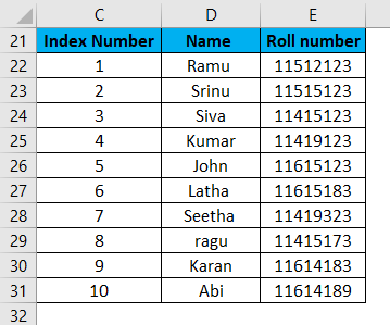
Let’s assume you have to give an index number for a database range of 100 rows. As we have 100 rows, we need to give 100 index numbers vertically from top to bottom. Suppose we type that 100 numbers manually; it will take around 5-10 minutes of time. Here range helps to make this task within 5 seconds of time. Let’s see how it will work.
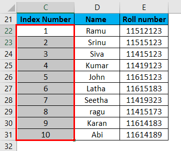
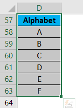
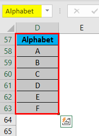
We need to achieve the index numbers as shown in the below screenshot; here, I give an example only for 10 rows.
Give the first two numbers under the index number, select the range of two numbers as shown below, and click on the corner (Marked in red colour).
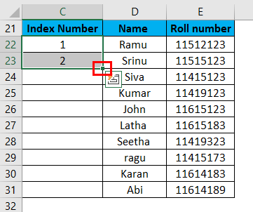
Drag until the required range. It will give the continuous series as per the first two numbers pattern.
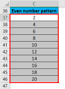
If we give the first cell as 2 and the second cell as 4, then it will give all the even numbers. Select the range of two numbers as shown below and click on the corner (Marked in red colour).
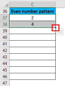
Drag until the required range. It will give the continuous series as per the first two numbers pattern.
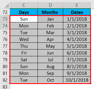
The same will apply for months, days, dates etc.…Provide the first two values of the required pattern, highlight the range, and then click on the corner.
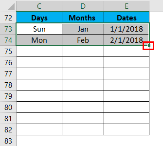
Drag until the required length. It will give the continuous series as per the first two numbers pattern.
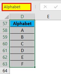
I hope you understand what it is a range; now, we will discuss the dynamic range. You can give a name to a range of cells by simply selecting the range.
Give the name in the name box (highlighted in the screenshot).
Please select the Name which we added and press enter.
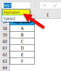
So that when you select that name, the range will pick automatically.
Dynamic Range in Excel
Dynamic range is nothing but the range that picked dynamically when additional data is added to the existing range.
Example
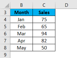
See the below sales chart of a company from Jan to Apr.
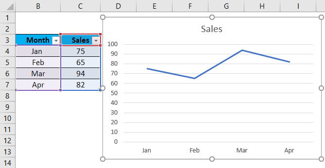
When we update May below the Apr month data’s sales in May month, the sales chart will update automatically (Dynamically). This is happening because the range we used is dynamic range; hence, the chart takes the dynamic range and changes the chart accordingly.

If the range is not a dynamical range, then the chart will not automatically update when we update the data to the existing data range.
We can achieve the Dynamic range in two ways.
- Using Excel table feature
- Using Offsetting entry
How to Create a Dynamic Range in Excel?
Dynamic range in Excel is straightforward and easy to correct. Let’s understand how to Create a Dynamic range with some Examples.
You can download this Dynamic Range Excel Template here – Dynamic Range Excel Template
Dynamic Range in Excel Example #1 – Excel Table feature
We can achieve the Dynamic range by using this feature, but this will apply if we use the excel version of 2017 and the versions released after 2017.
Let’s see how to create now. Take a database range like below.
Select the entire data range and click on the insert button at the top menu bar marked in red colour.
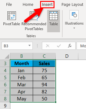
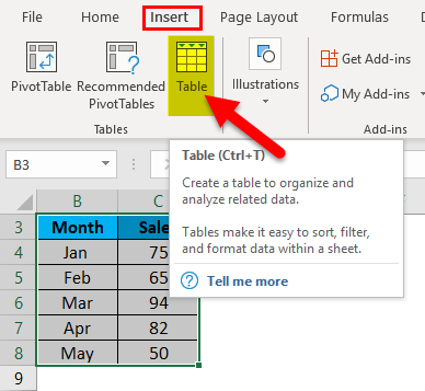
Later click on the table below the insert menu.
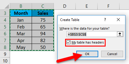
The below-shown pop up will come; check the field ‘My table has header’ as our selected data table range has a header and Click ‘Ok’.
Then the data format will change to table format; you can observe the colour also.

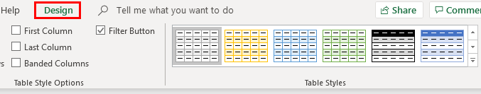
If you want to change the format(colour), select the table and click on the top menu bar’s design button. You can select the required formats from the ‘table styles’.
Now the data range is in table format; hence whenever you add new data lines, the table feature makes the data range update dynamically into a table; hence the chart also changes dynamically. Below is the screenshot for reference.
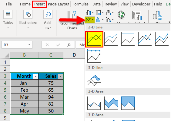
Click on insert and go to charts and Click on Line chart as shown below.
A-Line Chart is added, as shown below.
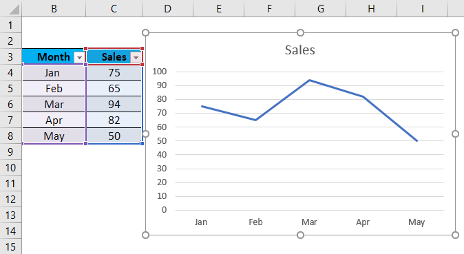
If you add one more data to the table, i.e. Jun and sales as 100, then the chart is automatically updated.

This is one way of creating a dynamical data range.
Dynamic Range in Excel Example #2 – Using the offsetting entry
The offsetting formula helps to start with a reference point and can offset down with the required number of rows and right or left with required numbers of columns into our table range.
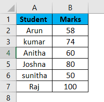
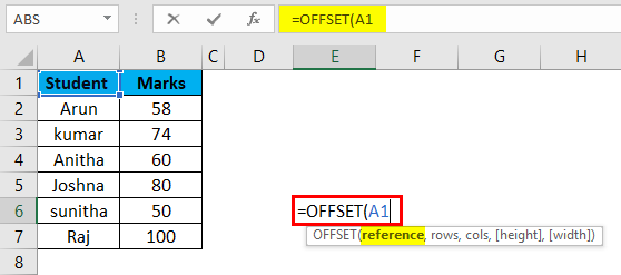
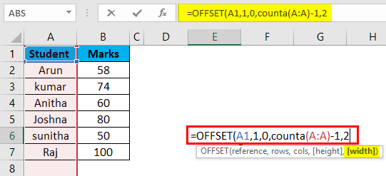
Let’s see how to achieve dynamic range using the offsetting formula. Below is the data sample of the student table for creating a dynamic range.
To explain to you the format of offset, I am giving the formula in the normal sheet instead of applying it in the “Define name”.
Offset entry format
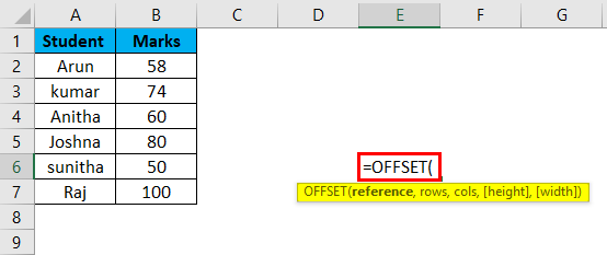
- Reference: Refers to the reference cell of the table range, which is the starting point.
- Rows: Refers to the required number of rows to offset below the starting reference point.
- Cols: Refers to the required number of columns to offset right or left to the starting point.
- Height: Refers to the height of the rows.
- Width: Refers to the Width of the columns.
Start with the reference cell, where a student is the reference cell where you want to start a data range.
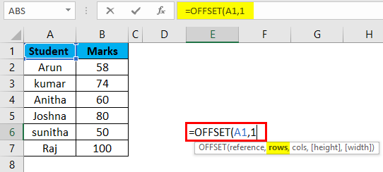
Now give the required number of rows to go down to consider into the range. Here ‘1’ is given because it is one row down from the reference cell.
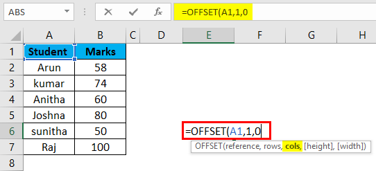
Now give the columns as 0 as we are not going to consider the columns here.
Now give the height of rows as we are not sure how many rows we will add in the future; hence, give the ‘counta’ function of rows (select the entire ‘A’ column). But we are not treating the header into range, so reduce by 1.
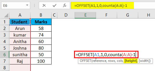
Now in Width, give 2 as here we have two columns, and we do not want to add any additional columns here. In case if we are not aware of how many columns we are going to add in future, then apply the ‘counta’ function to the entire row as how we applied to height. Close the formula.
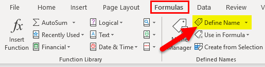
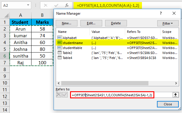
Now we need to apply the offset formula in the defined name to create a dynamic range. Click on the “formula” menu at the top (highlighted).
Click on the option “Define Name “ marked in the below screenshot.
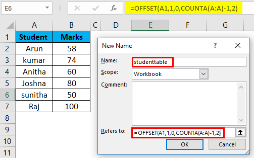
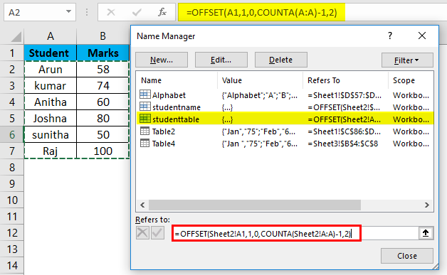
A popup will come, give the name of table range as ‘student table without space. ‘Scope’ leave it like a ‘Workbook’ and then go to ‘Refers to’ where we need to give the “OFFSET” formula. Copy the formula which we prepared priory and paste in Refers to
Now we can check the range by clicking on the Name manager and select the Name you provided in the Define name.
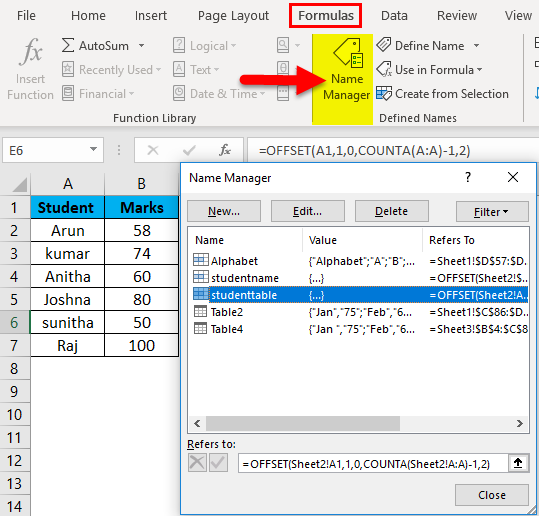
Here it is “Studenttable”, and then click on the formula to automatically highlight the table range, as you can observe in the screenshot.
If we add another line item to the existing range, the range will pick automatically. You can check by adding a line item and check the range; below is the example screenshot.
I hope you understand how to work with the Dynamic range.
Advantages of Dynamic Range in Excel
- Instant updating of Charts, Pivots etc…
- No need for manual updating of formulas.
Disadvantages of Dynamic Range in Excel
- When working with a centralized database with multiple users, update the correct data as the range picks automatically.
Things to Remember About Dynamic Range in Excel
- Dynamic range is used when needing updating of data dynamically.
- Excel table feature and OFFSET formula help to achieve dynamic range.
Recommended Articles
This has been a guide to Dynamic Range in Excel. Here we discuss the Meaning of Range and how to Create a Dynamic Range in Excel with examples and downloadable excel templates. You may also look at these useful functions in excel –
- How to Use the INDIRECT Function in Excel?
- Guide to HLOOKUP Function in Excel
- Guide to Excel TREND Function
- Excel Forecast Function -MS Excel
In this Article
- Referencing Ranges and Cells
- Range Property
- Cells Property
- Dynamic Ranges with Variables
- Last Row in Column
- Last Column in Row
- SpecialCells – LastCell
- UsedRange
- CurrentRegion
- Named Range
- Tables
This article will demonstrate how to create a Dynamic Range in Excel VBA.
Declaring a specific range of cells as a variable in Excel VBA limits us to working only with those particular cells. By declaring Dynamic Ranges in Excel, we gain far more flexibility over our code and the functionality that it can perform.
Referencing Ranges and Cells
When we reference the Range or Cell object in Excel, we normally refer to them by hardcoding in the row and columns that we require.
Range Property
Using the Range Property, in the example lines of code below, we can perform actions on this range such as changing the color of the cells, or making the cells bold.
Range("A1:A5").Font.Color = vbRed
Range("A1:A5").Font.Bold = True
Cells Property
Similarly, we can use the Cells Property to refer to a range of cells by directly referencing the row and column in the cells property. The row has to always be a number but the column can be a number or can a letter enclosed in quotation marks.
For example, the cell address A1 can be referenced as:
Cells(1,1)Or
Cells(1, "A")To use the Cells Property to reference a range of cells, we need to indicate the start of the range and the end of the range.
For example to reference range A1: A6 we could use this syntax below:
Range(Cells(1,1), Cells(1,6)We can then use the Cells property to perform actions on the range as per the example lines of code below:
Range(Cells(2, 2), Cells(6, 2)).Font.Color = vbRed
Range(Cells(2, 2), Cells(6, 2)).Font.Bold = True
Dynamic Ranges with Variables
As the size of our data changes in Excel (i.e. we use more rows and columns that the ranges that we have coded), it would be useful if the ranges that we refer to in our code were also to change. Using the Range object above we can create variables to store the maximum row and column numbers of the area of the Excel worksheet that we are using, and use these variables to dynamically adjust the Range object while the code is running.
For example
Dim lRow as integer
Dim lCol as integer
lRow  = Range("A1048576").End(xlUp).Row
lCol  = Range("XFD1").End(xlToLeft).Column
Last Row in Column
As there are 1048576 rows in a worksheet, the variable lRow will go to the bottom of the sheet and then use the special combination of the End key plus the Up Arrow key to go to the last row used in the worksheet – this will give us the number of the row that we need in our range.
Last Column in Row
Similarly, the lCol will move to Column XFD which is the last column in a worksheet, and then use the special key combination of the End key plus the Left Arrow key to go to the last column used in the worksheet – this will give us the number of the column that we need in our range.
Therefore, to get the entire range that is used in the worksheet, we can run the following code:
Sub GetRange()
  Dim lRow As Integer
  Dim lCol As Integer
  Dim rng As Range
  lRow = Range("A1048576").End(xlUp).Row
'use the lRow to help find the last column in the range
  lCol = Range("XFD" & lRow).End(xlToLeft).Column
  Set rng = Range(Cells(1, 1), Cells(lRow, lCol))
'msgbox to show us the range
  MsgBox "Range is " & rng.Address
End Sub
VBA Coding Made Easy
Stop searching for VBA code online. Learn more about AutoMacro — A VBA Code Builder that allows beginners to code procedures from scratch with minimal coding knowledge and with many time-saving features for all users!

Learn More
SpecialCells – LastCell
We can also use SpecialCells method of the Range Object to get the last row and column used in a Worksheet.
Sub UseSpecialCells()
  Dim lRow As Integer
  Dim lCol As Integer
  Dim rng As Range
  Dim rngBegin As Range
  Set rngBegin = Range("A1")
  lRow = rngBegin.SpecialCells(xlCellTypeLastCell).Row
  lCol = rngBegin.SpecialCells(xlCellTypeLastCell).Column
  Set rng = Range(Cells(1, 1), Cells(lRow, lCol))
'msgbox to show us the range
  MsgBox "Range is " & rng.Address
End Sub
UsedRange
The Used Range Method includes all the cells that have values in them in the current worksheet.
Sub UsedRangeExample()
  Dim rng As Range
  Set rng = ActiveSheet.UsedRange
'msgbox to show us the range
  MsgBox "Range is " & rng.Address
End Sub
CurrentRegion
The current region differs from the UsedRange in that it looks at the cells surrounding a cell that we have declared as a starting range (ie the variable rngBegin in the example below), and then looks at all the cells that are ‘attached’ or associated to that declared cell. Should a blank cell in a row or column occur, then the CurrentRegion will stop looking for any further cells.
Sub CurrentRegion()
  Dim rng As Range
  Dim rngBegin As Range
  Set rngBegin = Range("A1")
  Set rng = rngBegin.CurrentRegion
'msgbox to show us the range
  MsgBox "Range is " & rng.Address
End Sub
If we use this method, we need to make sure that all the cells in the range that you require are connected with no blank rows or columns amongst them.
VBA Programming | Code Generator does work for you!
Named Range
We can also reference Named Ranges in our code. Named Ranges can be dynamic in so far as when data is updated or inserted, the Range Name can change to include the new data.
This example will change the font to bold for the range name “January”
Sub RangeNameExample()
  Dim rng as Range
  Set rng = Range("January")
  rng.Font.Bold = = True
End Sub
As you will see in the picture below, if a row is added into the range name, then the range name automatically updates to include that row.
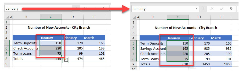
Should we then run the example code again, the range affected by the code would be C5:C9 whereas in the first instance it would have been C5:C8.
Tables
We can reference tables (click for more information about creating and manipulating tables in VBA) in our code. As a table data in Excel is updated or changed, the code that refers to the table will then refer to the updated table data. This is particularly useful when referring to Pivot tables that are connected to an external data source.
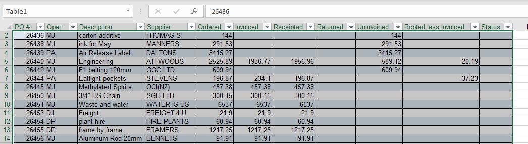
Using this table in our code, we can refer to the columns of the table by the headings in each column, and perform actions on the column according to their name. As the rows in the table increase or decrease according to the data, the table range will adjust accordingly and our code will still work for the entire column in the table.
For example:
Sub DeleteTableColumn()
  ActiveWorkbook.Worksheets("Sheet1").ListObjects("Table1").ListColumns("Supplier").Delete
End Sub
Если вам необходимо постоянно добавлять значения в столбец, то для правильной работы Ваших формул, Вам наверняка понадобятся динамические диапазоны, которые автоматически увеличиваются или уменьшаются в зависимости от количества ваших данных.
Динамический диапазон —
это
Именованный диапазон
с изменяющимися границами. Границы диапазона изменяются в зависимости от количества значений в определенном диапазоне.
Динамические диапазоны используются для создания таких структур, как:
Выпадающий (раскрывающийся) список
,
Вложенный связанный список
и
Связанный список
.
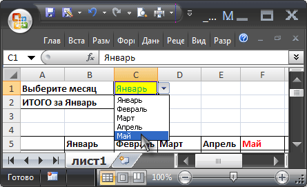
Задача
Имеется таблица продаж по месяцам некоторых товаров (см.
Файл примера
):
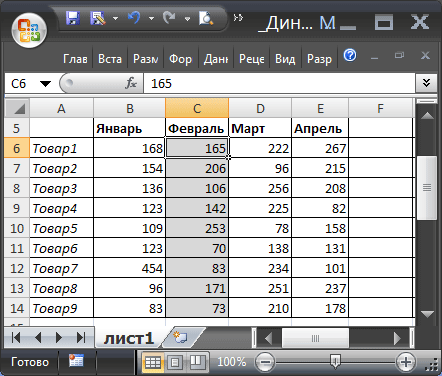
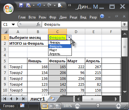
Необходимо найти сумму продаж товаров в определенном месяце. Пользователь должен иметь возможность выбрать нужный ему месяц и получить итоговую сумму продаж. Выбор месяца пользователь должен осуществлять с помощью
Выпадающего списка
.
Для решения задачи нам потребуется сформировать два
динамических диапазона
: один для
Выпадающего списка
, содержащего месяцы; другой для диапазона суммирования.
Для формирования динамических диапазонов будем использовать функцию
СМЕЩ()
, которая возвращает ссылку на диапазон в зависимости от значения заданных аргументов. Можно задавать высоту и ширину диапазона, а также смещение по строкам и столбцам.
Создадим
динамический диапазон
для
Выпадающего списка
, содержащего месяцы. С одной стороны нужно учитывать тот факт, что пользователь может добавлять продажи за следующие после апреля месяцы (май, июнь…), с другой стороны
Выпадающий список
не должен содержать пустые строки.
Динамический диапазон
как раз и служит для решения такой задачи.
Для создания динамического диапазона:
-
на вкладке
Формулы
в группе
Определенные имена
выберите команду
Присвоить имя
; -
в поле
Имя
введите:
Месяц
; -
в поле
Область
выберите лист
Книга
; -
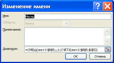
в поле
Диапазон
введите формулу
=СМЕЩ(лист1!$B$5;;;1;СЧЁТЗ(лист1!$B$5:$I$5))
- нажмите ОК.
Теперь подробнее. Любой диапазон в EXCEL задается координатами верхней левой и нижней правой ячейки диапазона. Исходной ячейкой, от которой отсчитывается положение нашего динамического диапазона, является ячейка
B5
. Если не заданы аргументы функции
СМЕЩ()
смещ_по_строкам,
смещ_по_столбцам
(как в нашем случае), то эта ячейка является левой верхней ячейкой диапазона. Нижняя правая ячейка диапазона определяется аргументами
высота
и
ширина
. В нашем случае значение высоты =1, а значение ширины диапазона равно результату вычисления формулы
СЧЁТЗ(лист1!$B$5:$I$5)
, т.е. 4 (в строке 5 присутствуют 4 месяца с
января
по
апрель
). Итак, адрес нижней правой ячейки нашего
динамического диапазона
определен – это
E
5
.
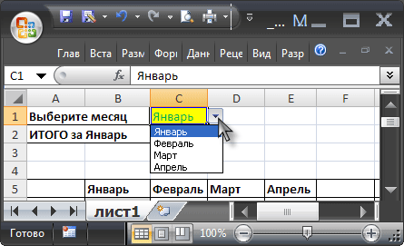
При заполнении таблицы данными о продажах за
май
,
июнь
и т.д., формула
СЧЁТЗ(лист1!$B$5:$I$5)
будет возвращать число заполненных ячеек (количество названий месяцев) и соответственно определять новую ширину динамического диапазона, который в свою очередь будет формировать
Выпадающий список
.
ВНИМАНИЕ! При использовании функции
СЧЕТЗ()
необходимо убедиться в отсутствии пустых ячеек! Т.е. нужно заполнять перечень месяцев без пропусков.
Теперь создадим еще один
динамический диапазон
для суммирования продаж.
Для создания
динамического диапазона
:
-
на вкладке
Формулы
в группе
Определенные имена
выберите команду
Присвоить имя
; -
в поле
Имя
введите:
Продажи_за_месяц
; -
в поле
Диапазон
введите формулу =
СМЕЩ(лист1!$A$6;;ПОИСКПОЗ(лист1!$C$1;лист1!$B$5:$I$5;0);12)
- нажмите ОК.
Теперь подробнее.
Функция
ПОИСКПОЗ()
ищет в строке 5 (перечень месяцев) выбранный пользователем месяц (ячейка
С1
с выпадающим списком) и возвращает соответствующий номер позиции в диапазоне поиска (названия месяцев должны быть уникальны, т.е. этот пример не годится для нескольких лет). На это число столбцов смещается левый верхний угол нашего динамического диапазона (от ячейки
А6
), высота диапазона не меняется и всегда равна 12 (при желании ее также можно сделать также динамической – зависящей от количества товаров в диапазоне).
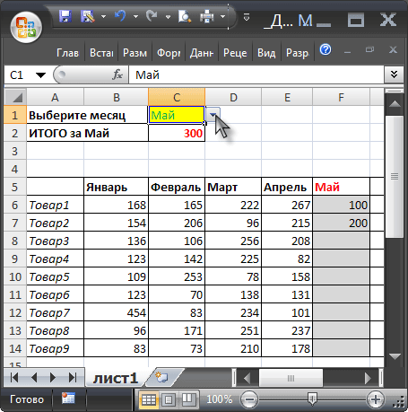
И наконец, записав в ячейке
С2
формулу =
СУММ(Продажи_за_месяц)
получим сумму продаж в выбранном месяце.
Например, в мае.
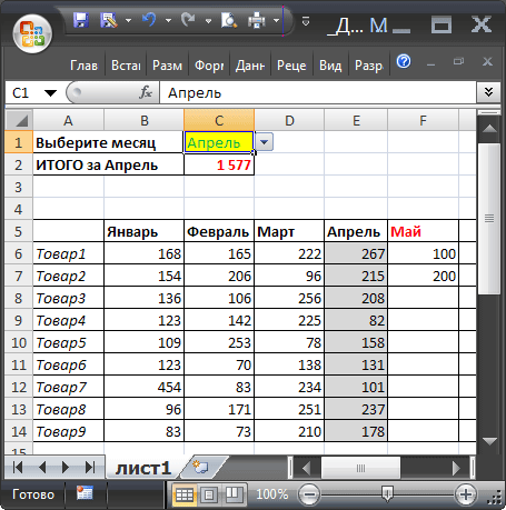
Или, например, в апреле.
Примечание:
Вместо формулы с функцией
СМЕЩ()
для подсчета заполненных месяцев можно использовать формулу с функцией
ИНДЕКС()
: =
$B$5:ИНДЕКС(B5:I5;СЧЁТЗ($B$5:$I$5))
Формула подсчитывает количество элементов в строке 5 (функция
СЧЁТЗ()
) и определяет ссылку на последний элемент в строке (функция
ИНДЕКС()
), тем самым возвращает ссылку на диапазон
B5:E5
.
Визуальное отображение динамического диапазона
Выделить текущий
динамический диапазон
можно с помощью
Условного форматирования
. В
файле примера
для ячеек диапазона
B6:I14
применено правило
Условного форматирования
с формулой: =
СТОЛБЕЦ(B6)=СТОЛБЕЦ(Продажи_за_месяц)
Условное форматирование
автоматически выделяет серым цветом продажи
текущего месяца
, выбранного с помощью
Выпадающего списка
.
Применение динамического диапазона
Примеры использования
динамического диапазона
, например, можно посмотреть в статьях
Динамические диаграммы. Часть5: график с Прокруткой и Масштабированием
и
Динамические диаграммы. Часть4: Выборка данных из определенного диапазона
.
In Excel, a dynamic range is a reference (or a formula you use to create a reference) that may change based on user input or the results of another cell or function. It is more than just a fixed group of cells like $A1:$A100. I use dynamic ranges mostly for customizable drop-down lists. To avoid showing a bunch of blanks in the list, I use a formula to reference a range that extends to the last value in a column. The image below shows 4 different formulas that reference the range A2:A9 and can expand to include more rows if the user adds more categories to the list.
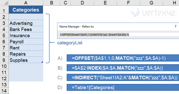
When we talk about a dynamic named range, we’re talking about using the Name Manager (via the Formula tab) to define a name for the formula, such as categoryList. We can then use that Name in other formulas or as the Source for drop-down lists.
This article isn’t about the awesome advantages of using Excel Names, though there are many. Instead, it is about the many different formulas you can use to create the dynamic named ranges.
To see these examples in action, download the Excel file below.
Download the Example File (DynamicRanges.xlsx)
Do you have a Dynamic Named Range challenge you need to solve? If you can’t figure it out after reading this article, go ahead and ask your question by commenting below.
This Page (contents):
- A) The OFFSET Function
- B) The INDEX Function for a Non-Volatile Dynamic Range
- C) The INDIRECT Function
- D) Structured References with Excel Tables
- E) The CHOOSE and IF Functions
- Find the Position of the LAST Value in the Column
- Bonus: Create a Dynamic Print Area
- No Dynamic Named Ranges in Google Sheets
Watch the Video
A) The OFFSET Function
The most common function used to create a dynamic named range is probably the OFFSET function. It allows you to define a range with a specific number of rows and columns, starting from a reference cell. The syntax for the OFFSET function is:
=OFFSET(reference,offset_rows,offset_cols,[height],[width])
The offset_rows and offset_cols values tell the function where you want the upper-left cell of your range to be, relative to the reference cell. The height and width values tell the function how many rows and columns you want to include in your range.
A Basic Customizable List
In the meal planner template, I have a list of meals that I use as the Source for many different drop-down lists. I want to allow the user to edit and add to the list, so the dynamic named range used by the drop-down needs to extend to the last value in the list. I could define the range as $A:$A (the entire column) or $A1:$A1000 (assuming they won’t add more than 1000 items to the list), but then I’d end up with a bunch of blank cells at the end of my drop-down list.
Using the OFFSET function, I define a range that starts at cell $A$1 and ends at the cell containing the last value in the column. If the last value in the column was on row 15, the formula for the named range would be:
=OFFSET($A$1,0,0,15,1)
To make this formula dynamic, I’ll use a formula or reference in place of the height value (15) to specify how many rows I want the range to include. I expect only text values in this list, so I’ll use the MATCH function to find the last text value in the column like this:
=OFFSET($A$1,0,0,MATCH("zzzz",$A:$A),1)
There are many formulas you can use to determine the height or width of the range, such as COUNTA, COUNT, VLOOKUP, LOOKUP, MATCH or various array formulas. What formula you use may depend on whether you expect there to be blank cells in the list, error values (like #N/A or #DIV/0!), or data of different types (text or numeric or both), and whether calculation speed is an issue.
Later in this article I’ll talk more about the various formulas for finding the last value in the range. For now, we’ll continue using MATCH.
A Robust Dynamic Range
When you allow a user to edit a list, they may end up deleting the first row in the list, or they might insert a row above the first row in the list (between the label row and the first item). To create a formula that works in spite of these actions by the user, I like to use a label for the reference and include the label in the range, as shown in the following examples.
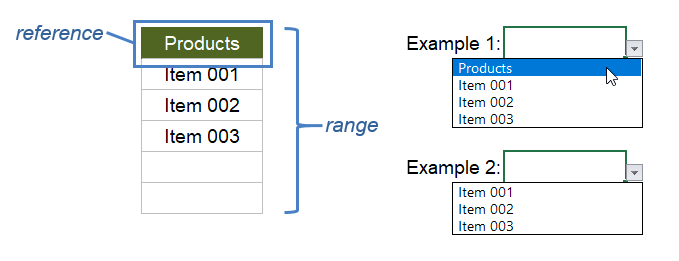
Example 1: Include the label in the list
=OFFSET(reference,0,0,MATCH("zzz",range),1)
Example 2: Exclude the label from the list
=OFFSET(reference,1,0,MATCH("zzz",range)-1,1)
Notice in the second example that reference and range have not changed. To exclude the label from the list, we are using an offset of 1 row and subtracting one row from the number returned by the MATCH function.
B) The INDEX Function for a Non-Volatile Dynamic Range
A volatile function within a cell or named range is recalculated every time any cell in the worksheet recalculates (instead of just when one of the function’s arguments changes). Also, any formula that depends on a cell containing a volatile function is also recalculated. If you have a large file with thousands of inefficient formulas that reference a cell containing a volatile function, Excel may seem to take forever to recalculate. OFFSET is a volatile function. INDEX is not, so some people prefer to use INDEX for dynamic ranges.
The INDEX function can return the reference to a range or cell instead of just the value. That means that just like OFFSET, you can use INDEX in many places where Excel is expecting a cell reference. For example, to create the range A1:A4 you can use INDEX(A:A,1):INDEX(A:A,4).
We can use INDEX to create the same dynamic ranges shown in the OFFSET examples:
Example 1: Include the label in the list
=INDEX(range,1):INDEX(range,MATCH("zzz",range))
Example 2: Exclude the label from the list
=INDEX(range,2):INDEX(range,MATCH("zzz",range))
To exclude the label (the first cell in the range), the only change we needed to make was the «2» in INDEX(range,2). Using INDEX(range,1) and INDEX(range,2) instead of just a cell reference makes the formula more robust. It prevents the problem of having the reference changed to #REF! if the reference row gets deleted.
NOTEWhen using INDEX, the formulas cannot be entered directly as the Source for a drop-down list. But, if you create the formula as a dynamic named range, you can use the name as the Source for the drop-down list.
By the way, I learned about using the INDEX function to make a non-volatile dynamic range from Mynda Treacy at MyOnlineTrainingHub.com and Debra Dalgleish at Contextures.com.
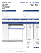 Purchase Order with Price List
See Dynamic Named Ranges in action. This template uses multiple customizable lists for selecting items descriptions, vendor and ship to addresses, and other options. The item description list uses the OFFSET formula and the other lists use the INDEX formula.
C) The INDIRECT Function
The INDIRECT function is another awesome function for creating dynamic ranges. It is also a volatile function, but like I mentioned above, that might not matter. The INDIRECT function lets you define a reference from a text string, and you can use concatenation to create the text string, like this:
=INDIRECT("Sheet1!A1:A"&row_num)
In the example shown at the top of this post, to create the reference «Sheet1!A2:A9» we replace row_num with MATCH(«zzz»,$A:$A) to return the row number of the last text value.
Important: When using INDIRECT to reference a range on a different worksheet, don’t forget to include the worksheet name in the string. When you enter a reference in the Refers To field via the Name Manager, Excel will automatically change $A:$A to «Sheet1!$A:$A» but it won’t know how to change your text string. This is one of the cons to using INDIRECT because if you change the name of the worksheet, you’ll need to remember to update your INDIRECT formula.
D) Structured References with Excel Tables
Beginning with Excel 2007, Microsoft introduced a new way to work with data in what are called Excel Tables, not to be confused with Data Tables, or other generic uses of the term table (yes, it is confusing).
If you use an official «Excel Table,» you can use a type of reference known as a structured reference. The structured reference uses the table name and the column labels like this:
=Table1[Categories]
You don’t need to know how to type the correct structured reference. While you are entering a formula, if you select the column in the Table, Excel will automatically change your reference to the structured reference.
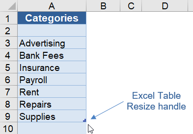
The reason these types of references can be considered dynamic is because of the unique way that table references behave when you expand or contract the table. Meaning, if you extend the table down by dragging the resize handle in the lower-right corner of the table, the reference =Table1[Categories] will automatically include the new rows.
So, instead of using an OFFSET formula to extend a range to the last value in a customizable list, we can let the user change the size of the list using the drag handle. Of course, this requires the user to know how to use Tables and the drag handle. That is one of the reasons I don’t often use this technique in my templates (that, and lack of compatibility with OpenOffice and Google Sheets).
E) The CHOOSE and IF Functions
Although I don’t use the CHOOSE function or nested IF formulas to create lists of variable length, they are pretty powerful functions for creating other types of dynamic ranges. For example, the two formulas below both return a different range (range_1, range_2 or range_3) based on a given number:
=CHOOSE(number,range_1,range_2,range_3,...)
=IF(number=1,range_1,IF(number=2,range_2,IF(number=3,range_3)))
The CHOOSE function is basically a shortcut for the nested IF formula in this case. When possible, I prefer using CHOOSE over nested IF formulas (if only to avoid having a million closing parentheses at the end of the formula ))))))))))).
See CHOOSE in action: My article «Create a Drop Down List in Excel» shows an example using CHOOSE to create a dependent drop down list.
Find the Position of the LAST Value in the Column
When using a dynamic named range for lists of variable length, we need to know how to find the numeric position of the last value in the column. In the examples above we used MATCH(«zzz»,range) for text values, but for numeric data or a combination of text and numeric data we may need to use something different. The formulas below cover all the scenarios I’ve come across.
The following image will be used for the example. It shows the reference and range and the position numbers of the values in the range.

1. Find the Position of the Last Numeric Value
The following formulas will allow the range to include blanks, error values, and text values, but the formulas will only return the position of the last numeric value. The result would be 4 in the example above.
=MATCH(1E+100,range,1)
=LOOKUP(42,1/ISNUMBER(range),ROW(range)-ROW(reference)+1)
See my article about VLOOKUP and INDEX-MATCH for a more detailed explanation of these MATCH and LOOKUP formulas. LOOKUP does not behave the same way in OpenOffice and Google Sheets. So, for maximum compatibility, I still prefer to use MATCH.
The value 9.99999999999999E+307 could be used for the MATCH function because it is the largest numeric value that can be stored in a cell, but that is kind of overkill. I prefer to use something more concise like 1E+100 or 10^100 (a googol).
2. Find the Position of the Last Text Value
The following formulas will allow the range to include blanks, error values, and numeric values, but the formulas will only return the position of the last text value (row 5 in the example above).
=MATCH("zzzz",range,1)
=LOOKUP(42,1/ISTEXT(range),ROW(range)-ROW(reference)+1)
Note: Using «zzzz» for the lookup value is not fool proof. The Greek, Cyrillic, Hebrew, and Arabic Unicode characters (and possibly other Unicode characters) come after z in the sort order. You might try using a high-value unicode symbol such as 🗿 if you expect the list to contain symbols.
3. Find the Position of the Last Non-Blank Value
When we want to return the last non-blank value, we can use the largest position returned by the two MATCH formulas listed above, or we can use the LOOKUP formula.
=MAX(MATCH(9E+307,range),MATCH("🗿",range))
=LOOKUP(42, 1/NOT(ISBLANK(range)), ROW(range)-ROW(reference)+1 )
Note that the empty string «» is not blank. It is treated as a text value.
A cell containing a formula is not blank, even if the formula returns an empty string. So, use the next method if you want to find the last non-empty value when you are using formulas that might return an empty string.
4. Find the Position of the Last Non-Empty Value «»
In many practical applications (like loan calculators), we may not necessarily want to find the last non-blank cell ( meaning no values or formulas), but instead may want to find the last non-empty cell.
If we define «empty» as the empty string «», then we can return the last non-empty value using the formula below. This might look like an array formula, but it isn’t, thanks to the way LOOKUP works (See this article on exceljet.net).
=LOOKUP(42, 1/(range<>""), ROW(range)-ROW(reference)+1 )
As I mentioned before, LOOKUP does not work the same way in OpenOffice and Google Sheets, but SUMPRODUCT provides a good solution.
=SUMPRODUCT(MAX((range<>"")*(ROW(range)-ROW(reference)+1)))
The SUMPRODUCT function allows you to avoid entering the formula as an array formula (not having to use Ctrl+Shift+Enter). Inside the SUMPRODUCT function, we are multiplying the boolean (FALSE=0 or TRUE=1) result for the (range<>»») comparison by the relative row number, so that the maximum result is the row number of the last blank cell.
Bonus: Create a Dynamic Print Area
When you create a print area in Excel via Page Layout > Print Area > Set Print Area, Excel actually creates a special named range called Print_Area. You can then go to Formulas > Name Manager and edit that named range to use a formula like this:
=OFFSET(start_cell,0,0,rows,columns)
This is a technique I use in some financial templates like the Home Mortgage Calculator to limit the print area based on the length of the payment schedule.
The catch: If you edit the Page Layout (margins, scaling, etc.), the Print_Area reference is changed to a regular reference. I’m not sure why the formula is removed, but this is basically a bug in Excel that has yet to be resolved. To avoid recreating the formula, I typically copy the formula and paste it into a text editor so that I can easily recreate the dynamic print area after I’m done making changes to the page layout.
No Dynamic Named Ranges in Google Sheets
Perhaps things will change in the future, but as of my last update (Sep 28, 2017), you cannot create named formulas using the Named Ranges feature in Google Sheets. This means that although you can use a Named Range for a drop-down list, you can’t create a Dynamic Named Range using a formula in Google Sheets.
Ben Collins shows how you can use a cell to create a text string like «A1:A»&row_num, name the cell, and then use INDIRECT(theName) to get some of the function of a dynamic named range. Unfortunately, that still doesn’t work for drop-down lists, because you can’t use INDIRECT(theCell) as the Range for a drop-down list.
References Related to Dynamic Named Ranges
- Dynamic Named Ranges at ozgrid.com — I think Dave Hawley’s site is the first place I saw the term «dynamic named range» used. Now, you can find articles on the subject at most Excel help sites.
- Using structured references with Excel tables at support.office.com
- Excel Named Ranges at contextures.com — A great article by Debra Dalgleish about how to create and use named ranges in Excel.