
Excel for Microsoft 365 Excel for Microsoft 365 for Mac Excel for the web Excel 2021 Excel 2021 for Mac Excel 2019 Excel 2016 Excel for iPad Excel for iPhone Excel for Android tablets Excel for Android phones More…Less
Excel formulas that return a set of values, also known as an array, return these values to neighboring cells. This behavior is called spilling.
Formulas that can return arrays of variable size are called dynamic array formulas. Formulas that are currently returning arrays that are successfully spilling can be referred to as spilled array formulas.
Following are some notes to help you understand and use these type of formulas.
What does spill mean?
Note: Older array formulas, known as legacy array formulas, always return a fixed-size result — they always spill into the same number of cells. The spilling behavior described in this topic does not apply to legacy array formulas.
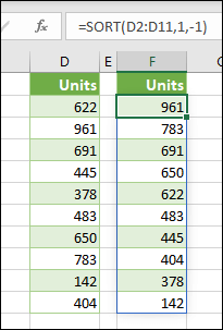
Spill means that a formula has resulted in multiple values, and those values have been placed in the neighboring cells. For example, =SORT(D2:D11,1,-1), which sorts an array in descending order, would return a corresponding array that’s 10 rows tall. But you only need to enter the formula in the top left cell, or F2 in this case, and it will automatically spill down to cell F11.
Key points
-
When you press Enter to confirm your formula, Excel will dynamically size the output range for you, and place the results into each cell within that range.
-
If you are writing a dynamic array formula to act on a list of data, it can be useful to place it in an Excel table, then use structured references to refer to the data. This is because structured references automatically adjust as rows are added or removed from the table.
-
Spilled array formulas are not supported in Excel tables themselves, so you should place them in the grid outside of the Table. Tables are best suited to holding rows and columns of independent data.
-
Once you enter a spilled array formula, when you select any cell within the spill area, Excel will place a highlighted border around the range. The border will disappear when you select a cell outside of the area.

-
Only the first cell in the spill area is editable. If you select another cell in the spill area, the formula will be visible in the formula bar, but the text is «ghosted», and can’t be changed. If you need to update the formula, you should select the top-left cell in the array range, change it as needed, then Excel will automatically update the rest of the spill area for you when you press Enter.
-
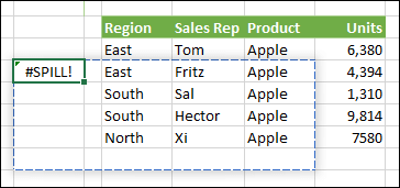
Formula overlap — Array formulas can’t be input if there is anything blocking the output range. and if this happens, Excel will return a #SPILL! error indicating that there is a blockage. If you remove the blockage, the formula will spill as expected. In the example below, the formula’s output range overlaps another range with data, and is shown with a dotted border overlapping cells with values indicating that it can’t spill. Remove the blocking data, or copy it somewhere else, and the formula will spill as expected.
-
Legacy array formulas entered via CTRL+SHIFT+ENTER (CSE) are still supported for back compatibility reasons, but should no longer be used. If you like, you can convert legacy array formulas to dynamic array formulas by locating the first cell in the array range, copy the text of the formula, delete the entire range of the legacy array, and then re-enter the formula in the top left cell. Before upgrading legacy array formulas to dynamic array formulas, you should be aware of some calculation differences between the two.
-
Excel has limited support for dynamic arrays between workbooks, and this scenario is only supported when both workbooks are open. If you close the source workbook, any linked dynamic array formulas will return a #REF! error when they are refreshed.

Need more help?
You can always ask an expert in the Excel Tech Community or get support in the Answers community.
See Also
FILTER function
RANDARRAY function
SEQUENCE function
SORT function
SORTBY function
UNIQUE function
#SPILL! errors in Excel
Implicit intersection operator: @
Need more help?
Что такое динамические массивы
В сентябре 2018 года Microsoft выпустила обновление, которое добавляет в Microsoft Excel совершенно новый инструменты: динамические массивы (Dynamic Arrays) и 7 новых функций для работы с ними. Эти вещи, без преувеличения, совершенно кардинальным образом меняет всю привычную технику работы с формулами и функциями и касаются, буквально, каждого пользователя.
Рассмотрим простой пример, чтобы объяснить суть.
Предположим, что у нас есть простая табличка с данными по городам-месяцам. Что будет если мы выделим любую пустую ячейку справа на листе и введем в нее формулу-ссылку не на одну ячейку, а сразу на диапазон?

Во всех прошлых версиях Excel после нажатия на Enter мы бы получили содержимое только одной первой ячейки B2. А как иначе?
Ну, или можно было бы завернуть этот диапазон в какую-нибудь аггрегирующую функцию типа =СУММ(B2:C4) и получить по нему общий итог.
Если бы нам потребовались операции посложнее примитивной суммы, например, извлечение уникальных значений или Топ-3, то пришлось бы вводить нашу формулу как формулу массива, используя сочетание клавиш Ctrl+Shift+Enter.
Теперь всё по-другому.
Теперь после ввода такой формулы мы можем просто нажать на Enter — и получить в результате сразу все значения, на которые мы ссылались:

Это не магия, а новые динамические массивы, которые теперь есть в Microsoft Excel. Добро пожаловать в новый мир 
Особенности работы с динамическими массивами
Технически, весь наш динамический массив хранится в первой ячейке G4, заполняя своими данными необходимое количество ячеек вправо и вниз. Если выделить любую другую ячейку массива, то в строке формул ссылка будет неактивной, показывая, что мы находимся в одной из «дочерних» ячеек:

Попытка удалить одну или несколько «дочерних» ячеек ни к чему не приведёт — Excel тут же заново их вычислит и заполнит.
При этом ссылаться на эти «дочерние» ячейки в других формулах мы можем совершенно спокойно:

Если копировать первую ячейку массива (например из G4 в F8), то и и весь массив (его ссылки) сдвинется в том же направлении, как и в обычных формулах:

Если нам нужно переместить массив, то достаточно будет перенести (мышью или сочетанием Ctrl+X, Ctrl+V), опять же, только первую главную ячейку G4 — вслед за ней перенесется на новое место и заново развернётся весь наш массив.
Если вам нужно сослаться где-нибудь еще на листе на созданный динамический массив, то можно использовать спецсимвол # («решётка») после адреса его ведущей ячейки:

Например, теперь можно легко сделать выпадающий список в ячейке, который ссылается на созданный динамический массив:

Ошибки динамических массивов
Но что будет, если для развёртывания массива не будет достаточно пространства или на его пути окажутся ячейки уже занятые другими данными? Знакомьтесь с принципиально новым типом ошибок в Excel — #ПЕРЕНОС! (#SPILL!):

Как всегда, если щелкнуть мышью по значку с желтым ромбом и восклицательным знаком, то мы получим более подробное пояснение по источнику проблемы и сможем быстро найти мешающие ячейки:

Аналогичные ошибки будут возникать, если массив выходит за пределы листа или натыкается на объединенную ячейку. Если удалить препятствие, то всё тут же исправится на лету.
Динамические массивы и «умные» таблицы
Если динамический массив указывает на «умную» таблицу, созданную сочетанием клавиш Ctrl+T или с помощью Главная — Форматировать как таблицу (Home — Format as Table), то он также унаследует её главное качество — автоподстройку размеров.

При добавлении новых данных внизу или справа «умная» таблица и динамический диапазон тоже будут автоматически растягиваться:

При этом, однако, есть одно ограничение: мы не можем использовать ссылку на динамический диапазон в форумулах внутри «умной» таблицы:

Динамические массивы и другие функции Excel
Хорошо, скажете вы. Всё это интересно и забавно. Не нужно, как раньше, вручную протягивать формулу со ссылкой на первую ячейку исходного диапазона вниз и вправо и всё такое. И всё?
Не совсем.
Динамические массивы — это не просто еще один инструмент в Excel. Теперь они внедрены в самое сердце (или мозг) Microsoft Excel — его вычислительный движок. А это значит что и другие, привычные нам формулы и функции Excel теперь тоже поддерживают работу с динамическими массивами. Давайте разберём несколько примеров, чтобы вы осознали всю глубину произошедших изменений.
Транспонирование
Чтобы транспонировать диапазон (обменять местами строки и столбцы) в Microsoft Excel всегда имелась встроенная функция ТРАНСП (TRANSPOSE). Однако, чтобы её использовать, вы должны были сначала правильно выделить диапазон для результатов (например, если на входе был диапазон 5х3, то вы должны были обязательно выделить 3×5), потом ввести функцию и нажать сочетание Ctrl+Shift+Enter, т.к. она умела работать только в режиме формул массива.
Теперь можно просто выделить одну ячейку, ввести в нее эту же формулу и нажать на обычный Enter — динамический массив сделает всё сам:

Таблица умножения
Этот пример я обычно приводил, когда меня просили наглядно показать преимущества формул массива в Excel. Теперь чтобы посчитать всю таблицу Пифагора достаточно встать в первую ячейку B2, ввести туда формулу перемножающую два массива (вертикальный и горизонтальный набор чисел 1..10) и просто нажать на Enter:

Склейка и преобразование регистра
Массивы можно не только перемножать, но склеивать стандартным оператором & (амперсанд). Предположим, нам нужно сцпеить имя и фамилию из двух столбцов и поправить скачущий регистр в исходных данных. Делаем это одной короткой формулой, которая формирует весь массив, а потом применяем к нему функцию ПРОПНАЧ (PROPER), чтобы привести в порядок регистр:

Вывод Топ-3
Предположим, что у нас есть куча чисел, из которых нужно вывести три лучших результата, расположив их в порядке убывания. Теперь это делается одной формулой и, опять же, без всяких Ctrl+Shift+Enter как раньше:

Если захочется, чтобы результаты располагались не в столбец, а в строку, то достаточно заменить в этой формуле двоеточия (разделитель строк) на точку с запятой (разделитель элементов внутри одной строки). В англоязычной версии Excel роль этих разделителей играют точка с запятой и запятая, соответственно.
ВПР извлекающая сразу несколько столбцов
Функцей ВПР (VLOOKUP) теперь можно вытаскивать значения не из одного, а сразу из нескольких столбцов — достаточно указать их номера (в любом желаемом порядке) в виде массива в третьем аргументе функции:

Функция СМЕЩ (OFFSET) возвращающая динамический массив
Одной из самых интересных и полезных (после ВПР) функций для анализа данных является функция СМЕЩ (OFFSET), которой я посвятил в своё время целую главу в своей книжке и статью здесь. Сложность в понимании и освоении этой функции всегда была в том, что она возвращала в качестве результата массив (диапазон) данных, но увидеть его мы не могли, т.к. Excel до сих пор не умел работать с массивами «из коробки».
Сейчас эта проблема в прошлом. Посмотрите, как теперь с помощью одной формулы и динамического массива, возвращаемого СМЕЩ, можно извлечь все строки по заданному товару из любой отсортированной таблицы:

Давайте разберём её аргументы:
- А1 — стартовая ячейка (точка отсчёта)
- ПОИСКПОЗ(F2;A2:A30;0) — вычисление сдвига от стартовой ячейки вниз — до первой найденной капусты.
- 0 — сдвиг «окна» вправо относительно стартовой ячейки
- СЧЁТЕСЛИ(A2:A30;F2) — вычисление высоты возвращаемого «окна» — количества строк, где есть капуста.
- 4 — размер «окна» по горизонтали, т.е. выводим 4 столбца
Новые функции для динамических массивов
Помимо поддержки механизма динамических массивов в старых функциях, в Microsoft Excel были добавлены несколько совершенно новых функций, заточенных именно под работу с динамическими массивами. В частности, это:
- СОРТ (SORT) — сортирует входной диапазон и выдает динамический массив на выходе
- СОРТПО (SORTBY) — умеет сортировать один диапазон по значениям из другого
- ФИЛЬТР (FILTER) — извлекает из исходного диапазона строки, удовлетворяющие заданным условиям
- УНИК (UNIQUE) — извлекает из диапазона уникальные значения или убирает повторы
- СЛМАССИВ (RANDARRAY) — генерит массив случайных чисел заданного размера
- ПОСЛЕД (SEQUENCE) — формирует массив из последовательности чисел с заданным шагом
Подробнее про них — чуть позже. Они стоят отдельной статьи (и не одной) для вдумчивого изучения
Выводы
Если вы прочитали всё написанное выше, то, думаю, уже осознаёте масштаб изменений, которые произошли. Очень многие вещи в Excel теперь можно будет делать проще, легче и логичнее. Я, признаться, немного в шоке от того, сколько статей теперь придется корректировать здесь, на этом сайте и в моих книгах, но готов это сделать с легким сердцем.
Подбивая итоги, в плюсы динамических массивов можно записать следующее:
- Можно забыть про сочетание Ctrl+Shift+Enter. Теперь Excel не видит различий между «обычными формулами» и «формулами массива» и обрабатывает их одинаково.
- Про функцию СУММПРОИЗВ (SUMPRODUCT), которую раньше использовали для ввода формул массива без Ctrl+Shift+Enter тоже можно забыть — теперь достаточно просто СУММ и Enter.
- Умные таблицы и привычные функции (СУММ, ЕСЛИ, ВПР, СУММЕСЛИМН и т.д.) теперь тоже полностью или частично поддерживают динамические массивы.
- Есть обратная совместимость: если открыть книгу с динамическими массивами в старой версии Excel, то они превратятся в формулы массива (в фигурных скобках) и продолжат работать в «старом стиле».
Нашлось и некоторое количество минусов:
- Нельзя удалить отдельные строки, столбцы или ячейки из динамического массива, т.е. он живёт как единый объект.
- Нельзя сортировать динамический массив привычным образом через Данные — Сортировка (Data — Sort). Для этого есть теперь специальная функция СОРТ (SORT).
- Динамический диапазон нельзя превратить в умную таблицу (но можно сделать динамический диапазона на основе умной таблицы).
Само-собой, это еще не конец и, я уверен, Microsoft продолжит совершенствовать этот механизм в будущем.
Где скачать?
И, наконец, главный вопрос
Microsoft впервые анонсировало и показало превью динамических массивов в Excel еще в сентябре 2018 года на конференции Ignite. В последующие несколько месяцев происходило тщательное тестирование и обкатка новых возможностей сначала на кошках сотрудниках самой Microsoft, а потом на добровольцах-тестировщиках из круга Office Insiders. В этом году обновление, добавляющее динамические массивы стали постепенно раскатывать уже по обычным подписчикам Office 365. Я, например, получил его только в августе с моей подпиской Office 365 Pro Plus (Monthly Targeted).
Если в вашем Excel ещё нет динамических массивов, а поработать с ними очень хочется, то есть следующие варианты:
- Если у вас подписка Office 365, то можно просто продождать, пока до вас дойдет это обновление. Как быстро это случится — зависит от настройки частоты доставки обновлений для вашего Office (раз в год, раз в полгода, раз в месяц). Если у вас корпоративный ПК, то можно попросить вашего администратора настроить загрузку обновлений почаще.
- Можно записаться в ряды тех самых добровольцев-тестировщиков Office Insiders — тогда вы будете первым получать все новые возможности и функции (но есть шанс повышенной глючности в работе Excel, само-собой).
- Если у вас не подписка, а коробочная standalone-версия Excel, то придется ждать до выхода следующей версии Office и Excel в 2022 году, как минимум. Пользователи таких версий получают только обновления безопасности и исправления ошибок, а все новые «плюшки» теперь достаются только подписчикам Office 365. Sad but true
В любом случае, когда динамические массивы появятся в вашем Excel — после этой статьи вы будете к этому уже готовы
Ссылки по теме
- Что такое формулы массива и как их использовать в Excel
- Суммирование по окну (диапазону) с помощью функции СМЕЩ (OFFSET)
- 3 способа транспонировать таблицу в Excel
The key benefit of Dynamic Arrays is the ability to work with multiple values at the same time in a formula. This is a big upgrade and welcome change. Dynamic Arrays solve some really hard problems in Excel, and will fundamentally change the way worksheets are designed. Once you see how they work, you’ll never want to go back.
Availability
Dynamic arrays and the new functions below are only available Excel 365 and Excel 2021. Excel 2019 and earlier do not offer dynamic array formulas. For convenience, I’ll use «Dynamic Excel» (Excel 365) and «Legacy Excel» (2019 or earlier) to differentiate versions below.
New functions
As part of the dynamic array update, Excel now includes 8 new functions which directly leverage dynamic arrays to solve problems that are traditionally hard to solve with conventional formulas. Click the links below for details and examples for each function:
| Function | Purpose |
|---|---|
| FILTER | Filter data and return matching records |
| RANDARRAY | Generate array of random numbers |
| SEQUENCE | Generate array of sequential numbers |
| SORT | Sort range by column |
| SORTBY | Sort range by another range or array |
| UNIQUE | Extract unique values from a list or range |
| XLOOKUP | Modern replacement for VLOOKUP |
| XMATCH | Modern replacement for the MATCH function |
Video: New dynamic array functions in Excel (about 3 minutes).
As of January 2023, many more new functions have now been released to take advantage of the dynamic array engine. The complete list of new functions is: ARRAYTOTEXT, BYCOL, BYROW, CHOOSECOLS, CHOOSEROWS, DROP, EXPAND, FILTER, HSTACK, ISOMITTED, LAMBDA, LET, MAKEARRAY, MAP, RANDARRAY, REDUCE, SCAN, SEQUENCE, SORT, SORTBY, STOCKHISTORY, TAKE, TEXTAFTER, TEXTBEFORE, TEXTSPLIT, TOCOL, TOROW, UNIQUE, VALUETOTEXT, VSTACK, WRAPCOLS, WRAPROWS, XLOOKUP, and XMATCH.
Example
Before we get into the details, let’s look at a simple example. Below we are using the new UNIQUE function to extract unique values from the range B5:B15, with a single formula entered in E5:
=UNIQUE(B5:B15) // return unique values in B5:B15

The result is a list of the five unique city names, which appear in E5:E9.
Like all formulas, UNIQUE will update automatically when data changes. Below, Vancouver has replaced Portland on row 11. The result from UNIQUE now includes Vancouver:

Spilling — one formula, many values
In Dynamic Excel, formulas that return multiple values will «spill» these values directly onto the worksheet. This will immediately be more logical to formula users. It is also a fully dynamic behavior – when source data changes, spilled results will immediately update.
The rectangle that encloses the values is called the «spill range». You will notice that the spill range has special highlighting. In the UNIQUE example above, the spill range is E5:E10.
When data changes, the spill range will expand or contract as needed. You might see new values added, or existing values disappear. In this way, a spill range is a new kind of dynamic range.
In Legacy Excel, by contrast, you can see multiple results returned by array formula in the formula bar if you use F9 to inspect the formula. However, unless the formula is entered as a multi-cell array formula, only one value will display on the worksheet. This behavior has always made array formulas difficult to understand. Spilling makes array formulas more intuitive.
Note: when spilling is blocked by other data, you’ll see a #SPILL error. Once you make room for the spill range, the formula will automatically spill.
Video: Spilling and the spill range
Spill range reference
To refer to a spill range, use a hash symbol (#) after the first cell in the range. For example, to reference the results from the UNIQUE function above use:
=E5# // reference UNIQUE results
This is the same as referencing the entire spill range, and you’ll see this syntax when you write a formula that refers to a complete spill range.
You can feed a spill range reference into other formulas directly. For example, to count the number of cities returned by UNIQUE, you can use:
=COUNTA(E5#) // count unique cities

When the spill range changes, the formula will reflect the latest data.
Massive simplification
The addition of new dynamic array formulas means certain formulas can be drastically simplified. Here are a few examples:
- Extract and list unique values (before | after)
- Count unique values (before | after)
- Filter and extract records (before | after)
- Extract partial matches (before | after)
The power of one
One of the most powerful benefits of the «one formula, many values» approach is less reliance on absolute or mixed references. As a dynamic array formula spills results onto the worksheet, references remain unchanged, but the formula generates correct results.
For example, below we use the FILTER function to extract records in group «A». In cell F5, a single formula is entered:
=FILTER(B5:D11,B5:B11="a") // references are relative

Notice both ranges are unlocked relative references, but the formula works perfectly.
This is a huge benefit for many users, because it makes the process of writing formulas so much simpler. For another good example, see the multiplication table below.
Chaining functions
Things get really interesting when you chain together more than one dynamic array function. Perhaps you want to sort the results returned by UNIQUE? Easy. Just wrap the SORT function around the UNIQUE function like this:

As before, when source data changes, new unique results automatically appear, nicely sorted.
Native behavior
It’s important to understand that dynamic array behavior is a native and deeply integrated. When any formula returns multiple results, these results will spill into multiple cells on the worksheet. This includes older functions not originally designed to work with dynamic arrays.
For example, in Legacy Excel, if we give the LEN function a range of text values, we’ll see a single result. In Dynamic Excel, if we give the LEN function a range of values, we’ll see multiple results. This screen below shows the old behavior on the left and the new behavior on the right:

This is a huge change that can affect all kinds of formulas. For instance, the VLOOKUP function is designed to fetch a single value from a table, using a column index. However, in Dynamic Excel, if we give VLOOKUP more than one column index using an array constant like this:
=VLOOKUP("jose",F7:H10,{1,2,3},0)
VLOOKUP will return multiple columns:

In other words, even though VLOOKUP was never designed to return multiple values, it can now do so, thanks to the new formula engine in Dynamic Excel.
All formulas
Finally, note that dynamic arrays work with all formulas not just functions. In the example below cell C5 contains a single formula:
=B5:B14*C4:L4
The result spills into a 10 by 10 range that includes 100 cells:

If the numbers in the ranges B5:B14 and C4:L4 where are themselves dynamic arrays (i.e. created with the SEQUENCE function), the spill reference operator can be used like this:
=B5#*C4# // returns same 10 x 10 array
Arrays go mainstream
With the rollout of dynamic arrays, the word «array» is going to pop up much more often. In fact, you may see «array» and «range» used almost interchangeably. You’ll see arrays in Excel enclosed in curly braces like this:
{1,2,3} // horizontal array
{1;2;3} // vertical array
Array is a programming term that refers to a list of items that appear in a particular order. The reason arrays come up so often in Excel formulas is that arrays can perfectly express the values in a range of cells.
Video: What is an array?
Array operations become important
Because Dynamic Excel formulas can easily work with multiple values, array operations will become more important. The term «array operation» refers to an expression that runs a logical test or math operation on an array. For example, the expression below tests if values in B5:B9 are equal to «ca»
=B5:B9="ca" // state = "ca"

because there are 5 cells in B5:B9, the result is 5 TRUE/FALSE values in an array:
{FALSE;TRUE;FALSE;TRUE;TRUE}
The array operation below checks for amounts greater than 100:
=C5:C9>100 // amounts > 100

The final array operation combines test A and test B in a single expression:
=(B5:B9="ca")*(C5:C9>100) // state = "ca" and amount > 100

Note: Excel automatically coerces the TRUE and FALSE values to 1 and 0 during the math operation.
To bring this back to dynamic array formulas in Excel, the example below demonstrates how we can use exactly the same array operation inside the FILTER function as the include argument:

FILTER returns the two records where state = «ca» and amount > 100.
For a demonstration, see: How to filter with two criteria (video).
New and old array formulas
In Dynamic Excel, there is no need to enter array formulas with control + shift + enter. When a formula is created, Excel checks if the formula might return multiple values. If so, it will automatically be saved as a dynamic array formula, but you will not see curly braces. The example below shows a typical array formula entered in Dynamic Excel:

If you open the same formula in Legacy Excel, you’ll see curly braces:

Going the other direction, when a «traditional» array formula is opened in Dynamic Excel, you will see the curly braces in the formula bar. For example, the screen below shows a simple array formula in Legacy Excel:

However, if you re-enter the formula with no changes, the curly braces are removed, and the formula returns the same result:

The bottom line is that array formulas entered with control + shift + enter (CSE) still work to maintain compatibility, but you shouldn’t need to enter array formulas with CSE in Dynamic Excel.
The @ character
With the introduction of dynamic arrays, you’re going to see the @ character appear more often in formulas. The @ character enables a behavior known as «implicit intersection». Implicit intersection is a logical process where many values are reduced to one value.
In Legacy Excel, implicit intersection is a silent behavior used (when necessary) to reduce multiple values to a single result in one cell. In Dynamic Excel, it is not typically needed, since multiple results can spill onto the worksheet. When it is needed, implicit intersection is invoked manually with the @ character.
When opening spreadsheets created in an older version of Excel, you may see the @ character added automatically to existing formulas that have the potential to return many values. In Legacy Excel, a formula that returns multiple values won’t spill on the worksheet. The @ character forces this same behavior in Dynamic Excel so that the formula behaves the same way and returns the same result as it did in the original Excel version.
In other words, the @ is added to prevent an older formula from spilling multiple results onto the worksheet. Depending on the formula, you may be able to remove the @ character and the behavior of the formula will not change.
Summary
- Dynamic Arrays will make certain formulas much easier to write.
- You can now filter matching data, sort, and extract unique values easily with formulas.
- Dynamic Array formulas can be chained (nested) to do things like filter and sort.
- Formulas that return more than one value will automatically spill.
- It is not necessary to use Ctrl+Shift+Enter to enter an array formula.
- Dynamic array formulas are only available in Excel 365.
Excel has changed… like seriously, changed. Every time we used Excel in the past, we accepted a simple operating rule; one formula one cell. Even with advanced formulas, it was still necessary to have a cell for each. But this has changed; Excel now allows a single formula to fill multiple cells. This is possible because Microsoft has changed Excel’s calculation engine to allow dynamic arrays.
The term dynamic arrays sounds complicated, but once you understand it, you’ll appreciate its simplicity and power.
Note: At the time of writing, dynamic arrays are available in Excel 365, Excel Online and Excel 2021 only. Excel 2019 and prior will not be updated to include dynamic arrays.
Watch the video:
Watch the video on YouTube
Overview of dynamic arrays
Let’s begin by looking at a basic example. Here is the formula:
=B2:B6OK, it’s not a formula you’ve ever used, but it’s simple enough to help describe the impact of dynamic arrays.
Before dynamic arrays
In Excel 2019 and prior, only one cell result could be returned by a formula. If we provided a formula with five results (cell B2, B3, B4, B5, and B6, as per our example), then some assumptions needed to be made by Excel. As a result, there are multiple outcomes from the formula above:
- If the formula was in line with the source data Excel assumed we want the value from the same row.
- If the formula was not in line with the source data, Excel got confused and returned the #VALUE! error.
Take a look at the screenshot below:
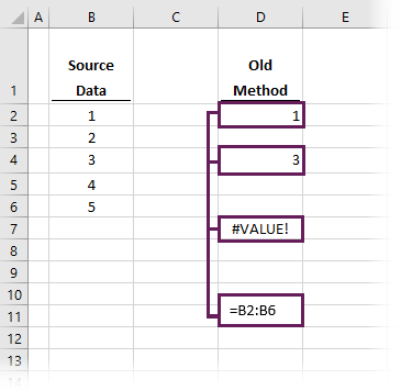
The value of 1 is shown in cell D2, as Excel assumes we want the value from cell B2 because it is in line with it. Had we entered exactly that same formula in cell D4, Excel assumes we want the inline cell, so returns 3 from cell B4.
Since cell D7 is not in line with any of the source data, Excel doesn’t know what we want, and returns the #VALUE! error. This assumption has got a technical name, implicit intersection. But we don’t really need to worry about that anymore.
It’s interesting to think that Excel could calculate different results from the same formula (hopefully a thing of the past). To override implicit intersection, Excel allowed us to press Ctrl+Shift+Enter when entering formulas. But we don’t need to worry about that anymore either.
With dynamic arrays
If we have a newer, dynamic array enabled version of Excel, there is only one possible result for our example formula; Excel returns all 5 cells. In the screenshot below, cell D2 contains the formula, but the result is shown in cells D2, D3, D4, D5 and D6. One formula displays 5 results… amazing!
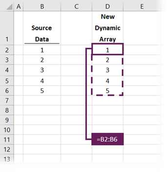
The basic rule of one formula one cell has gone. The terminology to describe a formula filling multiple cells is spilling, and the range of cells filled by that formula is called the spill range.
Which versions of Excel have dynamic arrays?
Microsoft originally announced the change to Excel’s calculation engine in September 2018. For over a year, it was only available to those who signed up to test early releases of the new features. Regular subscribers on the Microsoft 365 monthly update channel started to receive the update from November 2019. Finally, in July 2020, those on the semi-annual channel of the Microsoft 365 subscription (mostly business users) also received dynamic arrays.
Microsoft has already confirmed this new functionality will not be available in Excel 2019 or prior versions. So, if you want it, then it’s time to upgrade to Excel 2021 or a Microsoft 365 license.
New dynamic array functions
When Microsoft announced the new dynamic array functionality, they also introduced 6 new functions. All of which make use of this new calculation engine:
- UNIQUE – to list the unique or distinct values in a range
- SORT – to sort the values in a range
- SORTBY – to sort values based on the order of other values
- FILTER – to return only the values which meet specific criteria
- SEQUENCE – to return a sequence of numbers
- RANDARRAY – to return an array of random numbers
While we all get excited by new functions, the introduction of dynamic arrays is bigger than this; it’s a fundamental shift in how Excel (and Excel users) think about ALL formulas. In the remainder of this post, you get to understand the basics needed to start thinking in this new way.
Dynamic array formulas
As noted above, there are new functions that make use of this new spilling functionality. We won’t go into detail about each of these in this post; there are separate posts for each of them. The critical thing to realize is that the ability to spill is not restricted to these new functions; many existing functions now spill too.
Look at the example data below.
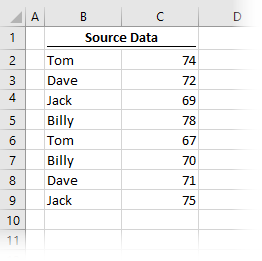
This is a simple scenario in which we have data in cells B2-C9. This data displays a name and a score. Let’s assume the goal is to calculate the total score for each person.
Before dynamic arrays
To calculate the total score for each individual, we could use the SUMIFS function.
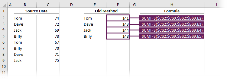
Cells F2-F5 each contain a formula. For example, F2 contains the following:
=SUMIFS($C$2:$C$9,$B$2:$B$9,E2)To calculate the result for each person, this formula would be copied down into the 3 rows below. In each formula, the last argument would change to reference cells E3, E4 and E5, respectively.
With dynamic arrays
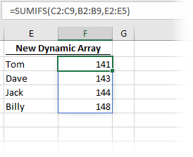
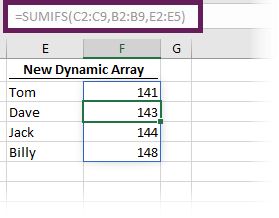
But wait, the new Excel calculation engine returns multiple results from a single formula. Much like how our basic formula at the beginning of the post pushed results into other cells, SUMIFS works the same.
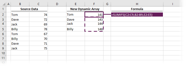
Rather than having 4 formulas, one for each cell; we can have one formula which returns results into 4 cells. The formula in cell F2 demonstrates this:
=SUMIFS(C2:C9,B2:B9,E2:E5)The last argument in the SUMIFS function is the value to be matched. Rather than one value, we provided an array of values to match in cells E2-E5. Therefore, Excel has performed all 4 calculations and spilled the results into cells F2-F5.
Which formulas spill?
So, which formulas spill, and which don’t? Good question. It depends on the arguments that the formula expects.
Basic aggregation functions, such as SUM, AVERAGE, MIN, MAX, etc., will not spill by themselves, which makes sense as they accept a range of values and only ever return a single value.
Generally, any function containing an argument in which a single value is evaluated expected is likely to spill. That single value has a technical term, it’s known as a scalar.
Let’s take VLOOKUP as an example. The first argument in VLOOKUP is the value to lookup, it’s generally a single value (it is a scalar). If we provide two or more values in that argument, the formula will spill, and calculate the result for each item included within the lookup value.
Look at the example below. The VLOOKUP in cell F7 is looking up Dave and Jack, so it calculates twice and returns the values in F7 and F8.
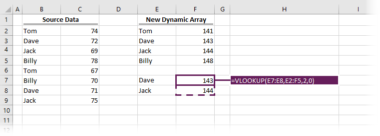
Generally, the rule is that If we’re working with standard formulas, then any time we use multiple scalars, it will spill. There are a few technical scenarios where this isn’t true, but that is outside the scope of this post.
Spilling
By clicking a formula or any cell in the spill range, a blue box is displayed to outline all the cells within the same spill range. Everything within the blue box is calculated by the top-left cell of that box.
By selecting any cell within the spill range, the formula bar displays the formula driving that result. If it is the top-left cell, we can edit the formula. However, if we select a cell, other than the top-left, the formula is greyed out and can’t be edited.
Look at the screenshot below; we have selected the second cell in the spill range. The formula is greyed out because it isn’t really in that cell, it’s in the top-left cell.
What happens if there is data already in the spill range? Will it overwrite the existing data? Thankfully, nothing too dramatic happens. Instead, the top-left cell returns a #SPILL! error.
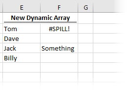
By clicking on the #SPILL! error, Excel displays a dotted line showing the spill range, and we can see what is causing the problem.
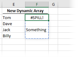
Then it’s your choice to (a) enter the formula in another location, or (b) move or delete the value causing the #SPILL! error.
#SPILL! errors occur in the following situations:
- The spill range is outside the available cells on the worksheet
- The spill range has an unknown size
- The dynamic array formula is included in an Excel table
- The spill range contains a merged cell
- The spill range is so large that Excel has run out of memory
# References
As a formula can spill results into other cells, we need a way to reference all the cells in the spill range. Thankfully, Microsoft has already thought of this and has created a new referencing methodology using the # symbol.
If the top-left cell in the spill range is in cell F2, we could reference the entire spill range by using F2#.
The screenshot below revisits our earlier example, but with an AVERAGE function added in cell F7.
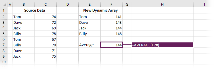
The formula in cell F7 is:
=AVERAGE(F2#)By using F2#, we are referencing all the cells in the spill range (cells F2, F3, F4 and F5). One significant advantage is that if the spill range changes size, the AVERAGE will automatically expand to include the increased range.
Constant arrays
Constant arrays have always existed in Excel; however, given the introduction of dynamic arrays, the use of constant arrays is likely to increase. They sound more complicated than they are. So, let’s just spend a few minutes understanding how they work.
The easiest way to understand this is with an example; let’s use VLOOKUP.
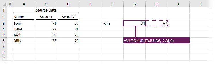
The formula in cell G3 is:
=VLOOKUP(F6,B2:D5,{2,3},0)This formula includes a constant array of {2,3}. Excel is using both values of 2 and 3 and spilling calculations for both into cell G3 and H3. The old method would require two formulas to achieve this, but with dynamic arrays we can use just one.
The two numbers in curly brackets are known as a constant array. See, they are not too scary after all.
With constant arrays, just be aware that columns are separated by commas and rows are separated by semi-colons. If we wanted to spill in rows instead of columns, we would use a semi-colon between the values (e.g., {2;3}).
=VLOOKUP(F6,B2:D5,{2;3},0)
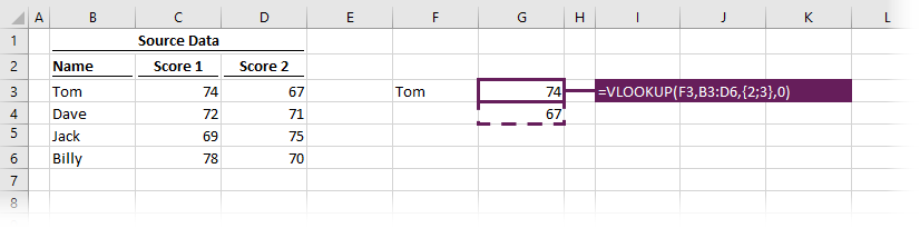
If we were to enter the 2 and 3 in the opposite order (e.g. {3,2}), then the values returned would switch order too.
The @ symbol
To force Excel to operate in the old way, we can use the @ symbol. Let’s head back to our original example:
=B2:B6To use the old implicit intersection method which only returns the values that are in the same row, we can add the @ symbol.
[email protected]:B6It’s unlikely that we would ever want to revert to the old way of calculating formulas. But initially, we are likely to see a lot of the @ symbol.
To ensure formulas built in previous versions of Excel continue to calculate the same result, the @ symbol will be added to some formulas automatically. This means that workbooks created in older versions of Excel but opened in the newer version of Excel should never spill. The @ symbol ensures backward compatibility.
NOTE: It may seem confusing because the @ symbol is already used within the structured referencing format that we use with Tables. But, if you think about it, in Tables, the @ symbol is used to reference items in the same row. Therefore, structured references in tables already have implicit intersection built in.
Conclusion
I’m sure you’ve got 100 questions spinning around your mind about dynamic arrays. There is a lot of new terminology and ways of working here. While the changes may seem confusing initially, you will soon see that this brings new powers to Excel users, which makes Excel easier to use.
Want to learn more?
There is a lot to learn about dynamic arrays and the new functions. Check out my other posts here to learn more:
- Introduction to dynamic arrays – learn how the excel calculation engine has changed.
- UNIQUE – to list the unique values in a range
- SORT – to sort the values in a range
- SORTBY – to sort values based on the order of other values
- FILTER – to return only the values which meet specific criteria
- SEQUENCE – to return a sequence of numbers
- RANDARRAY – to return an array of random numbers
- Using dynamic arrays with other Excel features – learn to use dynamic arrays with charts, PivotTables, pictures etc.
- Advanced dynamic array formula techniques – learn the advanced techniques for managing dynamic arrays

About the author
Hey, I’m Mark, and I run Excel Off The Grid.
My parents tell me that at the age of 7 I declared I was going to become a qualified accountant. I was either psychic or had no imagination, as that is exactly what happened. However, it wasn’t until I was 35 that my journey really began.
In 2015, I started a new job, for which I was regularly working after 10pm. As a result, I rarely saw my children during the week. So, I started searching for the secrets to automating Excel. I discovered that by building a small number of simple tools, I could combine them together in different ways to automate nearly all my regular tasks. This meant I could work less hours (and I got pay raises!). Today, I teach these techniques to other professionals in our training program so they too can spend less time at work (and more time with their children and doing the things they love).
Do you need help adapting this post to your needs?
I’m guessing the examples in this post don’t exactly match your situation. We all use Excel differently, so it’s impossible to write a post that will meet everybody’s needs. By taking the time to understand the techniques and principles in this post (and elsewhere on this site), you should be able to adapt it to your needs.
But, if you’re still struggling you should:
- Read other blogs, or watch YouTube videos on the same topic. You will benefit much more by discovering your own solutions.
- Ask the ‘Excel Ninja’ in your office. It’s amazing what things other people know.
- Ask a question in a forum like Mr Excel, or the Microsoft Answers Community. Remember, the people on these forums are generally giving their time for free. So take care to craft your question, make sure it’s clear and concise. List all the things you’ve tried, and provide screenshots, code segments and example workbooks.
- Use Excel Rescue, who are my consultancy partner. They help by providing solutions to smaller Excel problems.
What next?
Don’t go yet, there is plenty more to learn on Excel Off The Grid. Check out the latest posts:
Excel Dynamic Arrays – changing how Excel works
Many years ago, I heard Excel referred to as ‘Hell in a Cell’. I don’t know who coined this statement, but I have used it many times myself. In one cell you can only have 1 value. For every value, you need to enter either that value, or a formula to return a value. And each formula will return only one value. And that’s the way Excel works. Or that’s the way Excel did work.
Dynamic Arrays and Spill areas. Excel is moving from hell in a cell, to a whole new way of calculating. The entire calculation grid is changing how it works. It is becoming more powerful, faster and less prone to error. Now you will be able to create one formula and return many values.
Along with Dynamic Arrays and Spill areas are 6 new functions. FILTER, RANDARRAY, SQEUENCE, SORT, SORTBY and UNIQUE. But dynamic arrays are not limited to these new functions.
The possibilities are now endless. The way we work in Excel is about to change dramatically. Traditional Array functions entered using Ctrl + Shift + Enter to get those curly brackets are no longer for advanced users. CTRL + Shift + Enter is gone, along with the brackets. Excel will think in arrays and expect to return multiple values instead of one.
Dynamic Arrays Example 1 – Creating a Unique List
Consider the following table of sales data, although small, it is perfect for our example.

Suppose you need a unique list of Products. Under the old Excel it was a bit of a headache. You can do this this a number of ways depended on your needs and knowledge. You could write a complex formula. Or, you could load the data into Power Query, or you could use Advanced Filter.
Advanced Filter is okay if you are working with static data. If your column changes, you would have to re-run advanced filter to get a new unique list. I have often seen this method used by less experienced excel users. Then they wonder why things like data validation break!

There are just too many steps when using Power Query for the sole purpose of extracting a unique list. And if you were to use a formula, it would be a complex array formula. Way beyond the ability of most Excel users.
However, with Excels new array thinking and the new UNIQUE function, obtaining unique list is simple.
UNIQUE Function in Excel
The syntax for UNIQUE is
=UNIQUE(array, [by_col], [occurs_once])
We will explore the full detail of the UNIQUE function at a later stage. But as we know parameters in excel functions surrounded with square brackets [ ] can often be left out as they are optional.
Therefore, to get a unique list of the Products, the only parameter we need to feed the UNIQUE function is the array.
By using the formula =UNIQUE(sales[Products]) in only one cell, we can get a unique list.

As we entered an array, Excel knows to return an array, or more than one value. On hitting Enter, not only will the cell with the formula return a value, but the unique list will Spill down to other cells.

Recognizing and Working with Excel Dynamic Arrays
You will note from our UNIQUE example, 5 items were returned and these filled the column down. We did not enter formulas into the other cells. The range in which the function fills is known as the Spill range. By selecting any of the cells in the Spill range, a blue box will appear allowing you identify the entire spill range.
You will see the formulas in grey throughout the Spill range. You can not edit the formula in any of the Spill cells. It can only be edited in the cell in which it was entered.
If you have values in the Spill Range, you will get a Spill error. By selecting the cell with the error, a blue dotted line will show you where the Spill range wants to fill.

By clicking on the Formula warning, you can quickly select all obstruction cells, and delete, or move the data somewhere else.

Once you have cleared the area Excel wants to fill to, the error will be fixed and the results will spill.

This spill range is also dynamic. In our example we have the source data stored in table format. Hence the formula UNIQUE(sales[Products]) and not UNIQUE(B2:B18). If we now update this table with a new row of data, and a new product, the UNIQUE function also updates, and the Spill range expands.

Are you starting to see the benefits of the new calculation engine in Excel? By entering a formula only once, you are saving a lot of time, and you are less prone to error. More efficient and accurate. How cool is that. But wait, there is more, loads more.
Referencing values from Spill Ranges
You can use values from a Spill Range as an input to other formulas or features.
To reference ALL the values contained within a dynamic array, reference only the cell with the formula and then add # to the end. You can also reference the values from each cell within the spill range, by selecting just that cell.
For Example, we can use the function LEN to get the number of characters in each word. In this example = LEN(H4) we have referenced the actual cells reference H4. We can see the number of characters returned is correct at 5. The driving cell, H4, does not ‘really’ contain any values, as it is part of a spill range. If we copy this formula down, it works just like any Excel formula referencing a value from within a cell.

You can reference the entire Spill Range by adding the symbol # to the end of the cell reference that contains the dynamic array formula. For example, as per the image, in cell J2 is =LEN(H2#). Once we add the # the Dynamic array spill will be selected. The result is a spill showing the LEN of each value in our unique list.

The Spill in this case is 6 values. In old Excel, we would need 6 formulas entered into Excel to return these 6 values. We did not need to fill down the formula and we did not need to press CTRL+Shift+Enter for Excel to return an array.
Dynamic Arrays Example 2 – Dynamic Data Validation and SORT
With Dynamic Spill ranges, Excels Sort and Filter options do not work. Therefore, Microsoft have introduced new functions to help with this. SORT and FILTER functions.
We will look at both function in more detail at a different time. For now, we are going to take a quick look at SORT, so we can create a Sorted unique list to be use in a Data Validation drop down.
The syntax for sort is
SORT(array, [sort index], [sort order], [by col])
However we know the items in [ ] can be omitted. The default sort order in the SORT function is Ascending order. So, to sort our unique list A-Z we only need to enter the array to the function.
As the UNIQUE function returns an Array, we can use this array in our SORT function. =SORT(UNIQUE(sales[Product])) will therefore return a sorted unique list of our products.

We can then use this list to create a Dynamic Data validation drop down. You will find Data validation on the Data Ribbon.

In the data validation window, select Allow List. In the Source reference only the cell that contains the formula, in this case $H2$. We then add # to the end of the cell reference to tell Excel is it the Spill array that you want.

This will then create a dynamic drop down. The drop down will update as the unique list updates making it dynamic at all times.

Dynamic Arrays Example 3 – Transporting a Unique List
We have seen how a function spills down when we select a column. If we take a Row of values as our array, the spill will also go across the row. However, what if you needed values from a column to spill over a row? How would you go about this?
Well we can simply wrap our UNIQUE function between the TRANSPOSE function. The TRANSPOSE function is a old array formula that existed in Excel. Its syntax is
=TRANSPOSE(array)
We know our UNIQUE function returns an array. and if we had this UNIQUE wrapped in SORT, we would also have an array. Now we can just wrap TRANSPOSE around this.
For this example we will take a unique list of the Sales Rep.
=TRANSPOSE(SORT(UNIQUE(sales[Sales Rep])))

Dynamic Arrays Example 4 – 3 Formulas, 1 pivot table.
Did you every think you could create a calculation table like a pivot table using formulas. With Dynamic arrays, this becomes very simple.
Using only 2 formulas we have been able to create a column containing unique products and a row containing unique Sales Reps.

Now with only 1 more formula, we can get the total Value for each product by each Sales rep. Something most of us would only have considered calculating using a pivot table.
In cell I2 we are going to create a SUMIFS function. If you are not familiar with SUMIFS in Excel you can read this article here .
SUMIFS will allow you sum by multiple criteria. In our table, we have both Products and Sales Rep and we want to sum the VALUE for each
The syntax for SUMIFS is
=SUMIFS(Sum Range, Criteria Range 1, Criteria 1, [Criteria range 2, Criteria 2)….).
The formula we will use is
=SUMIFS(sales[Value],sales[Product],$H$2#,sales[Sales Rep],$I$1#)
The Sum range sales[Value] is the value we want to sum
Criteria range is the range where you will find the criteria defining what you want to sum. This is case we want to sum the Sales value, first based on the Sales[Product].
Next we define the first criteria we want to sum by. H2 contains Apples. However, we don’t just want Apples, we want all of the array. So, we use the # after the cell reference $H2$#.
The SUMIFS function then moves on to the second criteria. Taking the Sales Rep column, filter to the sales rep shown in the Spill array and then sum the values.

As we have taken the Spill ranges in our SUMIFS formula, the values returned for this formula will also spill.
Benefits Over Pivot tables
Creating a calculation table like this with only 3 formulas is very much a game changer. Before, if we created such a table using Excel Pivot Table features, the Pivot table would need a Refresh when source data table is updated.
However, with the user of Dynamic Arrays, there is no need to refresh as these arrays are truly dynamic and will update for you when you update your table.

As you can see this is fast, it is reliable, and it is less prone to human error. You do not have to remember to refresh and you don’t have to update any formulas. In addition, it also took only 3 formulas to create.
Backward Compatibility
The 6 new functions that arrive with Dynamic Arrays are not backward compatible. Neither is the spill range operator. However, if you open an Excel workbook in an earlier version, the values will remain intact and you can use these values in other formulas. But once you try edit the formula, it will break. You will note these formulas as in the formula bar you will see _xlfn, which indicates the formula is not supported.
When you open a workbook containing Dynamic Arrays in an older version, Excel will convert these to its only array structure. These will include the curly brackets and if you edit these formulas remember to press CTRL+Shift+Enter.
Conclusion
This new calculation engine and Excel Dynamic Arrays are only available in Excel 365 (currently insiders edition only). I have to say these changes are really amazing and they will completely change how I go about creating spreadsheets and models moving forward.
In this article we looked at only a few small examples. And we did not take a deep dive into any of the new functions. Instead I tried to select a few examples that would first show you how Dynamic Arrays work. And the show you some of the capabilities available when you use Dynamic Arrays with existing functions such as SUMIFS.