Duplicates values in excel

Sometimes duplicate data is useful, sometimes it just makes it harder to understand your data. Use conditional formatting to find and highlight duplicate data. That way you can review the duplicates and decide if you want to remove them.

1. Select the cells you want to check for duplicates.

   Note: Excel can’t highlight duplicates in the Values area of a PivotTable report.

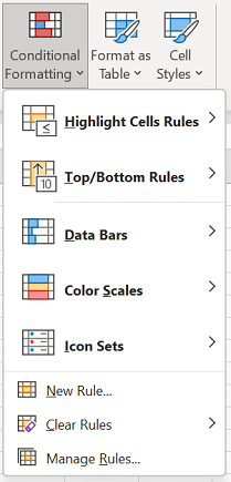
2. Click Home > Conditional Formatting > Highlight Cells Rules > Duplicate Values.

   

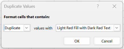
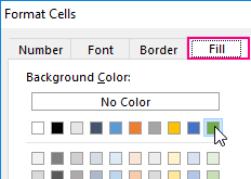
3. In the box next to values with, pick the formatting you want to apply to the duplicate values, and then click OK.

   ​​​​​​​

Remove duplicate values

When you use the Remove Duplicates feature, the duplicate data will be permanently deleted. Before you delete the duplicates, it’s a good idea to copy the original data to another worksheet so you don’t accidentally lose any information.

1. Select the range of cells that has duplicate values you want to remove.

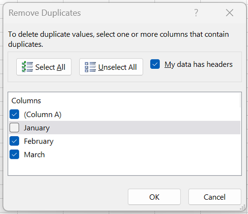
2. Click Data > Remove Duplicates, and then Under Columns, check or uncheck the columns where you want to remove the duplicates.

   

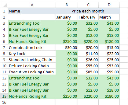
   For example, in this worksheet, the January column has price information I want to keep.

   

   So, I unchecked January in the Remove Duplicates box.

   

3. Click OK.

Note: The counts of duplicate and unique values given after removal may include empty cells, spaces, etc. 

Need more help?

​​​​​​​

Duplicate Values | Triplicates | Duplicate Rows

This example teaches you how to find duplicate values (or triplicates) and how to find duplicate rows in Excel.

Duplicate Values

To find and highlight duplicate values in Excel, execute the following steps.

1. Select the range A1:C10.

2. On the Home tab, in the Styles group, click Conditional Formatting.

3. Click Highlight Cells Rules, Duplicate Values.

4. Select a formatting style and click OK.

Result. Excel highlights the duplicate names.

Note: select Unique from the first drop-down list to highlight the unique names.

Triplicates

By default, Excel highlights duplicates (Juliet, Delta), triplicates (Sierra), etc. (see previous image). Execute the following steps to highlight triplicates only.

1. First, clear the previous conditional formatting rule.

2. Select the range A1:C10.

3. On the Home tab, in the Styles group, click Conditional Formatting.

4. Click New Rule.

5. Select ‘Use a formula to determine which cells to format’.

6. Enter the formula =COUNTIF($A$1:$C$10,A1)=3

7. Select a formatting style and click OK.

Result. Excel highlights the triplicate names.

Explanation: =COUNTIF($A$1:$C$10,A1) counts the number of names in the range A1:C10 that are equal to the name in cell A1. If COUNTIF($A$1:$C$10,A1) = 3, Excel formats cell A1. Always write the formula for the upper-left cell in the selected range (A1:C10). Excel automatically copies the formula to the other cells. Thus, cell A2 contains the formula =COUNTIF($A$1:$C$10,A2)=3, cell A3 =COUNTIF($A$1:$C$10,A3)=3, etc. Notice how we created an absolute reference ($A$1:$C$10) to fix this reference.

Note: you can use any formula you like. For example, use this formula =COUNTIF($A$1:$C$10,A1)>3 to highlight names that occur more than 3 times.

Duplicate Rows

To find and highlight duplicate rows in Excel, use COUNTIFS (with the letter S at the end) instead of COUNTIF.

1. Select the range A1:C10.

2. On the Home tab, in the Styles group, click Conditional Formatting.

3. Click New Rule.

4. Select ‘Use a formula to determine which cells to format’.

5. Enter the formula =COUNTIFS(Animals,$A1,Continents,$B1,Countries,$C1)>1

6. Select a formatting style and click OK.

Note: the named range Animals refers to the range A1:A10, the named range Continents refers to the range B1:B10 and the named range Countries refers to the range C1:C10. =COUNTIFS(Animals,$A1,Continents,$B1,Countries,$C1) counts the number of rows based on multiple criteria (Leopard, Africa, Zambia).

Result. Excel highlights the duplicate rows.

Explanation: if COUNTIFS(Animals,$A1,Continents,$B1,Countries,$C1) > 1, in other words, if there are multiple (Leopard, Africa, Zambia) rows, Excel formats cell A1. Always write the formula for the upper-left cell in the selected range (A1:C10). Excel automatically copies the formula to the other cells. We fixed the reference to each column by placing a $ symbol in front of the column letter ($A1, $B1 and $C1). As a result, cell A1, B1 and C1 contain the same formula, cell A2, B2 and C2 contain the formula =COUNTIFS(Animals,$A2,Continents,$B2,Countries,$C2)>1, etc.

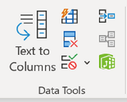
7. Finally, you can use the Remove Duplicates tool in Excel to quickly remove duplicate rows. On the Data tab, in the Data Tools group, click Remove Duplicates.

In the example below, Excel removes all identical rows (blue) except for the first identical row found (yellow).

Note: visit our page about removing duplicates to learn more about this great Excel tool.

The searching of duplicates in Excel – is one of the most common tasks for any of office employee. For its solution, there are a few different methods. But – how quickly to find duplicates in Excel and to highlight them with color? For the answer on this frequently asked question let us consider a concrete example.



How to find duplicate values in Excel?

For example we are engaging by check orders, which coming into the firm through Fax and e-mail. There can be such situation that the same order was by the two channels of incoming information. If you register twice the same order, there can be certain problems for the firm. Below we are considering to the decision by means of the conditional formatting.

For avoiding of the duplicate orders, you can use to the conditional formatting, which helps you quickly to find the duplicate values in Excel column.

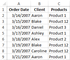
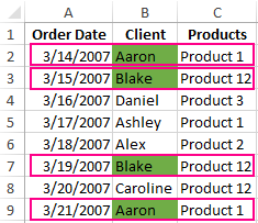
The example of the day orders for goods:

For verification whether the day orders are possible duplicates, we will analyze in the names of customers – there is the column B:

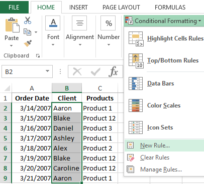
1. To highlight the range B2:B9 and then to select the instrument: «HOME» — «Styles» — «Conditional Formatting» — «New Rule».



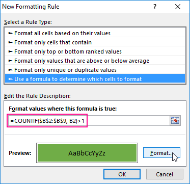
2. To choose «Use a formula to determine which cells to format».



3. To find the duplicate values in Excel column, you need to enter the formula in the input field:



4. After that you need to press the button «Format» and select to the desired cell shading to highlight duplicates in color — for example, green one. And click OK on all windows are opened.

Download an example of finding the Identifying Duplicate values in a column.

As can be seen in the picture with the conditional formatting we were able easily and quickly to implement the duplicate finder in function Excel and to detect to the duplicate data cells for the table of the day orders.



The example of COUNTIF function and highlighting of the duplicate values

The principle of the action formula for finding of the duplicates by the conditional formatting is simple. The formula contains the function =COUNTIF(). This function can also be used when searching for the identical values in the range of cells. The first argument in the function to the viewable data range is specified. In the second argument we specify what we are looking for. The first argument has an absolute reference, as it should be the same one. And the second argument conversely — should be changed on the address of the each cell in the viewing range, because it has a relative link one.

The fastest and the simplest ways: to find to the duplicates in the cells.

After the function we can see the comparison operator of the number of the found values in the range with the number 1. That is, if we see more, than one value means that the formula returns the value of TRUE and for the current cell is applied to the conditional formatting.

Duplicate values in Excel can be annoying, but fortunately, there are several methods for finding and removing them. We recommend making a backup copy of your Excel sheet before removing the duplicates. Let’s look at how to find, count, and remove duplicate values in Excel.

1. Use the Remove Duplicates Button

Excel comes with a native button to remove duplicate values.

1. Select the column where you would like to remove the duplicates.
2. Go to the “Data” tab and click the “Remove Duplicates” button.

1. The Duplicates warning box will appear, letting you customize your selection.
2. Select the “Continue with the current selection” option to remove duplicates from the currently selected data set.
3. To include more columns in the list, select “Expand the selection.”
4. Press the “Remove duplicates” button in both cases.

1. Keep the box checked next to the columns containing the duplicates and uncheck that you want to keep them.
2. Make sure the box next to “My data has headers” is selected. This will keep the first sets of data for duplicate values while removing their subsequent entries.

1. Click the OK button. Excel will remove all duplicate values and provide a summary of how many duplicate and unique values were found.

2. Find Duplicate Data Using Conditional Formatting

This method of removing duplicates is based on conditional formatting and will help you find duplicate values without deleting them.

1. In your Excel sheet, select the data that contains duplicates. It can be a column or the entire table.
2. Go to the “Home” tab and click on “Conditional Formatting.” The duplicate values will be highlighted.

1. Choose “Highlight Cell Rules” followed by “Duplicate Values.”

1. The “Duplicate Values” pop-up will appear, allowing you to change the color of duplicate values.
2. Click on the ‘Duplicate” drop-down box and select “Unique” if you want to see unique values instead.
3. Click on “OK.”

3. Remove Duplicates Using Conditional Filter

With the duplicates highlighted, you can either use filters to remove them or use the method shown above.

1. To activate the Filter operation, go to “Home tab → Sort & Filter → Filter.”

1. A drop-down box will appear next to the column headers in your data. Click on the drop-down box on the column where you would like to filter duplicates.
2. Select “Filter by color” from the menu. Choose the color of unique values to keep them in your sheet and remove the duplicates.

Now your sheet will only show unique values. Be careful as this method removes all the duplicate values including the first one.

To copy the unique values, select the data set and use the Alt + ; keyboard shortcut to select only the visible rows, then use the Ctrl + C shortcut to copy the visible rows and paste them wherever required.

4. Find Duplicate Values Using a Formula

Duplicates in a column can also be found using Excel formulas. The most basic formula for detecting duplicate entries is =COUNTIF(Range, Criteria) >1, where the range can be the entire column or a subset of rows.

Create a new column and enter one of the below commands in the new column.

• Use the formula =COUNTIF(D:D, D2) >1 for a full column, where D is the column name and D2 is the topmost cell.
• For selected rows, use the formula =COUNTIF($D$2:$D$10, $D2) >1, where the first set represents the selected rows, and D2 is the topmost cell. Please note that the range must be preceded by the dollar ($) sign, otherwise the cell reference will change when you drag the formula.

Drag the fill handle to use the command in the other rows. The formula will show “True” for duplicate values and “False” for unique values.

If you want to display some other text than True or False, you must enclose the COUNTIF formula in the IF function. So the formula will become =IF(COUNTIF($D$2:$D$10, $D2) > 1, "Duplicate”, “Single”).

If you want unique values to show a blank cell, use the formula =IF(COUNTIF($D$2:$D$10, $D2) > 1, “Duplicate”, “”).

5. Count Number of Duplicates Using a Formula

You can use the above formula without the > 1 text to count the number of duplicates in a column. The two formulas will become =COUNTIF($D$2:$D$10, $D2) and =COUNTIF(D:D, D2). Enter in the new column for it to display how many times each item appears in the data.

6. Remove Duplicate Values Using a Formula

Once you have found the duplicate values or the duplicate count, use the filter method to remove duplicates and retain unique values.

1. Go to “Home tab -> Sort & Filter -> Filter” to enable the filter drop-down box on the column header.
2. Click it and keep the box checked next to the value you want to keep. It should be “Unique” for the finding duplicates method and “1” for Counting duplicates. Doing so will hide the duplicate values and display unique values.
3. Select the visible rows using the Alt + ; shortcut.

7. Remove Duplicate Data Using Advanced Filters

1. Go to the “Data” tab and click on “Advanced.”

1. The “Advanced Filter” pop-up window will open.
2. Select the “Filter the list, in-place” option if you want to hide the duplicates on the same data set. You can manually copy-paste the unique values later to a different place in the same sheet or to a different sheet.
3. With this option selected, select the list of columns. They will automatically show up in the “List range” field. Leave “Criteria range” blank.
4. Check the box next to “Unique records only” and hit “OK.”

1. That will show unique values in your data. Use the Alt + ; shortcut to select visible rows only if you want to perform any action on them.
2. On the contrary, select “Copy to another location” if you want Excel to automatically copy the unique values to a different place in the same sheet.
3. Select the “List range” first. You can keep the “Criteria range” blank.
4. Click once on the “Copy to” field and select the rows on your sheet where you want to copy the unique data.
5. Make sure the box next to “Unique records only” is checked.

8. Remove Excel Duplicates Using Power Query

Power Query also helps to remove duplicate values in Excel as shown below.

1. Select the values where you want to remove duplicates.
2. Go to the “Data” tab and click on “From Table/Range.”

1. The “Power Query” editor will open. Select the columns and right-click on the selected column header. Choose “Remove duplicates” from the menu.

1. If you want to remove duplicates from the entire table, click on the “Table” button at the top-left corner and choose “Remove Duplicates.” Alternatively, select “Keep duplicates” to show only the duplicate entries and remove the rest.

1. Click on “Close and Load” at the top to open the table in the same sheet.

9. Using Pivot Tables

You can use Pivot tables to display only the unique values in your data, thus removing the duplicate entries.

1. Start by creating a Pivot table by selecting a cell inside your data.
2. Go to “Insert → Pivot table.” Select “From Table/Range.”

1. The PivotTable from the table or range pop-up will open.
2. Select the table or range where you want to hide duplicate values, for it to automatically show up in the “Table/Range” field.
3. Select whether the PivotTable should be placed in the same worksheet or in a new worksheet.
4. Click “OK.”

1. You will be greeted by the “PivotTable Fields” sidebar. Drag the columns where you to extract unique values to the “Rows” section.

You will need to format the PivotTable to show it in a tabular form. For that, go to the Data tab and perform the following steps:

1. Click on “Report Layout → Show” in tabular form.
2. Go to “Subtotals → Do not show subtotals.”
3. Click on “Report Layout → Repeat all item labels.”
4. Under “Grand Totals,” select “Off” for rows and columns.

You will get a Pivot table with unique values in a tabular form.

Read on to learn how to merge cells, columns, and rows to create a new set of data. And in case your worksheet contains important data, find out how to password protect your Excel workbook.