Due dates in excel

• 
  
  
  
  Excel Howtos, Learn Excel
  

Highlight due dates in Excel – Show items due, overdue and completed in different colors

• 
  Last updated on May 18, 2020

54 Responses to “Highlight due dates in Excel – Show items due, overdue and completed in different colors”

1. Peter says:

   Nice!
   Been using something like this for quite a while. Most companies use deadlines so this would be usefulle for everyone.

   • Gordon Bennett says:

     This is exactly what I need! However, I simply cannot get it to work! I’m using Excel 2010 and am completely replicating what you are doing, but it simply will not do it. Any advice from anyone would be greatly appreciated. PS EnableFormatConditions is set to True

     • S says:

       I had the same issue, but I think it was a formatting issue.

       Copy the formula from this website but delete the «» quotation marks. Type them back in from your own keyboard within the Conditional Formatting dialog boxes.

       Hope this helps.

2. Love it — although I often turn my books late anyway 🙁

3. Excel Challenged says:

   I am still not sure how the MEDIAN function works. When I print the value, it prints a random 5 digit number, But, when used in the formula, it does equate to the date which is weird. Why does it behave such ?
   =MEDIAN(TODAY()+1, $C6,TODAY()+7) in a cell returns a 5 digit # while
   =AND(MEDIAN(TODAY()+1,$C6,TODAY()+7)=$C6,$D6<>”Yes”) this seems to work just fine in Conditional formatting.

   • Shalabh Jain says:

     The 5 digit number that you see is the number of days elapsed since 1st Jan 1900 to the date in question. Excel uses this as a basis for all numeric operations on dates.

   • Following what Excel Challenged mentioned above,

     Change the Number format of the cell to DD MMM YY or whatever format you want.

4. Robert Clark says:

   Very clever use of Median — wouldn’t have thought of using it!

   @Excel Challenged:
   «The MEDIAN function, one of Excel’s statistical functions, shows you the middle number in a data list.
   Middle, in this case, refers to arithmetic value rather than the location of the numbers in a list.
   If there is an even set of numbers, the median is the average of the middle two values. «

   So, if we give three dates (start date, target date, end date), median will return the middle date of the three.  If target date is between the start and end dates, then the median function will return this.  If the target date is before the start date, then the median function will return the start date. If the target date is after the end date, then the median function will return the end date.

5. Jocelyn says:

   Can you change the dates to only fall on week days?  How?

   • @Jocelyn

     Can you please explain more about what you want to do?

     • Jocelyn says:

       We have an accounts payable spread sheet that has due dates of bills on it.  I would like the dates to only fall on weekdays since we do not work weekends.  Thank you for your help.

6. Sameer says:

   Ok, lets say if due date is 30 days plus date of invoice; then;

   =IF(AND(WEEKDAY(C13+30,2)>=1,WEEKDAY(C13+30,2)<=5),C13+30,IF(WEEKDAY(C13+30,2)=6,C13+32,C13+31))

   In the above; IF condition will check if weekday of due date is between 1 and 5 ie. 1 being monday and 5 being Friday.
   Then if this is true then it adds 30 days to the date of invoice, else it will add 31 days if due date is falling on sunday or add 32 days from date of invoice if its Saturday…

   Hope i got it right… Chandoo what do u think?

7. David says:

   How do I have the cell highlight just every 14 days after the date I manually enter in?

   I contact someone on the 1st and I want the cell to highlight on the 14th and that’s it. 

   • Jeremy says:

     To highlight 14 days and after the date you enter.
     =TODAY()<=a1+14
     Or
     To only highlight the 14th day after the date you enter.
     =TODAY()=a1+14

8. Jennie says:

   brilliant — this is just what I need,
   I wil be adding tasks to the spreadsheet so how can I copy the conditional formatting to other cells in the relevant columns please?

    
   Thank you

9. djograd says:

   Hi Chandoo! Very nice! Can this be done also in Google Spreadsheet? If not can you please show us a workaround or similar. Thank you. 

10. LARRY says:

    i have a formula i need to work out. im more of a novice and enjoy working with excel, however some of the more intense formulas escape me. i have followed this thread quite a bit and believe that i can use this to solve my problem, however i cant seem to grasp the specific verbage of the formula i need. i have 2 colums, one for PT test complet, one for PT test due, i have used a simple format of (=column1+180) to get my due date, what i need is to get the due date to highlight color 1-150 days after green, 151to 180 yellow and 181 days after red. help???

    • Hi Larry… Thanks for your comments.

      The simplest way to do this is, add an extra column (lets call it completed).

      Write the formula =today()-column1

      Now, use this column value to color the cells accordingly.

11. LARRY says:

    im not quite grasping this, can you give me an example?

12. LARRY says:

    when i do this, it returns the date as 1900

13. Steve says:

    Good stuff! It worked well for me, however, I now wish to apply the same CF to 2 columns, instead of a cell selction. When I do this, all the blank cells in the columns turn red. Is there a formula for «if blank do not format» or similar?

    • Steve says:

      No problem, I’ve worked it out…modified the last formula to read….
      =AND($D1>0,$D1<=TODAY()+28,$E1<>»YES»)
      The $D1>0 statement means that any blank cells are not formatted.

14. I’m wanting to figure out how i would do this for my job…i need to have orders signed by doctors and i’m wanting it to let me know when two weeks has passed and the order has not been received.

15. Yris says:

    Hello,

    I need help…..

    I am trying to make an employee spread sheet that will tell me when training is expired or about to expired or completed. I have an idea but I am still having trouble with the formula, I can do it in one cell but not for an entire column. It is not that big, one column for the employee names, next columns for the dates of the trainings. if training are completed I want them to turn green, if training are 30 days before expiration i want them to turn yellow and if they are expire i want them to turn red. any help please…
    thank you

16. Andries says:

    Please help if you can!
    I need to make a daily list of jobs with their due dates and then have three different things happening.
    1. When a job is completed/ticked off, it must removed from the list automaticaly
    2. From one day, before the due date, to 12:00am on the due date the cell colour of the whole row must be orange.
    3. After 12:00am on the due date the cell colour of the whole row must be red and stay red untill its ticked off as completed.

    I’ll really appreciate help in this, I’ve tried several formulas but I just don’t get it quite right.

    Regards

17. Mehaboob says:

    Hi sir
    it is very use full ,I have a doubt after making the due date ex:- in one sheet i have many customer each one have diffrent due due date and I make 12 sheet with month name is it possible to send the due date next sheet by month name , ex ; in JANUARY D1 due date is 12/9/13 I want send this to SEPTEMBER D1,and JAN D2 14/3/13 it need to go to march like this for every month

    I hope you can help me in matter I am really sorry my English is not good
    thanks Mehaboob

18. I have input all the formulas as the tutorial says but if there is no date put into the field it turns everything red. In other words I am trying to make a template at work with due dates and the orange part works great but everything is red unless I put a date into the cell. Any help would be awesome.

19. Jeff G says:

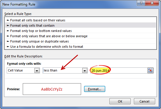
    If I want to use condtional formatting to indicate a red if the date entered is after June 20, 2014 and a green if it was completed prior to this date, how would I do this with condtional formatting?

    Thank you

    Jeff

    • Select the cell(s) where you would enter the dates. then,

      1. Go to conditional formatting > new rule
      2. Select the rule type as «Format cells that contain»
      3. Type the condition as below
      
      4. Set up formatting as needed.
      5. Repeat the rules for other date conditions.
      6. You are done

      • faisal says:

        DEAR SIR,

        PL:Date DUE DATE DAYS OVER Payment Received date

        I WANT THIS IF I ENTERED DATE IN PAYMENT RECEIVED DATE COL THEN DAYS OVER BECOME RECEIVED INSTEAD OF DAYS AND COLOR CHANGED AFTER ENTERED. CAN U GUIDE ME HOW ITS POSSIBLE

20. Jeff G says:

    Thank you

    So if I wanted it to show red if after the due date I would just set up that condition?

21. Jessie says:

    I have a column of when a person last took a class and a formula that created the date for when they must take it again, which is in three years. Works great. Now I want to color code the current year. For example: I took a class on 9/25/2012 and am due to retake it on 9/25/2015. I want that cell to turn red indicating that sometime during that year, I have to retake that class. I would even prefer to have the date change to JUST the year (so just «2015» instead of «9/25/2015»). Can you help me do this, please?

22. Wendy says:

    I really appreciate this post, but I’m confused about the MEDIAN. I assume that’s what selected the whole line of records rather than just what was in the 2 referenced columns. Why is that so?

23. james says:

    This might appear to be a silly question, but with the date highlighted when it becomes due/past can you get the cell to flash/blink on and off.
    I have just been asked this question i am using the latest excel

    Thank you in advance

24. Ravi says:

    I want that Once Due date is highlited with Red color , then it should remain highlighted with Red color on next day or untill i change the colour.

    Due date is highlited with color but next day it becomes without highlighting. I want it should remain highlited untill i change.

25. Juile says:

    Hi there,

    I really need help with this formula. Instead of a YES in the next column indicating that the task is complete, I need to enter a date to track our performance. Once a date is in the Completed Column, the date I am tracking would then turn Grey. I understand the due in 7 days and Past Due Formulas.

    I hope you can help! Thank you!

    • @Juile

      I’d recommend asking the question in the Chandoo.org Forums
      http://forum.chandoo.org/
      attach a sample file to speed up the response

26. sumeyyah says:

    please i need help, i want to do a conditional formatting: if 15 days left for the due date to color the cell red, if there is 2 months left for the due date to color the cell yellow, if more than 2 months left for the due date i want the color of the cell to be green.

    please i need the formula for that, ive been struggling all day.

    • Brenda says:

      My issue is similar to this. I have one due date for number of tasks and would like to add conditional formatted depending on whether a task is completed or how many days there are until the due date.
      -if no date is entered withing 2 days of the due date — highlight yellow
      -if no date is entered by the due date — highlight red
      -if a date is entered by the the due date — highlight green

      I have tried a number of formulas and conditional formatting scenarios but have had no luck. Thanks in advance.

27. Dwarkanath bari says:

    i want to generate dates if design actual date is delay for 2 days then for costing department date is increase by delay date.

    design target actual complete costing target marketing target

    05-04-2016 07-04-2016 09-04-2016 10-04-2016

    in above design target date is 05/04/2016 but design task completed on 07-04-2016 so costing target date will be automatically calculated as per delay days.

28. Russell says:

    =AND(MEDIAN(TODAY()+1,$C6,TODAY()+7)=$C6,$D6”Yes”)

    This is only for 7 days.
    What if I want it to be exactly 2 months away? Or even 1 year away? Any guidance on this? Sorry im very new to excel.

29. Heidi says:

    I tried to do a variation on this, we are setting up reminders to follow up on emails.

    Column N has date last followed up

    Column O is labeled ‘Application Recieved’ (If I has been received we type YES, if not it is blank)

    First line of data is row 9.

    I am in the process of creating 3 rules to change the cell/words according on where we are up to:

    1. The application form has been received (YES is in ‘O9’), therefore ‘N9’ and ‘O9’ cells turn white and text grey.

    =$O9=»Yes»

    This is working.

    2. If the date in ‘N9’ is less than 7 days old = Yellow cell.

    =AND(TODAY()-$N9>=7,$O9”Yes”)

    Not working. 🙁

    3. If the date in ‘N9’ is more than 7 days old = Orange cell.

    =AND($N9<=TODAY()+7,$O9”Yes”)

    Not working. 🙁

    Love any help you can offer…

30. Heidi says:

    We are setting up reminders to follow up on emails.

    Column N has date last followed up

    Column O is labled ‘Application Form’ (If I has been received we type YES, if not it is blank)

    First line of data is row 9.

    I am in the process of creating 3 rules to change the cell/words according on where we are up to:

    1. The application form has been received (YES is in ‘O9’), therefore ‘N9’ and ‘O9’ cells turn white and text grey.

    =$O9=»Yes»

    This is working.

    2. If the date in ‘N9’ is less than 7 days old = Yellow cell.

    =AND(TODAY()-$N9>=7,$O9”Yes”)

    Not working. 🙁

    3. If the date in ‘N9’ is more than 7 days old = Orange cell.

    =AND($N9<=TODAY()+7,$O9”Yes”)

    Not working. 🙁

    Love any help you can offer…

    Reply

31. Ahmad says:

    Hi, I’ve solved this without median and AND functions.

    You’ve used median and AND function in everywhere to avoid «yes». We can avoid «yes» issue by lifting «yes» rule to the top of conditional format rules from manage rules, right? in this case «yes» will be on top of other rules and we don’t need to write «yes» in each next rule.

    ‘m just wondering why you didn’t used like this and preferred median+AND function? is there some moments that I’m missing?

    Please clarify for me 🙂

32. Bobbie says:

    what is the formula for using a red flag. I would like to apply this concept to a task/project list and would like a red flag to appear in one cell when a task/project is overdue.
    thank you!

33. James says:

    Hi,

    I am tracking the dates of wage assessments for various positions throughout my organization. We like to preform a market wage assessment every 3 years for every position in our organization. I used the formulas you suggested (minus the column D part with a Yes or No question because not applicable for us. I set up the formulas to show red with positions that are past the 3 year mark and set the other two up to show me ones that are due within 3 months or 6 months. However even ones that are due 3 years from now (newly completed wage assessment), excel is still highlighting these positions red like they are past due. Please advise how I can get the cells of positions that are not past due to stay white/ no fill.

    Thanks,

    James

    • Can you share the condition that you used? It is possible that your condition is returning false positives.

      • James says:

        Sure. I am trying to highlight dates for future and past due wage analysis. These are the conditions I have entered:

        Red: =AND($E$2=TODAY())

        For Red I want to show Assessments that are past due (for us that means no wage assessment has been completed in the past 3 calendar years)
        For Yellow I want to show Assessments that are due within the next 3 months
        For Green I want to show Assessments that are due this year.
        For White/ No Fill I want to show Assessments that are no due at this time ( meaning they have a completed assessment sometime in the past two years.

        I put the date of the last assessment in Column D and then add 1096 days to the date for each position to show when he next assessment is due in column E ( so all of Column E are formula values )

        Please let me know if you have any questions or if I need to provide more detail.

        Thank you,
        James

        • James says:

          Sorry, the rest of my conditions did not show in my reply. I have listed them below:
          Red: =AND($E$2=TODAY())

          • James says:

            Yellow: =AND(MEDIAN(TODAY()+1,$E2,TODAY()+91.3333)=$E2)

          • James says:

            Green: =AND(MEDIAN(TODAY()+91.34,$E2,TODAY()+364.5)=$E2)

          • James says:

            White/ No Fill: =AND($E$2>=TODAY())

34. James says:

    Yellow: =AND(MEDIAN(TODAY()+1,$E2,TODAY()+91.3333)=$E2)

35. Brian says:

    Great article.

    How would I go about having cells highlighted by time lapsed for things that are repeated every few months? Say I have a cell that contains a date of March 13th, and I want it to be green for 3 months, then orange for 3 months, then red after 6 months?

Leave a Reply

We welcome your comments and questions about this lesson. We don’t welcome spam. Our readers get a lot of value out of the comments and answers on our lessons and spam hurts that experience. Our spam filter is pretty good at stopping bots from posting spam, and our admins are quick to delete spam that does get through. We know that bots don’t read messages like this, but there are people out there who manually post spam. I repeat — we delete all spam, and if we see repeated posts from a given IP address, we’ll block the IP address. So don’t waste your time, or ours. One other point to note — if you post a link in your comment, it will automatically be deleted.

Add a comment to this lesson