Drop down list excel dependent

This example describes how to create dependent drop-down lists in Excel. Here’s what we are trying to achieve:

The user selects Pizza from a drop-down list.

As a result, a second drop-down list contains the Pizza items.

To create these dependent drop-down lists, execute the following steps.

1. On the second sheet, create the following named ranges.

Name	Range Address
Food	A1:A3
Pizza	B1:B4
Pancakes	C1:C2
Chinese	D1:D3

2. On the first sheet, select cell B1.

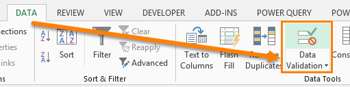
3. On the Data tab, in the Data Tools group, click Data Validation.

The ‘Data Validation’ dialog box appears.

4. In the Allow box, click List.

5. Click in the Source box and type =Food.

6. Click OK.

Result:

7. Next, select cell E1.

8. In the Allow box, click List.

9. Click in the Source box and type =INDIRECT($B$1).

10. Click OK.

Result:

Explanation: the INDIRECT function returns the reference specified by a text string. For example, the user selects Chinese from the first drop-down list. =INDIRECT($B$1) returns the Chinese reference. As a result, the second drop-down lists contains the Chinese items.

Home / Advanced Excel / How to Create a Dependent Drop-Down List in Excel

The dependent drop-down is all about showing values in a drop-down list according to the selection of the value in another drop-down.

Today, in this post, I’d like to share with you a Simple 7-Steps Process to create this drop-down. But first of all, let me tell you why it is important. In the below example, you have two drop-down lists. The size drop-down is dependent on the product drop-down.

If you select the white paper in the product cell then in size drop-down will show small and medium. But, if you select gray paper then its size will be medium and large.

So here the basic idea to create a dependent drop-down list is to get the correct size as per the product name. Let’s get started.

For creating a dependent drop-down list we need to use named ranges and indirect functions.

• First of all, you have to create named ranges for drop-down lists. For this, select the product list. Go to -> Formulas -> Defined Names -> Create from selection.

• You’ll get a pop-up. Tick mark “Top Row” & click OK.

• By using the same steps, create two more named ranges for sizes. One is for white paper and the second is for the gray paper.

Quick Tip: By using this method to create a named range, the value in the first cell will be considered as the name, and the rest of the values as the range. You can also use a dynamic named range for this.

• Now select the cell where you want to add the product drop-down and Go to -> Data -> Data Tools -> Data Validation.

• In the data validation window, select “List” and in “Source” enter the below formula and then click OK.

=Indirect(“Product”)

• Select the cell where you want to add a size drop-down list. Go to -> Data -> Data Tools -> Data Validation.
• In the data validation window, select “List” and in “Source” enter the below formula and click OK.

=Indirect(“A5”)

Finally, your dependent drop-down list is ready.

How Does it Work

First, you have created three named ranges. Then we used one named range to create a product drop-down. After that, for the second drop-down list, you have used the indirect function & refer to the value in the product cell.

If you notice, our size-named ranges have a name equal to the values we have in the product drop-down.

When we select “WhitePaperSheet” in the product cell, then in the size cell indirect function refers to the named range “WhitePaperSheet” and when you select “GreyPaperSheet” it will refer to the named range “GreyPaperSheet”.

Three-Level Dependent Drop-Down List

In the above example, you have created a two-level dependent drop-down list. But sometimes, we need to create a list with three-level dependencies. For this, all you have to do is create a third drop-down list which is dependent on the selection of the second drop-down list.

Let’s say we want to add a drop-down list with “Length x Width” of the sizes for paper sheets.

And, for this, you have to create a third drop-down list that will show the “Length X Width” as per size selection.

Here are the steps:

• Create three more named ranges using the same method which we have used above.

• Select the cell where you want to insert your third drop-down.
• Open drop-down options & insert the following formula in the source.

=Indirect(“C5”)

• Click OK.

Now, your three-level drop-down list is ready

sample-file

We begin with a table of Divisions where each Division contains a list of Apps.

The goal is to have the user select from the first drop down list a Division name.  Next, the user will select an App from the second drop down list.  The key is to only display the apps associated with the selected Division from the first drop down list.

NOTE: In the real world, the list of Divisions and Apps would likely be placed on a separate (possible hidden) sheet, or the list would be placed somewhere far away from the data entry portion of the sheet where the user is not likely to ever find.  For this example, we are placing the list close to the user-area to make the demonstration easier to follow.

Creating the First Drop Down List (Division)

The first drop down list will allow the user to select a Division.  This one is simple.

We begin by creating a Data Validation drop down list for cell A5 that points to the Divisions listed in cells F4 through H4.

1. Select cell A5
2. Select Data (tab) -> Data Tools (group) -> Data Validation
3. In the Data Validation dialog box, set Allow to “List” and Source to “=$F$4:$H$4”
4. Click OK

To get the drop down list to appear for multiple rows, select A5 and copy/paste the contents to adjacent cells (ex: A6:A20).

Creating the Second Drop Down List (App)

As stated earlier, we want the second list of Apps to only show items based on the selected Division from the first drop down list.

Using the OFFSET function

We will use the OFFSET function to select Apps from one of the three listed Divisions.

If you’re not familiar with the OFFSET function, it allows us to start from a defined point then moves away from that point by a set number of rows and/or columns.  This establishes a new start point.  From here, we can select a set number of rows and/or columns.

The OFFSET function has the following syntax:

OFFSET(reference, rows, cols, [height], [width])

• reference – the cell or range of cells you want to base the offset (e. the starting point).
• rows – the number of rows down or up you want to move. A positive number moves down; a negative number moves up.
• cols – the number of columns right or left you want to move. A positive number moves right; a negative number moves left.
• [height] – the number of rows you want returned. This must be a positive number.
• [width] – the number of columns you want returned. This must be a positive number.

NOTE: For an explanation of the OFFSET function, see this post/video.

Ultimately, we need to create this formula in the Data Validation dialog box.

Since the Data Validation dialog box does not possess the IntelliSense feature that is so helpful when writing formulas, we will write and test our formula in a standard Excel cell.

Once we have the formula working, we will transfer it to the Data Validation tool for its final test.

Establishing the Starting Point

We will always begin our search for Apps from the upper-left corner of our table (cell F4).

Start the OFFSET function as follows.

=OFFSET($F$4

We need to make this reference to cell A4 as an absolute reference so each copied/pasted version begins from the same point.

Moving Down or Up

Next, we tell OFFSET how many rows to move down or up.  The Apps list begins 1 row below our start point, so we assign a value of 1 to the rows argument.

=OFFSET($F$4, 1

Moving Right or Left

Now we tell OFFSET how many columns to move right or left.

This is determined by the user’s Division selection from the first drop down list.

For this, we can use the MATCH function to locate the selected Division in cell A5 from the list of Division in cells F4 through H4.  We also need to match exactly (0 in the last argument).

=OFFSET($F$4, 1, MATCH($A5, $F$4:$H$4, 0)

NOTE: We only “locked” the “A” part of the “A5” reference because we don’t want to point to other columns when we replicate this to adjacent cells, but we do want to point to other rows when creating additional drop downs.  If that’s a bit unclear, stick with us because it will become clearer very soon.

If we highlight the MATCH portion of the formula and press F9, we can see MATCH returns a number indicating the discovered position in the search range.

NOTE: Remember to press CTRL-Z to undo your formula back to its original structure.

The Problem with MATCH

A minor issue we have with MATCH is that it counts cells beginning with the value 1.

This means that “Productivity” is in the first column of the data, “Game” is in the second column, and “Utility” is in the third column.

Because we’re trying to inform OFFSET how many columns to move to the right, these values are incorrect.

If we want “Productivity”, we don’t want to move left or right.  If we want “Game”, we want to move 1 column to the right, and if we want “Utility”, we want to move 2 columns to the right.

We need to reduce the returned value of MATCH by 1 to adjust for this discrepancy.

=OFFSET($F$4, 1, MATCH($A5, $F$4:$H$4, 0) – 1

Selecting the Height to Return

We dropped 1 row from the start point to land on the first App.  We also moved right to the proper Division column.

The tricky part is to determine the number of rows to select.  This will be the list of Apps that will drives the second drop down list.

Notice that our three lists do not contain the same number of items.

Temporarily, we will treat each list as if they contained 15 items.  This will allow us to see if the [height] argument is working.  Later, we’ll make the height selection dynamic so it will return the perfect number of Apps for our second drop down list.

=OFFSET($F$4, 1, MATCH($A5, $F$4:$H$4, 0) – 1, 15

For any columns that contain less than 15 Apps, this will produce empty slots in the Data Validation drop down list.  If you’re okay with that, you can leave the [height] argument set to the largest expected list length.  This could be a problem if one list has hundreds of items while another list has only dozens.

Like I said a moment ago, we’ll start statically then make it dynamic later, so we eliminate the empty slots.

Selecting the Width to Return

We only ever want a single column of Apps to be returned by the OFFSET function, so we will set the [width] argument to 1.

=OFFSET($F$4, 1, MATCH($A5, $F$4:$H$4, 0) – 1, 15, 1)

Setting Up Data Validation

Now that we have completed our test formula, it’s time to use the logic in a Data Validation drop down list.

1. Select cell B5
2. Highlight the OFFSET/MATCH formula displayed in the Formula Bar
3. Copy the formula to memory
4. Press ESC to get out of Edit Mode
5. Select Data (tab) -> Data Tools (group) -> Data Validation
6. In the Data Validation dialog box, set Allow to “List”
7. In the Source field, paste the recently copied OFFSET/MATCH formula
8. Click OK

Testing the OFFSET/MATCH Formula

If we select a Division from the first drop down list (A5), we then see the list of related Apps in the second drop down list (B5).

Because we are using a fixed [height] argument, we see blank slots for any Division where the Apps list is less than 15.

Getting the Perfect Height

To get a list of Apps that do not display blank slots at the bottom, we need to calculate the height of the selected Division’s Apps.

We need to take the previously hard-coded “15” for the [height] argument and make it dynamic.

Enter the COUNTA Function

A perfect way to determine the number of Apps in a give Division is to use the COUNTA function.

As a test, we select an unused cell in our sheet and write the following formula:

=COUNTA(F5:F19)

This yields a result of 15.

If we point the COUNTA function to G5:G19, we get 12, and if we point the COUNTA function to H5:H19, we get 13.

We don’t want to hard-code the count range, we want the range to be based on the selected Division.

We can replace the hard-coded range with the same OFFSET formula used earlier.

=COUNTA(OFFSET($F$4, 1, MATCH($A5, $F$4:$H$4, 0) – 1, 15, 1)

NOTE: the “15” defined in the [height] argument represents the largest number of Apps we would expect to see in any given Division.  You should set this value to whatever number you believe you would never reach, such as =COUNTA(OFFSET($F$4, 1, MATCH($A5, $F$4:$H$4, 0) – 1, 500, 1).

Testing the COUNTA Formula

In cell A5, if we select “Productivity” we are returned a value of 15.  If we select “Game” we are returned a value of 12, and if we select “Utility” we are returned a value of 13.

Updating the Data Validation Formula

Our final step is to update the formula previously placed in the Data Validation tool for cell B5 to include this dynamic logic for [height] calculations.

1. Select the cell that contains the temporary COUNTA formula
2. Highlight the COUNTA/OFFSET formula displayed in the Formula Bar
3. Copy the formula to memory
4. Press ESC to get out of Edit Mode
5. Select cell B5
6. Select Data (tab) -> Data Tools (group) -> Data Validation
7. In the Source field, remove the “15” from the original formula and paste the recently copied COUNTA/OFFSET formula
8. Click OK

=OFFSET($F$4, 1, MATCH($A5, $F$4:$H$4, 0) – 1, COUNTA(OFFSET($F$4, 1, MATCH($A5, $F$4:$H$4, 0) – 1, 15, 1)), 1)

Testing the Updated Formula

If we select a Division form cell A5 that has less than 15 Apps, we are no longer presented with empty slots at the bottom of the Apps drop down list (B5).

Copying the Data Validation to Adjacent Cells

To replicate the second Data Validation drop down list to the row cells below cell B5:

1. Select cell B5
2. Press Copy
3. Select your destination cells (ex: B6:B15)
4. Right-click the highlighted range and select “Paste Special…”
5. In the Paste Special dialog box, select Validation and click OK

Final Test

You are now able to select a cell from the “Select Division” column, select a Division, then click the corresponding “Select App” cell to be presented with the Apps for the selected Division.

Granted, I did say that we would use a single formula.  I never said it would be short and simple.

The nice thing is that with a small bit of practice, this formula is fairly easy to write.  You could even copy/paste it form project to project, reusing it with just minor modifications.

I think it’s easier to stick to a single strategy for building these dependent drop down lists and get good at it, versus learning dozens of other techniques.

Yes, some of those other techniques may be more efficient or have more features, but unless you need fancy and exotic, this one will do just fine.

Practice Workbook

Feel free to Download the Workbook HERE.

Bottom line: Learn how to create cascading or dependent drop-down lists (also known as cascading validation) in Excel.  This technique does NOT require named ranges.  If you don’t mind using named ranges then there are a few links at the bottom of the page with solutions that will be easier to implement.

Skill level: Intermediate

Functions used: OFFSET, MATCH, COUNTA, COUNTIF, INDIRECT

Drop-Down (Data Validation) Lists

Before we dive into dependent lists, if you are unfamiliar with drop-down lists in general (also known as data-validation lists), I strongly suggest you check out my tutorial for creating drop-down lists and also this post for making drop-down lists dynamic.

What is a Dependent Drop-down List?

Leah asked the following question, “How do I create a drop-down list where the list of choices changes when I select an item in another list?”

You can see an example of this in the screencast below.  When I select “Coffee” from the validation list in cell B4, the list in cell E4 displays different types of Coffee.

When I select “Wine” from the list in cell B4, the list in cell E4 displays different types of Wine.

These are called dependent or cascading drop-down lists because the 2nd list depends on the choice made in the first list.  This technique requires the use of the OFFSET function to create the dependencies, and it’s a great function to learn.

Step-by-Step Guide to Dependent Drop-down Lists

The rest of this article will explain how to create these dependent lists in your own workbook.  You can also download the example file to follow along, or just copy the sheets into your workbook.

Step 1: Prepare the Source Tables

Our first step is to create the source tables that we will use for the contents of the drop-down lists.

In the image above, the ‘Lists’ sheet contains the lists for each drop-down.  The list in column B contains the Category items for the parent list.  The parent list is the list where we will make the first choice.

We then use the list in columns D:F on the ‘Lists’ sheet to populate the child list with items.  The child list is the second list of choices that will be dependent on the selection in the parent list.

The first column in this table (column D) contains the Categories.  These are the exact same names that are in column B.  The second column in the table (column E) contains the different types for each category.  This is where the relationship between the Category and Type are created.

It’s also important to note that the child list needs to be sorted for this technique to work.  In the image below you can see that I sorted column D so that all the Category items are grouped together in the list.

These lists originated from a much larger data table that contains transactional sales data.  To create the lists I needed to extract all the unique values for each list.

Fortunately, Excel has some great built-in tools that allow you to remove the duplicates.

One way is to use the Remove Duplicates tool that is located on the Data tab in the ribbon.

You could also create a pivot table to quickly list the unique values in the Rows area of the pivot.  Then copy/paste the results to the ‘Lists’ sheet that contains the source tables.

I won’t go into details on these techniques, but they will make it very fast to create and update you dependent lists.  If your lists change frequently with new items, then I would recommend the pivot table method because you can simply refresh the pivot table to generate your new list.

Step 2: Create the Parent Drop-down List

Ok, now that we have the source data lists setup we can create the drop-down lists.  We will do this with in-cell data validation lists.

Dependent drop-down lists are not a built-in feature of Excel.  Therefore, we need to get creative with some functions and formulas to create the dynamic dependencies between the lists.

With cell B6 selected on the ‘Dropdowns’ sheet, click the Data Validation button on the Data tab of the ribbon.

The Data Validation window will appear.

1. First, choose “List” in the Allow drop-down list.
2. Then enter the OFFSET formula in the Source box (see explanation below).
3. Press OK.

We could put the following reference in as the Source: =Lists!B2:B4

However, we want the source list to be dynamic.  Dynamic means that the list will automatically expand as we add more items to it.  We don’t want to have to change the source reference every time we add items to the list.

The OFFSET function helps create this dynamic range reference, and returns a reference to a range of cells based on the coordinates you specify.  It has the following arguments.

=OFFSET(reference, rows, columns, [height], [width])

Our Formula: =OFFSET(Lists!B1,1,0,COUNTA(Lists!B:B)-1,1)

Here is a quick explanation of each argument in the formula:

• Reference – Think of this as the cell that is the starting point for the range.  In this case we are starting in cell B1 on the ‘Lists’ sheet.
• Rows – We actually want to move the starting point down to cell B2.  The rows argument allows us to specify how many rows down we should move (offset) the starting point. We put a “1” for this argument to move the starting point down to cell B2.
• Columns – This argument would move the starting point to the right a specific number of columns.  In this case we want to stay in column B, so we leave this argument blank or put 0 (zero).
• Height – This is the height of the range specified in number of rows.  In this case we are using the COUNTA function to count the number of rows that contain text in column B. =COUNTA(Lists!B:B).  This will return 4 since there are 4 rows with text in column B.  We subtract 1 because we don’t want to include the header row in our list.
• Width – This is the width of the range specified by number of columns.  Our range is only 1 column wide (column B) so we put a 1 here.

You should now have a drop-down list in cell B6 that contains all the Category items in the list on the Lists tab.

Excel Tables and the Structured Reference Alternative

If you are storing your lists in Excel Tables (which I highly recommend), then you could use the following formula instead.

=INDIRECT(“tblCategory[Category]”)

Since Table references expand and collapse automatically when rows are added/deleted, you do not need to use the OFFSET function.

Step 3: Create the Child (Dependent) Drop-down List

We now need to create the child list, which is dependent on the selection of the parent list.

The OFFSET function can be used for this list as well.  We just need to make a few adjustments to make it dependent on the selection in the parent list.

Here is the formula for the child list:

=OFFSET(Lists!$D$1,MATCH(B6,Lists!$D:$D,0)-1,1,COUNTIF(Lists!$D:$D,B6),1)

Here is an explanation of each argument in the OFFSET formula:

• Reference – Start in cell D1 on the Lists tab.  This is the top left cell of the table that lists the child items.
• Rows – Use the MATCH function to find the first row that matches the item selected in the parent list.  Cell B6 is the reference to the cell that contains the parent drop-down list.  This is basically a lookup function that returns the row number of the first matching item.  Subtract one to account for the header row.
• Columns – Specify a “1” to move one column to the right.  The formula is going to find the matching range in column D, then we have to move over one column to the right to return the range of matching values in column E.
• Height – Use the COUNTIF function to count the number of occurrences of the parent item in Cell B6, “Coffee”.  This returns a 4, which means the range will be 4 rows high.
• Width – The range is one column wide (column E).

The child drop-down list in cell E6 should now be dependent on the selection made in cell B6 on the ‘Dropdowns’ sheet (parent list).

Excel Tables and the Structured Reference Alternative

As an alternative, you could use the structured reference formulas with the Excel Table names instead of cell addresses.  The Table formula would look like the following.

=OFFSET(INDIRECT(“tblType[#Headers]”), MATCH(B11,INDIRECT(“tblType[Category]”),0), 1, COUNTIF(INDIRECT(“tblType[Category]”),B11),1)

It’s not as pretty because you have to add the INDIRECT function for each table reference.

Dependent Drop-downs WITHOUT Named Ranges

There are a few different ways to create dependent drop down lists in Excel.  The main advantage of this method is that it does NOT required the use of named ranges.

Named ranges are a great feature, but can be very confusing for some users.  Therefore, I recommend not using named ranges unless you are confident that all future users of your model will understand them.

If you don’t mind using named ranges then the following articles provide some awesome tutorials on other ways to create the drop-downs.

• Create Dependent Lists With INDEX by Roger Grovier at Contextures
• Dependent Drop Down Lists from a Sorted List by Debra Degleish at Contextrures
• Create Dependent Drop-down Lists with Conditional Data Validation  & Slicers as an Alternative to Conditional Drop Downs by Jeff Lenning at Excel University
• Great VBA & Non-VBA solutions by Jeff Weir and Roberto Mensa over at Chandoo.org

Download the Sample Workbook

You can download the sample workbook below to follow along, or simply copy the sheets into your own workbook.

How to Search a Drop-down List

Excel doesn’t have a built-in option to search drop-down lists for a particular item, but I’ve created an add-in that gives you that option.  It’s called List Search and you can access that add-in here:

Click here to download the List Search Add-in

I hope this post is useful for you! Please leave a comment below with any questions or suggestions.