

Data entry is quicker and more accurate when you use a drop-down list to limit the entries people can make in a cell. When someone selects a cell, the drop-down list’s down-arrow appears, and they can click it and make a selection.
Create a drop-down list
You can make a worksheet more efficient by providing drop-down lists. Someone using your worksheet clicks an arrow, and then clicks an entry in the list.
-
Select the cells that you want to contain the lists.
-
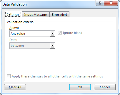
On the ribbon, click DATA > Data Validation.
-
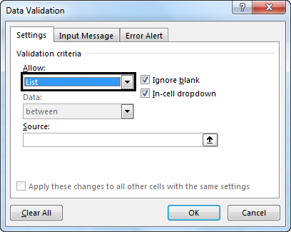
In the dialog, set Allow to List.
-
Click in Source, type the text or numbers (separated by commas, for a comma-delimited list) that you want in your drop-down list, and click OK.
Want more?
Create a drop-down list
Add or remove items from a drop-down list
Remove a drop-down list
Lock cells to protect them
Data entry is quicker and more accurate when you use a drop-down list to limit the entries that people can make in a cell.
When you select a cell, the drop-down list’s down-arrow appears, click it, and make a selection.
Here is how to create drop-down lists: Select the cells that you want to contain the lists.
On the ribbon, click the DATA tab, and click Data Validation.
In the dialog, set Allow to List.
Click in Source.
In this example, we are using a comma-delimited list.
The text or numbers we type in the Source field are separated by commas.
And click OK. The cells now have a drop-down list.
Up next, Drop-down list settings.
Need more help?
Want more options?
Explore subscription benefits, browse training courses, learn how to secure your device, and more.
Communities help you ask and answer questions, give feedback, and hear from experts with rich knowledge.
Before we edit drop-down lists in Excel, we must know what a list in Excel is. In simplified terms, lists in Excel are columns in Excel. But in columns, we do not have any drop-downs. Instead, we enter values manually or paste the data from any other source. But, if we are creating surveys or asking any other user to enter data and want to give some specific options to choose from, drop-downs in Excel come in handy.
As explained above, drop-downs in Excel help guide a user to manually enter values in a cell with some specific values to choose from. Like in surveys, if there is a question about the gender of a person, if we ask every user to enter values for that question, then data will not be in order. Some people may write answers in uppercase, some in lowercase, or some may make some spelling mistakes. But if we give users two values to choose from, either male or female, our data would be in the exact order we want. It is done by creating a drop-down lists in excelA drop-down list in excel is a pre-defined list of inputs that allows users to select an option.read more.
There are various ways of editing drop-down lists in Excel. They are:
- Giving drop-down values manually and using data validation.
- Offering drop-down ranges and using data validation.
- Creating a table and using data validation.
The data validation is an option under the “Data” tab in the “Data Tools” section.
Table of contents
- Editing Drop-Down List in Excel
- How to Edit Drop-Down List in Excel?
- Example #1 – Giving Drop Down Values Manually and Using Data Validation.
- Example #2 – Giving Drop Down Ranges and Using Data Validation.
- Example #3 – Creating a Data Table and Using Data Validation.
- Explanation of Edit Drop-Down List in Excel
- Things to Remember While Editing Drop-Down List in Excel
- Recommended Articles
- How to Edit Drop-Down List in Excel?
How to Edit Drop-Down List in Excel?
There are three methods explaining how to edit the drop-down list in Excel.
Let us learn to make drop-down lists with some examples and learn every process to edit the drop-down list in Excel.
You can download this Edit Drop-Down List Excel Template here – Edit Drop-Down List Excel Template
Example #1 – Giving Drop Down Values Manually and Using Data Validation.
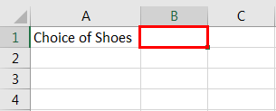
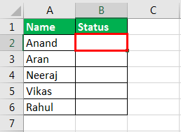
We need to have the drop-down values ready to enter for the step. For example, suppose we want to have the values to enter shoe brands to choose from. Now, we need to select a cell where we will insert the drop-down.
- In cell B2, we will enter our drop-down list.

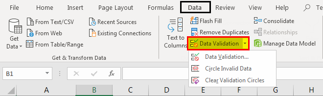
- Next, click on “Data Validation” in the “Data” tab under the “Data Tools” section.

- Again, click on “Data Validation” in Excel, and a dialog box appears.

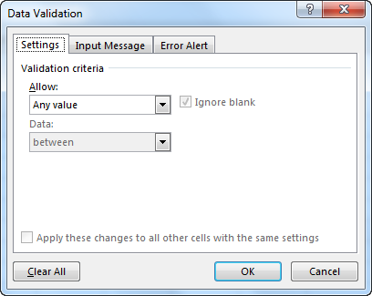
- In “Settings,” under the “Allow,” select “List.”
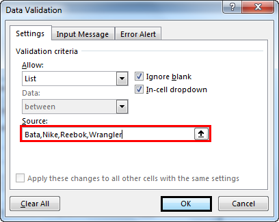
- In the “Source” section, we must manually enter the values for the drop-down options.
- When we click on the “OK,” we may have our drop-down created.

The above method is the easiest way to make and edit a drop-down list in Excel. But, if we have to enter more values for the choice of shoes, we have to redo the whole process.

Example #2 – Giving Drop Down Ranges and Using Data Validation.
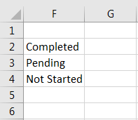
For example, I am a teacher, and I want a response from my students whether they have completed their projects or not. Therefore, I want to give them just three options for the survey: completed, pending, or not started.
Yes, I can use the above process, but the user can change it as they can go to the “Data Validation” tab and change the values. In this process, we select a range of values and hide the columns so that the other user cannot edit the validation or the dropdown.
- We must copy values for drop-downs or write them down in a list or column.
- In the cell we want to enter the validation, we will select the cell, cell B2.
- Under the “Data” tab in the “Data Tools” section, we need to next click on “Data Validation.”

- Again, we need to click on “Data Validation.” As a result, a wizard box appears.
- In the settings, under “Allow,” click on “List.”
- In the “Source” tab, we must select the range of data for the drop-down list.
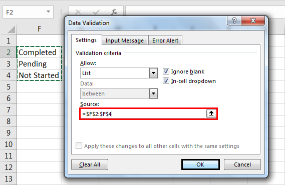
- When we click on “OK,” we may have a drop-down in cell B2.
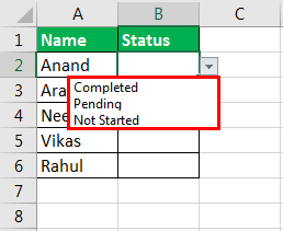
- After that, we need to copy the validation to all the cells (up to cell B6). Then, finally, we have to drop down a list of all the cells we want.

Even if we hide our cell range, which was the drop-down source, any user cannot edit the validation. The above process also has the same disadvantage as the first example. If we have to insert another option of “Half Completed,” we have to redo the process again. I have to insert a new alternative to the source and new validation.
Example #3 – Creating a Data Table and Using Data Validation.
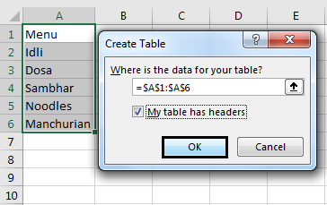
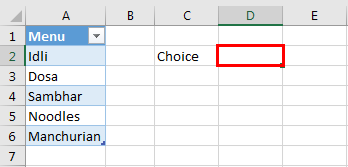
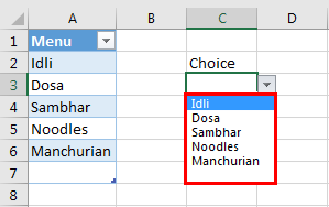
We will create a data table and use data validation as before in this method. But it will explain the benefit of using this method later on. For example, I have a restaurant and have some dishes to select for customers. So I have inserted the data in the column below.

- The first step is to create a table. Then, we must select the data, and in the “Insert” tab, click on “Tables.”

- The following window will open, and when we click “OK,” we have created our table in column A.

- Let us name this table “Restaurant.” In the left corner, we can see an option to rename the table.
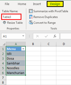
- Rename the table as “Restaurant.”

- Now, we must select the cell where we want to insert the drop-down list.
- Under the “Data” tab, now we must click on “Data Validation.”
- In the “Allow” tab, select “List.”
- Now in “Source,” type as shown in the dialog box below.

- When we click on “OK,” we can see that a drop-down has been inserted into the data.
- If we have another menu to add, suppose “Soups.”

- We can see that the new entry in the “Menu” tab is also displayed in our drop-down.
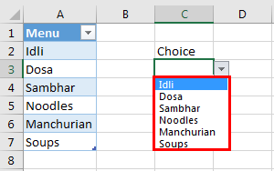
The above process has solved our problem: a new entry has to be created, and we must make drop-downs again.
Explanation of Edit Drop-Down List in Excel
I have already explained above why we need drop-down lists in our data. It helps guide a user to manually enter values in a cell with specific values to choose from.
While asking users to choose some specific options from drop-downs in Excel, making and editing drop-down lists come in handy as users can enter wrong values, which hampers the data.
Things to Remember While Editing Drop-Down List in Excel
- If we enter drop-down values manually or set ranges, any newer entry needs to be inserted with a new drop-down list.
- In tables, we can insert a new entry, updated in the dropdown.
- To view or edit the drop-down list, we need to click on the cell.
Recommended Articles
This article is a guide to Edit Drop-Down List in Excel. Here, we discuss editing a drop-down list in Excel and examples and downloadable Excel templates. You may also look at these useful functions in Excel: –
- Search For Text in Excel
- Excel Column Number
- Excel Columns Group
- Randomize List Excel
In this article, we will learn how to edit the dropdown option on cells.
Data Validation is an Excel 2016 feature whose purpose is to restrict what users can input into a cell. It is essential to create drop-down lists or combo boxes that contain predefined options that limit user errors and allow for more consistent data entry.
In this article, we are going to learn how to edit dropdown list in excel. To do this, we will use the Name manager and Data Validation.
Let’s understand this by taking an example.
We have some lists here as shown below.
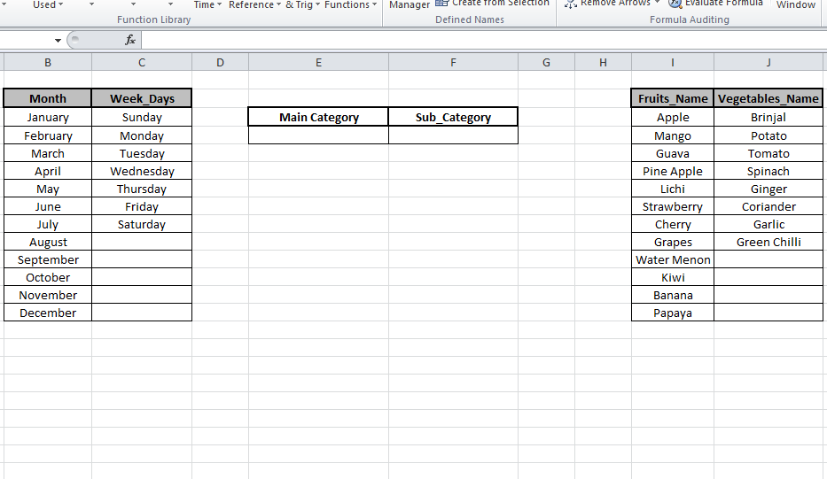
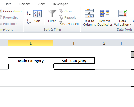
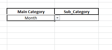
First, we need to create a dropdown list for the Main Category and then we will proceed to Sub_Category.
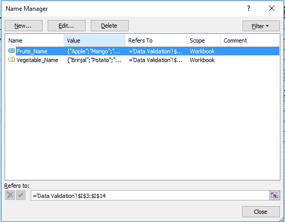
Select Formula>Name Manager in Defined names OR use shortcut Ctrl + F3 to open Name manager where we will keep lists of the array with their names so that we can call them by there name whenever required.
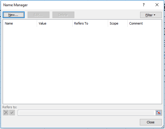
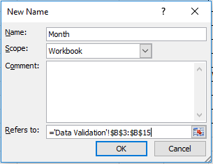
Click New to create. Here Name will be Month and in Refers to option enter the list under Month as shown below.
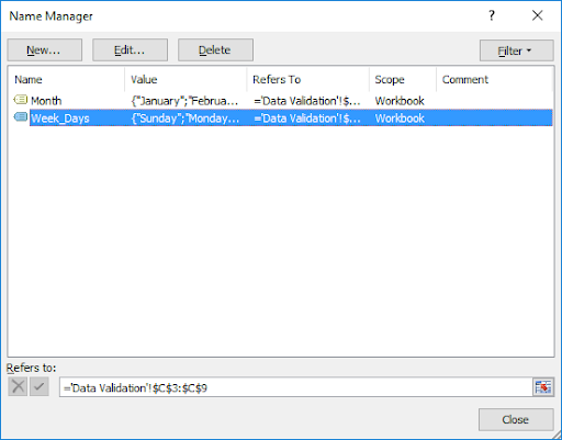
The same we will do for Week_Days and it will show like
Click Close and now select the cell where we need to add dropdown list.
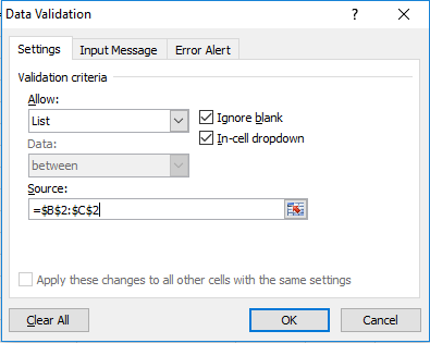
Then Click Data validation under Data bar. Choose list option is Allow and select the cells for main category names which in this case is at B2 and C2 cell “Month” and “Week_Days”
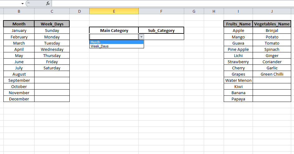
As we can see a drop down list is created which asks the user to choose from the given option.
Now select the cell under Sub_Category and just write the formula in Data validation and click OK.
Formula:

The result is displayed like this

If I don’t want Month and Week_Days. Instead, I want Fruits_Name and vegetables_Name. We just need to edit our Name Manager list.
Press Ctrl + F3 to open Name manager anddelete the already inserted list and add new lists i.e. Fruits_Name and Vegetables_Name.
Instead of Month and Week_Days cell, we will insert Fruits_Name and Vegetables_Name in Data Validation and click OK
Now select the cell under Sub_category as shown in the snapshot below.
Instead of Month and Week_Days cell, we will use Fruits_Name and Vegetables_Name in Data Validation and click OK

As you can see the new list is added here.

This is the way we can edit in the dropdown list and change the list selection.
Below you can find more example:-
How to create drop down list in Excel?
How to delete drop down list in Excel?
How to apply Conditional Formatting in drop down list in Excel?
How to create dependent drop down list in Excel?
How to create multiple dropdown List without repetition using named ranges in Excel?
If you liked our blogs, share it with your friends on Facebook. And also you can follow us on Twitter and Facebook.
We would love to hear from you, do let us know how we can improve, complement or innovate our work and make it better for you. Write us at info@exceltip.com
Popular Articles:
50 Excel Shortcut to Increase Your Productivity
How to use the VLOOKUP Function in Excel
How to use the COUNTIF function in Excel 2016
How to use the SUMIF Function in Excel
Learn how to edit a drop-down list in Excel.
In this blog you will learn how to find, remove and add items to the drop-down list. An extra step is also included for those using older versions of Excel.
How to find items in a drop-down list
Click onto the cell that holds the drop-down list. In this example it is in cell B3.
On the Data tab, select Data Validation.
The Data Validation dialogue box will appear.
The Source information will tell you the source or location of the list. In this example, the drop-down list is coming from the Sales Team worksheet, cells A2 to A13. If at this point the Source information displays just a name, e.g. =salesteam, and not a range, please check the instruction ‘When the drop-down list items are held in a Named Range’ below.
Note: If you can see the list location in the Source box, but cannot see the worksheet where the information is located, it may be because someone has hidden the worksheet. For example, in the image below we cannot see the Sales Team worksheet tab. However we know that the list is in the Sales Team worksheet, therefore it must be hidden.
To check this, right-click the worksheet tabs area and select Unhide.
An Unhide dialogue box will appear, and you will see any hidden worksheets in there.
Select the worksheet you want to unhide an then click OK.
Note: if the worksheet has been protected, you may not be able to unhide it.
When the drop-down list items are held in a Named Range
Sometimes the information shown in the Source box does not look like a range. In the example below, we can only see =SalesTeam in the Source information, and no range.
This is because the list has been saved as a Named range. In this example, the Named range is called SalesTeam.
In order to find its source information, go to the Name box which is on the left of the formula bar.
Click the drop-down arrow at the end of the Name box.
Any Named ranges within the workbook will now be displayed. Click onto the named range you require, e.g. SalesTeam.
And Excel will take you to the location of the Named range. This will be the location of the drop down list items.
Note: If you have not been taken to the list it may be because the worksheet this named range lives in is hidden. If this is the case, follow these steps.
Select the Formulas tab and then Name Manager.
You will see the Named range in the list. The Refers To column will display the location of the Named range. In the example below you can see the Named range is located on the Sales Team worksheet.
Close the Name Manager dialog box and then click on to the worksheet that contains the drop down list menu items.
If the worksheet is hidden, right-click the worksheet tabs and select Unhide to unhide the worksheet and get to the list.
An Unhide dialog box should appear, and you will see any hidden worksheets in there. Select the worksheet you want to unhide.
Click OK.
Note: if the worksheet has been protected, you may not be able to unhide the worksheet.
You can now update information in the drop down items list.
Note: This range is dynamic which means if you update or change names on the original list, this will instantly update the drop-down list. For example, if we changed Able’s name to Abel, this will be updated over in the drop-down list in cell B3.
Remove items from a drop-down list.
Go to the source list. In this example, it is the Sales Team list.
Select the entire row you want to remove.
Right-click and select Delete to remove the entire row.
Note: Make sure to delete the entire row rather than deleting the information in the cells as it prevents you from having a lot of blank spaces in your drop-down list menu.
Add items to drop down list
To add an item to a drop down list, just add it to the list. If you wish to add it between existing items, insert a new row where you would like it included in the list, and then type the item name. For this example, Zander was added to the bottom of the list.
We now need to extend the range for the drop down list items in order to include this new item into the list.
To do this, return to the worksheet with the drop-down list. In this example, this is the ‘Drop down list’ worksheet. Select the cell that contains the drop down list.
Go to the Data tab and select Data Validation.
In the Source box extend your range to include the new item. In this example, we are extending the range from A13 to A14.
Click OK.
You should now have that extra item added to the drop-down list.
Editing drop down items held in a Named range
If your list is held in a Named range, you will not be able to extend the range in the Data Validation box.
Instead, try the following.
Go to the Formulas tab and select Named Manager.
Find the named list and select it.
Select Edit.
The Edit Name dialog box will open. Click into the Refers to box and edit the list range. In the example below we have extended the range from A13 to A14 to include the new list item.
Click OK.
Close the Name Manager dialog box.
You should now have the new item added to the list.
Was this blog helpful? Let us know in the Comments below.
Instructions
How to find the source items in a drop-down list
- Click onto the cell that holds the drop-down list.
- On the Data tab, select Data Validation. The Data Validation dialogue box will appear. The Source information will tell you the source or location of the list.
When the drop-down list items are held in a Named Range
Sometimes the information shown in the Source box does not look like a range. This is because the list has been saved as a Named range.
- Click the drop-down arrow at the end of the Name box (the Name box is located to the left of the Formula Bar. It will display the cell address of the cell that is currently selected).
- Any Named ranges within the workbook will now be displayed. Click onto the Named Range you require. Excel will take you to the location of the Named range. This will be the location of the drop down list items.
Remove items from a drop-down list.
- Go to the source list.
- Select the entire row you want to remove.
- Right-click and select Delete to remove the entire row.
Add items to drop down list
To add an item to a drop down list, just add it to the list. If you wish to add it between existing items, insert a new row where you would like it included in the list, and then type the item name.
To extend the range of the drop down list to include the new item:
- Return to the worksheet that contains the drop-down list. Select the cell or cells that contain the drop down list.
- Go to the Data tab and then select Data Validation.
- In the Source box extend your range to include the new item from the source list.
- Click OK.
Editing drop down items held in a Named range
If your list is held in a Named range, you will not be able to extend the range in the Data Validation box. Instead, try the following.
- Go to the Formulas tab and then select Named Manager.
- Find the Named Range and select it.
- Select Edit. The Edit Name dialog box will open.
- Click into the Refers to box and edit the list range.
- Click OK.
- Close the Name Manager dialog box.
Notes
Note: If you can see the list location in the Source box, but cannot see the worksheet where the information is located, it may be because someone has hidden the worksheet.
Note: This range is dynamic which means if you update or change names on the original list, this will instantly update the drop-down list.
If you enjoyed this post check out the related posts below.
Elevate your Excel game and become a pro with our exclusive Insider Group.
Be the first to know about new tutorials, videos, and tips for Microsoft 365 products. Join us now and claim your exclusive bonus today!
-

1
Open the workbook that contains the drop-down list. Double-clicking the file on your computer will open it in Microsoft Excel.
-
2
Enter additional options for the drop-down list. For this example, we’ll add two new values to a drop-down list in column A. Type each additional option into its own cell at the bottom of the current list.
Advertisement
-
3
Click the Formulas menu. It’s at the top of Excel.
-
4
Click Name Manager. It’s near the center of the ribbon at the top of Excel. A list of named ranges will appear.
-
5
Click the range that contains your drop-down list items.
-
6
Click the upward-pointing arrow button. It’s to the right of the “Refers to” box at the bottom of the Name Manager. This will collapse the Name Manager to a smaller size.
-
7
Select all of the cells in the drop-down menu. Be sure to include the new values you’ve added.
- For example, if the items in your drop-down list are in A2 through A9, highlight A2 through A9.
-
8
Click the downward-pointing button on the Name Manager. It’s at the top of your sheet (the box you collapsed earlier). This re-expands the Name Manager.
-
9
Click Close. A confirmation message will appear.
-
10
Click Yes. The new options you entered are now included in the drop-down menu.


Advertisement
-
1
Open the workbook that contains the drop-down list. Double-clicking the file on your computer will open it in Microsoft Excel.
-
2
Enter additional options for the drop-down list. For this example, we’ll add two new values to a drop-down list in column A. Type each additional option into its own cell at the bottom of the current list.
-
3
Click the Data menu. It’s at the top of the screen.
-
4
Click the drop-down list. It’s the cell at the top of the list that contains a downward-pointing arrow button.
-
5
Click Data validation. It’s in the “Data Tools” group in the ribbon at the top of Excel. This opens the Data Validation window.
-
6
Click the upward-pointing arrow. It’s next to the “Source” field. This collapses the Data Validation window to a smaller size.
-
7
Select the range that contains all items in the list. Be sure to select the old values as well as the ones you just added.
-
8
Click the downward-pointing arrow on the Data Validation window. This is the window you collapsed earlier. The full window will reappear.
-
9
Check the box next to “Apply these changes to all other cells with the same settings.”
-
10
Click OK. Your drop-down menu is now updated.


Advertisement
-
1
Open the workbook that contains the drop-down list. Double-clicking the file on your computer will open it in Microsoft Excel.
- Use this method if your drop-down list is not based on a range of cells, but instead a comma-separated list entered directly into the Data Validation window.
-
2
Click the first cell in the list. This is the cell with the downward-pointing arrow.
-
3
Click the Data menu. It’s at the top of the screen.
-
4
Click Data Validation. It’s in the “Data Tools” section of the ribbon bar at the top of Excel.
-
5
Add or remove items from the “Source” field. Be sure to separate each item with a comma (,).
- Example: Red, Blue, Green, Yellow.
-
6
Check the box next to “Apply these changes to all other cells with the same settings.”
-
7
Click OK. Your drop-down menu is now updated.


Advertisement
Ask a Question
200 characters left
Include your email address to get a message when this question is answered.
Submit
Advertisement
Thanks for submitting a tip for review!
About This Article
Thanks to all authors for creating a page that has been read 29,125 times.