
This tutorial will demonstrate how to drag and drop cells in Excel and Google Sheets.
Drag and drop is a way to copy or move data in Excel using the mouse. It is an alternative to using cut and paste.
The Fill Handle
When you select a cell in Excel, the bottom right-hand corner of the cell contains a small square. This is known as the fill handle. If you click on the fill handle and drag your mouse either down some rows or across some columns, when you let go of the mouse button (drop the cursor), the cells you have dragged over are automatically filled with relevant data.
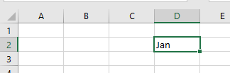
Say you have the value 1 in cell B2. If you click in the bottom right-hand corner of the cell, you will see the fill handle.
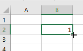
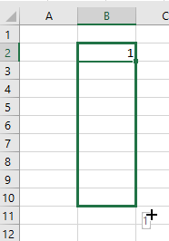
When you rest your mouse on the fill handle, your mouse pointer will change to a small black cross. You can then hold down the mouse button and drag this cross either down the required number of rows, or across the required number of columns.
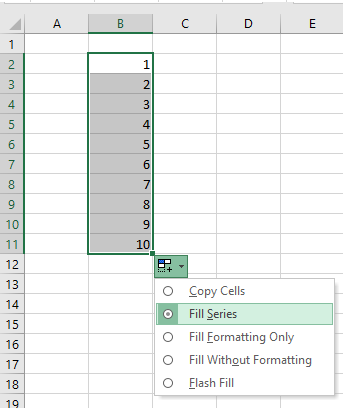
Once you let the mouse button go, the cells you have dragged over are automatically filled, by default, with the value in the first cell (Copy Cells).
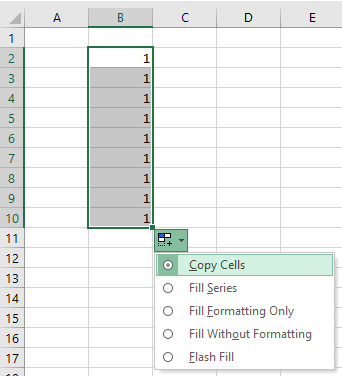
If you want to fill the cells with a series, you can instead select Fill Series.
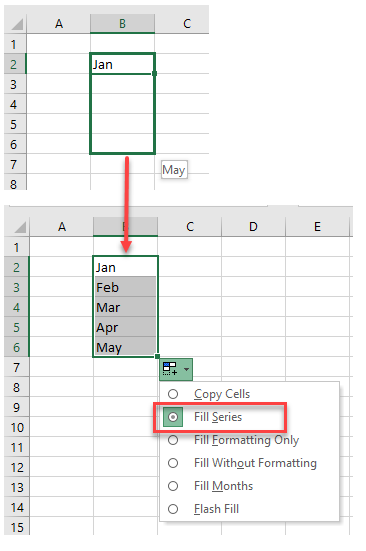
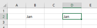
If you have a value in the first cell that is recognized as part of a list, then when you let the mouse go, Excel selects Fill Series to fill with the values from that list.
Move Data From One Cell to Another
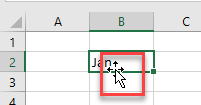
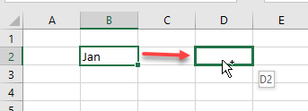
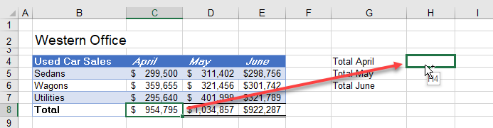
- To move data from one cell to another, select the cell you wish to move and position your mouse at the bottom of the cell. Your mouse pointer will change to an arrow with a small cross.
- Drag the mouse to the cell where you wish to drop the data.
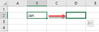
- Release the mouse button to drop the data into the correct cell.
Move Range
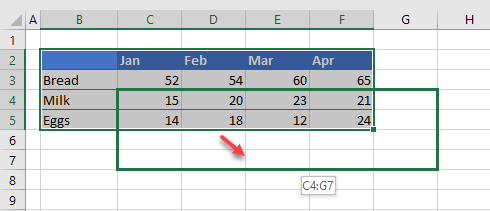
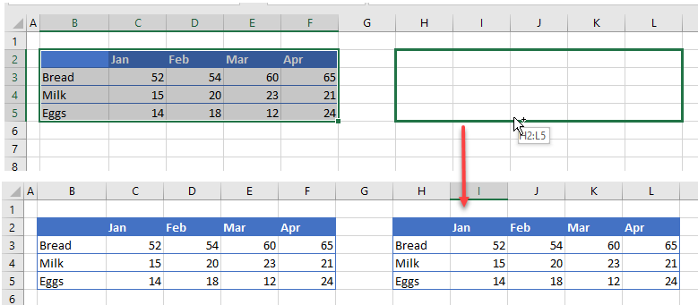
- If you want to move a range of cells, select all the cells you wish to move, and then move your mouse to the bottom row in the selection. Your mouse pointer will change to an arrow with a small white cross attached to it.
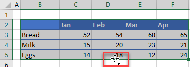
- Drag the mouse across or down to where you wish the cells to be moved to.
- Release the mouse cursor to drop the cells into the correct position.

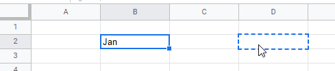
Copy Data From One Cell to Another
Copying cell data by drag and drop is similar to moving cell data explained above except when you drag the mouse, hold the CTRL key down on the keyboard.
- Select the cell you wish to copy and position your mouse at the bottom of the cell. Hold down CTRL and notice the mouse pointer now has a small plus sign.
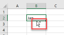
- Still holding down the CTRL key, drag the mouse across to the destination cell.
- Release the mouse button to copy the cell data.
This can of course, like moving the cell data, be down on a range of cells.
Drag and Drop Over Existing Data
If there is already data in the destination cell or cells where you are dragging the data to, Excel warns you about over writing the data that already exists.
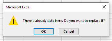
Click OK to replace the data with the new data or Cancel to stop the drag and drop.
Drag and Drop Formulas
Fill Handle
You can use the fill handle to drag and drop dynamic formulas.
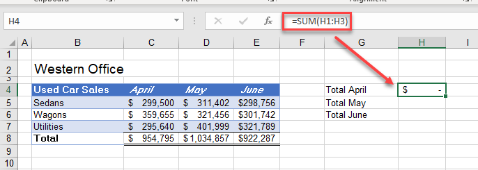
- Select the cell that contains the formula you wish to copy, and then move your mouse pointer to the fill handle on the right-hand side of the cell.
- Drag the fill handle across the cells where you wish the formula to be copied to.
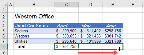
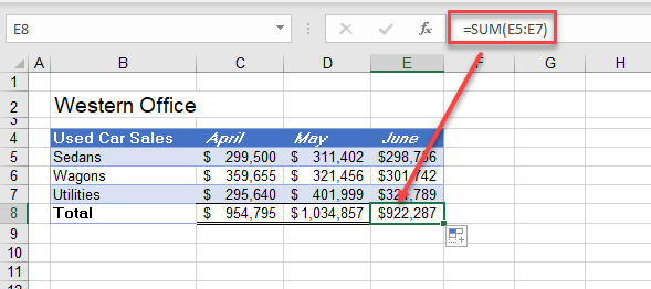
- Release the mouse button to drop the formulas into the selected cells. Notice that the formula changes dynamically as it is dragged across to its destination cells.
Move Formula
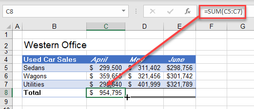
To move a formula using drag and drop, position your mouse at the bottom of the cell, and then drag the formula to your desired position
The formula doesn’t change dynamically but is moved to the destination location.
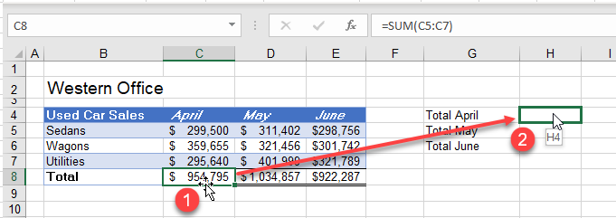
To copy the formula rather than move the formula, hold down the CTRL key as you drag the mouse across to the destination location.
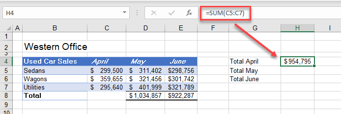
Notice that when you drag and drop a formula using this method, the formula does change dynamically.
Drag and Drop Cells in Google Sheets
Dragging and dropping cells and formulas in Google Sheets works similarly.
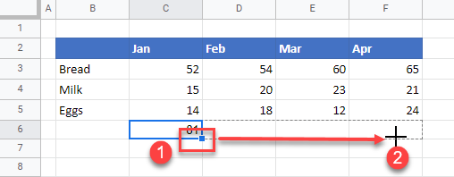
To drag a formula across, select the fill handle, and then drag across to the final cell in your destination range.
To move data or a formula, select the cell where the data or formula is. Your mouse pointer should change to a small hand icon.
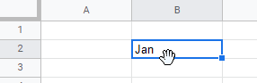
Drag the data or formula to its destination cell and release the mouse.
One limitation with Google Sheets is you cannot copy a formula (to a nonadjacent cell) using drag and drop. You would have to use CTRL + C and CTRL + V to copy formulas from one cell to another.
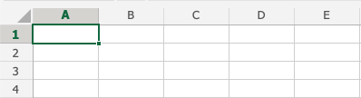
Delete Cells
Cells can be deleted by selecting them, and pressing the delete button.
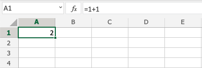
Note: The delete function will not delete the formatting of the cell, just the value inside of it.
Let’s have a look at three examples.
Example 1
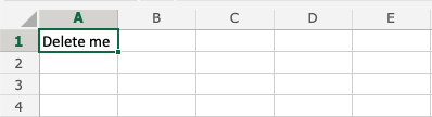
Pressing the delete button:
Example 2
Pressing the delete button:
Example 3
With formatting:
Pressing the delete button:
Note that it only deletes the value in the cells, and not the formatting (the color).
Note: You will learn more about formatting, and how to style cells in a later chapter.
Test Yourself With Exercises
Move or copy cells and cell contents
Use Cut, Copy, and Paste to move or copy cell contents. Or copy specific contents or attributes from the cells. For example, copy the resulting value of a formula without copying the formula, or copy only the formula.
When you move or copy a cell, Excel moves or copies the cell, including formulas and their resulting values, cell formats, and comments.
You can move cells in Excel by drag and dropping or using the Cut and Paste commands.

Move cells by drag and dropping
-
Select the cells or range of cells that you want to move or copy.
-
Point to the border of the selection.
-
When the pointer becomes a move pointer
 , drag the cell or range of cells to another location.
 , drag the cell or range of cells to another location.
Move cells by using Cut and Paste
-
Select a cell or a cell range.
-
Select Home > Cut
or press Ctrl + X. -
Select a cell where you want to move the data.
-
Select Home > Paste
or press Ctrl + V.
 or press Ctrl + X.
 or press Ctrl + V.
Copy cells by using Copy and Paste
-
Select the cell or range of cells.
-
Select Copy or press Ctrl + C.
-
Select Paste or press Ctrl + V.
Need more help?
You can always ask an expert in the Excel Tech Community or get support in the Answers community.
See Also
Move or copy cells, rows, and columns
Need more help?
If you later decide you no longer need a group of cells, columns, or rows, you can delete them. Deleting a cell differs from clearing a cell’s content, as a “hole” is created by the deleted cell(s) and adjacent cells will move to fill that hole.
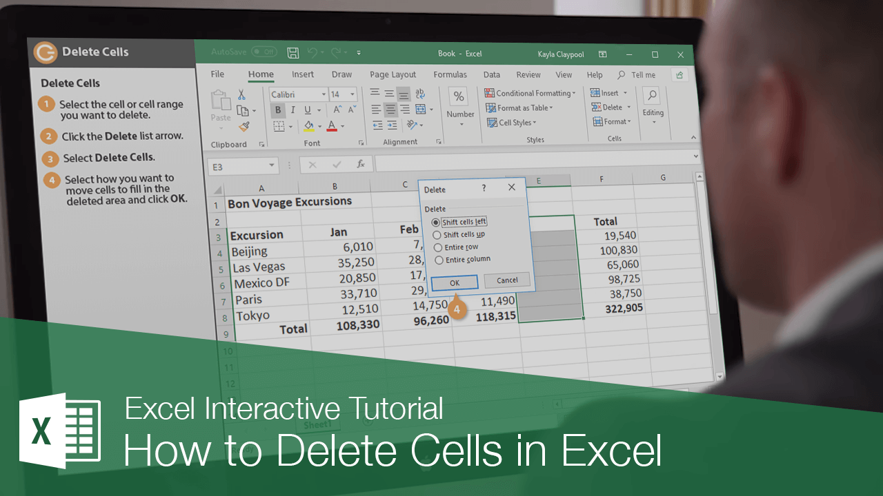
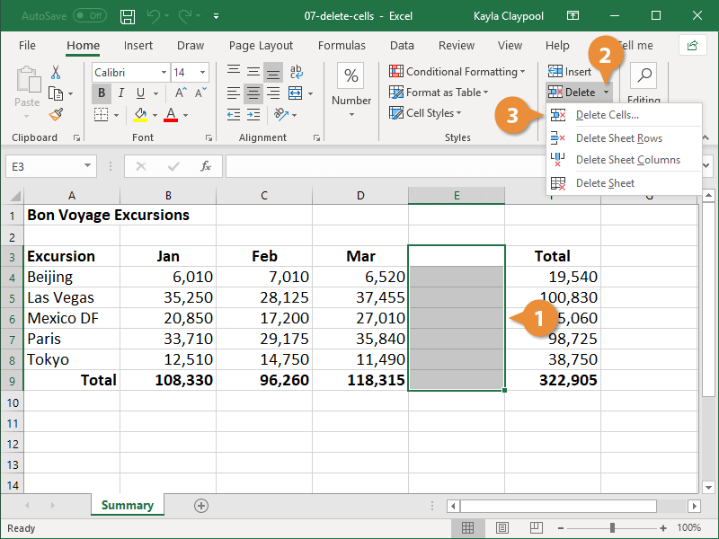
Delete Cells
- Select the cell or cell range where you want to delete.
- Click the Delete list arrow.
- Select Delete Cells.

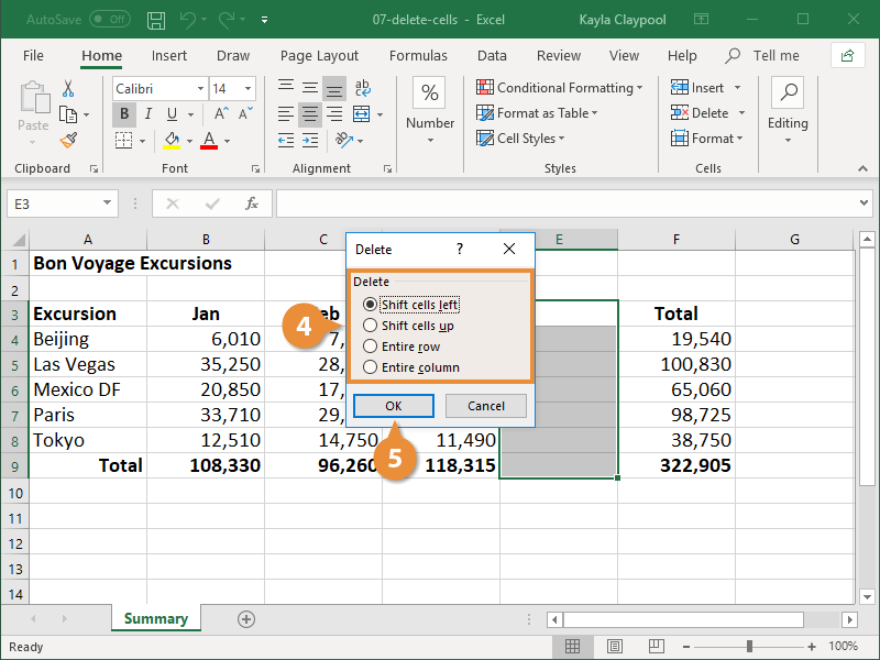
The Delete dialog box appears.
- Select how you want to move cells to fill in the deleted area:
- Shift cells right: Shift existing cells to the right.
- Shift cells down: Shift existing cells down.
- Entire row: Delete an entire row.
- Entire column: Delete an entire column.
- Click OK.
You can also delete cells by right-clicking the selected cell(s) and selecting Delete from the contextual menu.
Pressing the Delete key only clears a cell’s contents; it doesn’t delete the actual cell.
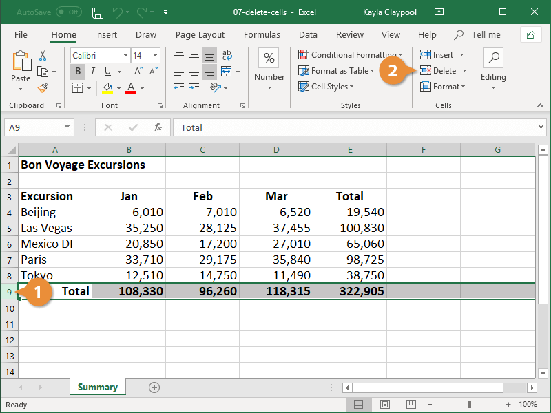
The cell(s) are deleted and the remaining cells are shifted.
Delete Rows or Columns
- Select the column or row you want to delete.
- Click the Delete button.
You can also delete cells by right-clicking the selected cell(s) and selecting Delete from the contextual menu.
The rows or columns are deleted. Remaining rows are shifted up, while remaining columns are shifted to the left.

FREE Quick Reference
Click to Download
Free to distribute with our compliments; we hope you will consider our paid training.
Содержание
- Add or remove items from a drop-down list
- Edit a drop-down list that’s based on an Excel Table
- Edit a drop-down list that’s based on an Excel Table
- Need more help?
- How to Create a Drop Down List in Excel (the Only Guide You Need)
- How to Create a Drop Down List in Excel
- #1 Using Data from Cells
- #2 By Entering Data Manually
- #3 Using Excel Formulas
- Creating a Dynamic Drop Down List in Excel (Using OFFSET)
- Copy Pasting Drop-Down Lists in Excel
- Caution while Working with Excel Drop Down List
- How to Select All Cells that have a Drop Down List in it
- Creating a Dependent / Conditional Excel Drop Down List
Add or remove items from a drop-down list
After you create a drop-down list, you might want to add more items or delete items. In this article, we’ll show you how to do that depending on how the list was created.
Edit a drop-down list that’s based on an Excel Table
If you set up your list source as an Excel table, then all you need to do is add or remove items from the list, and Excel will automatically update any associated drop-downs for you.
To add an item, go to the end of the list and type the new item.
To remove an item, press Delete.
Tip: If the item you want to delete is somewhere in the middle of your list, right-click its cell, click Delete, and then click OK to shift the cells up.
Select the worksheet that has the named range for your drop-down list.
Do any of the following:
To add an item, go to the end of the list and type the new item.
To remove an item, press Delete.
Tip: If the item you want to delete is somewhere in the middle of your list, right-click its cell, click Delete, and then click OK to shift the cells up.
Go to Formulas > Name Manager.
In the Name Manager box, click the named range you want to update.
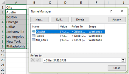
Click in the Refers to box, and then on your worksheet select all of the cells that contain the entries for your drop-down list.
Click Close, and then click Yes to save your changes.
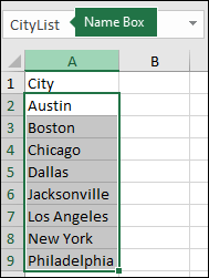
Tip: If you don’t know what a named range is named, you can select the range and look for its name in the Name Box. To locate a named range, see Find named ranges.
Select the worksheet that has the data for your drop-down list.
Do any of the following:
To add an item, go to the end of the list and type the new item.
To remove an item, click Delete.
Tip: If the item you want to delete is somewhere in the middle of your list, right-click its cell, click Delete, and then click OK to shift the cells up.
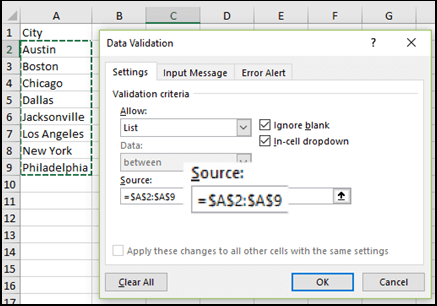
On the worksheet where you applied the drop-down list, select a cell that has the drop-down list.
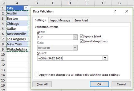
Go to Data > Data Validation.
On the Settings tab, click in the Source box, and then on the worksheet that has the entries for your drop-down list, select all of the cells containing those entries. You’ll see the list range in the Source box change as you select.
To update all cells that have the same drop-down list applied, check the Apply these changes to all other cells with the same settings box.
On the worksheet where you applied the drop-down list, select a cell that has the drop-down list.
Go to Data > Data Validation.
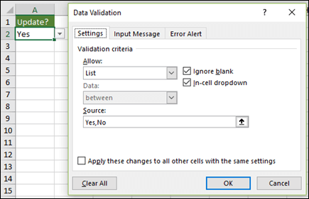
On the Settings tab, click in the Source box, and then change your list items as needed. Each item should be separated by a comma, with no spaces in between like this: Yes,No,Maybe.
To update all cells that have the same drop-down list applied, check the Apply these changes to all other cells with the same settings box.
After you update a drop-down list, make sure it works the way you want. For example, check to see if the cell is wide enough to show your updated entries.
If the list of entries for your drop-down list is on another worksheet and you want to prevent users from seeing it or making changes, consider hiding and protecting that worksheet. For more information about how to protect a worksheet, see Lock cells to protect them.
If you want to delete your drop-down list, see Remove a drop-down list.
To see a video about how to work with drop-down lists, see Create and manage drop-down lists.
Edit a drop-down list that’s based on an Excel Table
If you set up your list source as an Excel table, then all you need to do is add or remove items from the list, and Excel will automatically update any associated drop-downs for you.
To add an item, go to the end of the list and type the new item.
To remove an item, press Delete.
Tip: If the item you want to delete is somewhere in the middle of your list, right-click its cell, click Delete, and then click OK to shift the cells up.
Select the worksheet that has the named range for your drop-down list.
Do any of the following:
To add an item, go to the end of the list and type the new item.
To remove an item, press Delete.
Tip: If the item you want to delete is somewhere in the middle of your list, right-click its cell, click Delete, and then click OK to shift the cells up.
Go to Formulas > Name Manager.
In the Name Manager box, click the named range you want to update.
Click in the Refers to box, and then on your worksheet select all of the cells that contain the entries for your drop-down list.
Click Close, and then click Yes to save your changes.
Tip: If you don’t know what a named range is named, you can select the range and look for its name in the Name Box. To locate a named range, see Find named ranges.
Select the worksheet that has the data for your drop-down list.
Do any of the following:
To add an item, go to the end of the list and type the new item.
To remove an item, click Delete.
Tip: If the item you want to delete is somewhere in the middle of your list, right-click its cell, click Delete, and then click OK to shift the cells up.
On the worksheet where you applied the drop-down list, select a cell that has the drop-down list.
Go to Data > Data Validation.
On the Settings tab, click in the Source box, and then on the worksheet that has the entries for your drop-down list, Select cell contents in Excel containing those entries. You’ll see the list range in the Source box change as you select.
To update all cells that have the same drop-down list applied, check the Apply these changes to all other cells with the same settings box.
On the worksheet where you applied the drop-down list, select a cell that has the drop-down list.
Go to Data > Data Validation.
On the Settings tab, click in the Source box, and then change your list items as needed. Each item should be separated by a comma, with no spaces in between like this: Yes,No,Maybe.
To update all cells that have the same drop-down list applied, check the Apply these changes to all other cells with the same settings box.
After you update a drop-down list, make sure it works the way you want. For example, check to see how to Change the column width and row height to show your updated entries.
If the list of entries for your drop-down list is on another worksheet and you want to prevent users from seeing it or making changes, consider hiding and protecting that worksheet. For more information about how to protect a worksheet, see Lock cells to protect them.
If you want to delete your drop-down list, see Remove a drop-down list.
To see a video about how to work with drop-down lists, see Create and manage drop-down lists.
In Excel for the web, you can only edit a drop-down list where the source data has been entered manually.
Select the cells that have the drop-down list.
Go to Data > Data Validation.
On the Settings tab, click in the Source box. Then do one of the following:
If the Source box contains drop-down entries separated by commas, then type new entries or remove ones you don’t need. When you’re done, each entry should be separated by a comma, with no spaces. For example: Fruits,Vegetables,Meat,Deli.
If the Source box contains a reference to a range of cells (for example, =$A$2:$A$5), click Cancel, and then add or remove entries from those cells. In this example, you’d add or remove entries in cells A2 through A5. If the list of entries ends up being longer or shorter than the original range, go back to the Settings tab and delete what’s in the Source box. Then click and drag to select the new range containing the entries.
If the Source box contains a named range, like Departments, then you need to change the range itself using a desktop version of Excel.
After you update a drop-down list, make sure it works the way you want. For example, check to see if the cell is wide enough to show your updated entries. If you want to delete your drop-down list, see Remove a drop-down list.
Need more help?
You can always ask an expert in the Excel Tech Community or get support in the Answers community.
Источник
How to Create a Drop Down List in Excel (the Only Guide You Need)
A drop-down list is an excellent way to give the user an option to select from a pre-defined list.
It can be used while getting a user to fill a form, or while creating interactive Excel dashboards.
Drop-down lists are quite common on websites/apps and are very intuitive for the user.
Watch Video – Creating a Drop Down List in Excel
In this tutorial, you’ll learn how to create a drop down list in Excel (it takes only a few seconds to do this) along with all the awesome stuff you can do with it.
This Tutorial Covers:
How to Create a Drop Down List in Excel
In this section, you will learn the exacts steps to create an Excel drop-down list:
- Using Data from Cells.
- Entering Data Manually.
- Using the OFFSET formula.
#1 Using Data from Cells
Let’s say you have a list of items as shown below:
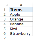
Here are the steps to create an Excel Drop Down List:
- Select a cell where you want to create the drop down list.
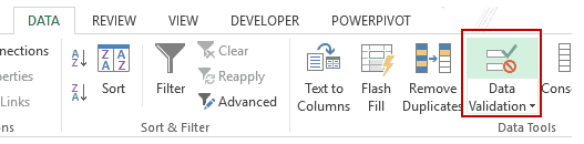
- Go to Data –> Data Tools –> Data Validation.
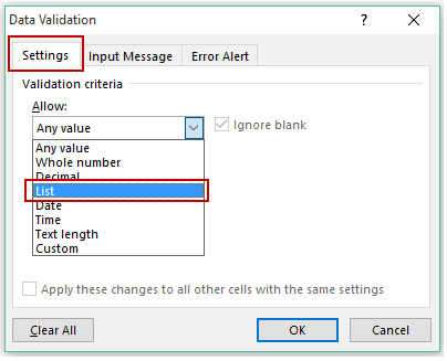
- In the Data Validation dialogue box, within the Settings tab, select List as the Validation criteria.
- As soon as you select List, the source field appears.
- As soon as you select List, the source field appears.
- In the source field, enter =$A$2:$A$6 , or simply click in the Source field and select the cells using the mouse and click OK. This will insert a drop down list in cell C2.
- Make sure that the In-cell dropdown option is checked (which is checked by default). If this option in unchecked, the cell does not show a drop down, however, you can manually enter the values in the list.
- Make sure that the In-cell dropdown option is checked (which is checked by default). If this option in unchecked, the cell does not show a drop down, however, you can manually enter the values in the list.
Note: If you want to create drop down lists in multiple cells at one go, select all the cells where you want to create it and then follow the above steps. Make sure that the cell references are absolute (such as $A$2) and not relative (such as A2, or A$2, or $A2).
#2 By Entering Data Manually
In the above example, cell references are used in the Source field. You can also add items directly by entering it manually in the source field.
For example, let’s say you want to show two options, Yes and No, in the drop down in a cell. Here is how you can directly enter it in the data validation source field:
This will create a drop-down list in the selected cell. All the items listed in the source field, separated by a comma, are listed in different lines in the drop down menu.
All the items entered in the source field, separated by a comma, are displayed in different lines in the drop down list.
Note: If you want to create drop down lists in multiple cells at one go, select all the cells where you want to create it and then follow the above steps.
#3 Using Excel Formulas
Apart from selecting from cells and entering data manually, you can also use a formula in the source field to create an Excel drop down list.
Any formula that returns a list of values can be used to create a drop-down list in Excel.
For example, suppose you have the data set as shown below:
Here are the steps to create an Excel drop down list using the OFFSET function:
This will create a drop-down list that lists all the fruit names (as shown below).
 Note : If you want to create a drop-down list in multiple cells at one go, select all the cells where you want to create it and then follow the above steps. Make sure that the cell references are absolute (such as $A$2) and not relative (such as A2, or A$2, or $A2).
How this formula Works??
In the above case, we used an OFFSET function to create the drop down list. It returns a list of items from the ra
It returns a list of items from the range A2:A6.
Here is the syntax of the OFFSET function: =OFFSET(reference, rows, cols, [height], [width])
It takes five arguments, where we specified the reference as A2 (the starting point of the list). Rows/Cols are specified as 0 as we don’t want to offset the reference cell. Height is specified as 5 as there are five elements in the list.
Now, when you use this formula, it returns an array that has the list of the five fruits in A2:A6. Note that if you enter the formula in a cell, select it and press F9, you would see that it returns an array of the fruit names.
Creating a Dynamic Drop Down List in Excel (Using OFFSET)
The above technique of using a formula to create a drop down list can be extended to create a dynamic drop down list as well. If you use the OFFSET function, as shown above, even if you add more items to the list, the drop down would not update automatically. You will have to manually update it each time you change the list.
Here is a way to make it dynamic (and it’s nothing but a minor tweak in the formula):
- Select a cell where you want to create the drop down list (cell C2 in this example).
- Go to Data –> Data Tools –> Data Validation.
- In the Data Validation dialogue box, within the Settings tab, select List as the Validation criteria. As soon as you select List, the source field appears.
- In the source field, enter the following formula: =OFFSET($A$2,0,0,COUNTIF($A$2:$A$100,”<>”))
- Make sure that the In-cell drop down option is checked.
- Click OK.
In this formula, I have replaced the argument 5 with COUNTIF($A$2:$A$100,”<>”).
The COUNTIF function counts the non-blank cells in the range A2:A100. Hence, the OFFSET function adjusts itself to include all the non-blank cells.
Note:
- For this to work, there must NOT be any blank cells in between the cells that are filled.
- If you want to create a drop-down list in multiple cells at one go, select all the cells where you want to create it and then follow the above steps. Make sure that the cell references are absolute (such as $A$2) and not relative (such as A2, or A$2, or $A2).
Copy Pasting Drop-Down Lists in Excel
You can copy paste the cells with data validation to other cells, and it will copy the data validation as well.
For example, if you have a drop-down list in cell C2, and you want to apply it to C3:C6 as well, simply copy the cell C2 and paste it in C3:C6. This will copy the drop-down list and make it available in C3:C6 (along with the drop down, it will also copy the formatting).
If you only want to copy the drop down and not the formatting, here are the steps:
This will only copy the drop down and not the formatting of the copied cell.
Caution while Working with Excel Drop Down List
You need to to be careful when you are working with drop down lists in Excel.
When you copy a cell (that does not contain a drop down list) over a cell that contains a drop down list, the drop down list is lost.
The worst part of this is that Excel will not show any alert or prompt to let the user know that a drop down will be overwritten.
How to Select All Cells that have a Drop Down List in it
Sometimes, it ‘s hard to know which cells contain the drop down list.
Hence, it makes sense to mark these cells by either giving it a distinct border or a background color.
Instead of manually checking all the cells, there is a quick way to select all the cells that have drop-down lists (or any data validation rule) in it.
This would instantly select all the cells that have a data validation rule applied to it (this includes drop down lists as well).
Now you can simply format the cells (give a border or a background color) so that visually visible and you don’t accidentally copy another cell on it.
Here is another technique by Jon Acampora you can use to always keep the drop down arrow icon visible. You can also see some ways to do this in this video by Mr. Excel.
Creating a Dependent / Conditional Excel Drop Down List
Here is a video on how to create a dependent drop-down list in Excel.
If you prefer reading over watching a video, keep reading.
Sometimes, you may have more than one drop-down list and you want the items displayed in the second drop down to be dependent on what the user selected in the first drop-down.
These are called dependent or conditional drop down lists.
Below is an example of a conditional/dependent drop down list:

In the above example, when the items listed in ‘Drop Down 2’ are dependent on the selection made in ‘Drop Down 1’.
Now let’s see how to create this.
Here are the steps to create a dependent / conditional drop down list in Excel:
Now, when you make the selection in Drop Down 1, the options listed in Drop Down List 2 would automatically update.
Download the Example File 
How does this work? – The conditional drop down list (in cell E3) refers to =INDIRECT(D3). This means that when you select ‘Fruits’ in cell D3, the drop down list in E3 refers to the named range ‘Fruits’ (through the INDIRECT function) and hence lists all the items in that category.
Important Note While Working with Conditional Drop Down Lists in Excel:
- When you have made the selection, and then you change the parent drop down, the dependent drop down would not change and would, therefore, be a wrong entry. For example, if you select the US as the country and then select Florida as the state, and then go back and change the country to India, the state would remain as Florida. Here is a great tutorial by Debra on clearing dependent (conditional) drop down lists in Excel when the selection is changed.
- If the main category is more than one word (for example, ‘Seasonal Fruits’ instead of ‘Fruits’), then you need to use the formula =INDIRECT(SUBSTITUTE(D3,” “,”_”)), instead of the simple INDIRECT function shown above. The reason for this is that Excel does not allow spaces in named ranges. So when you create a named range using more than one word, Excel automatically inserts an underscore in between words. So ‘Seasonal Fruits’ named range would be ‘Seasonal_Fruits’. Using the SUBSTITUTE function within the INDIRECT function makes sure that spaces are converted into underscores.
You May Also Like the Following Excel Tutorials:
Источник