
Abstract: This is the first tutorial in a series designed to get you acquainted and comfortable using Excel and its built-in data mash-up and analysis features. These tutorials build and refine an Excel workbook from scratch, build a data model, then create amazing interactive reports using Power View. The tutorials are designed to demonstrate Microsoft Business Intelligence features and capabilities in Excel, PivotTables, Power Pivot, and Power View.
Note: This article describes data models in Excel 2013. However, the same data modeling and Power Pivot features introduced in Excel 2013 also apply to Excel 2016.
In these tutorials you learn how to import and explore data in Excel, build and refine a data model using Power Pivot, and create interactive reports with Power View that you can publish, protect, and share.
The tutorials in this series are the following:
-
Import Data into Excel 2013, and Create a Data Model
-
Extend Data Model relationships using Excel, Power Pivot, and DAX
-
Create Map-based Power View Reports
-
Incorporate Internet Data, and Set Power View Report Defaults
-
Power Pivot Help
-
Create Amazing Power View Reports — Part 2
In this tutorial, you start with a blank Excel workbook.
The sections in this tutorial are the following:
-
Import data from a database
-
Import data from a spreadsheet
-
Import data using copy and paste
-
Create a relationship between imported data
-
Checkpoint and Quiz
At the end of this tutorial is a quiz you can take to test your learning.
This tutorial series uses data describing Olympic Medals, hosting countries, and various Olympic sporting events. We suggest you go through each tutorial in order. Also, tutorials use Excel 2013 with Power Pivot enabled. For more information on Excel 2013, click here. For guidance on enabling Power Pivot, click here.
Import data from a database
We start this tutorial with a blank workbook. The goal in this section is to connect to an external data source, and import that data into Excel for further analysis.
Let’s start by downloading some data from the Internet. The data describes Olympic Medals, and is a Microsoft Access database.
-
Click the following links to download files we use during this tutorial series. Download each of the four files to a location that’s easily accessible, such as Downloads or My Documents, or to a new folder you create:
> OlympicMedals.accdb Access database
> OlympicSports.xlsx Excel workbook
> Population.xlsx Excel workbook
> DiscImage_table.xlsx Excel workbook -
In Excel 2013, open a blank workbook.
-
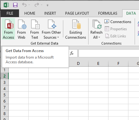
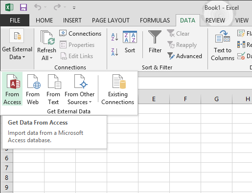
Click DATA > Get External Data > From Access. The ribbon adjusts dynamically based on the width of your workbook, so the commands on your ribbon may look slightly different from the following screens. The first screen shows the ribbon when a workbook is wide, the second image shows a workbook that has been resized to take up only a portion of the screen.

-
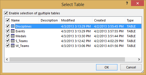
Select the OlympicMedals.accdb file you downloaded and click Open. The following Select Table window appears, displaying the tables found in the database. Tables in a database are similar to worksheets or tables in Excel. Check the Enable selection of multiple tables box, and select all the tables. Then click OK.
-
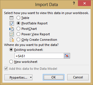
The Import Data window appears.
Note: Notice the checkbox at the bottom of the window that allows you to Add this data to the Data Model, shown in the following screen. A Data Model is created automatically when you import or work with two or more tables simultaneously. A Data Model integrates the tables, enabling extensive analysis using PivotTables, Power Pivot, and Power View. When you import tables from a database, the existing database relationships between those tables is used to create the Data Model in Excel. The Data Model is transparent in Excel, but you can view and modify it directly using the Power Pivot add-in. The Data Model is discussed in more detail later in this tutorial.
Select the PivotTable Report option, which imports the tables into Excel and prepares a PivotTable for analyzing the imported tables, and click OK.
-
Once the data is imported, a PivotTable is created using the imported tables.
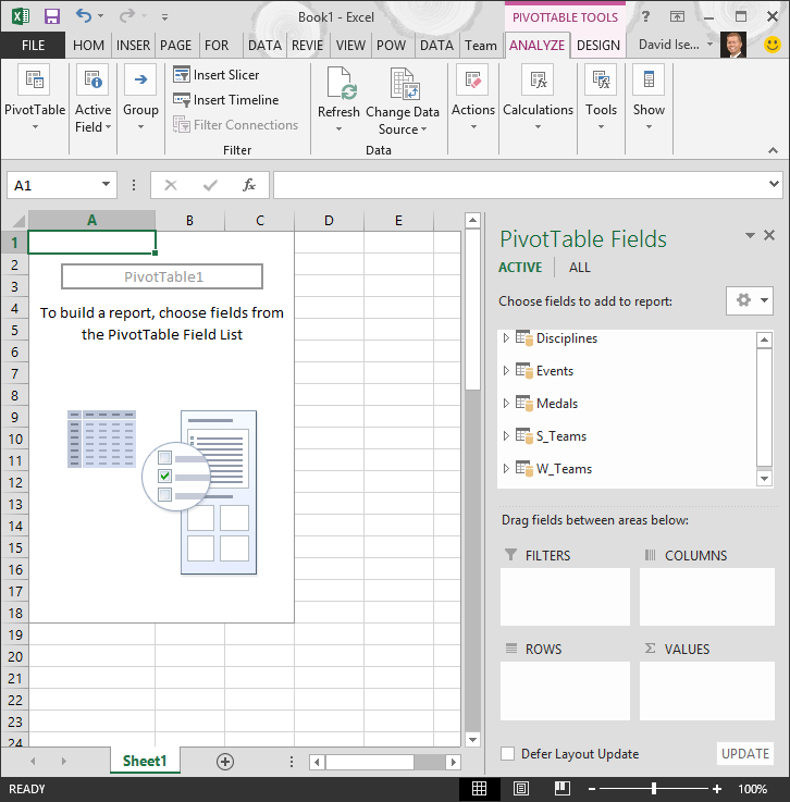
With the data imported into Excel, and the Data Model automatically created, you’re ready to explore the data.
Explore data using a PivotTable
Exploring imported data is easy using a PivotTable. In a PivotTable, you drag fields (similar to columns in Excel) from tables (like the tables you just imported from the Access database) into different areas of the PivotTable to adjust how it presents your data. A PivotTable has four areas: FILTERS, COLUMNS, ROWS, and VALUES.
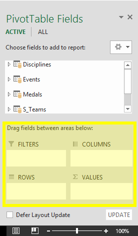
It might take some experimenting to determine which area a field should be dragged to. You can drag as many or few fields from your tables as you like, until the PivotTable presents your data how you want to see it. Feel free to explore by dragging fields into different areas of the PivotTable; the underlying data is not affected when you arrange fields in a PivotTable.
Let’s explore the Olympic Medals data in the PivotTable, starting with Olympic medalists organized by discipline, medal type, and the athlete’s country or region.
-
In PivotTable Fields, expand the Medals table by clicking the arrow beside it. Find the NOC_CountryRegion field in the expanded Medals table, and drag it to the COLUMNS area. NOC stands for National Olympic Committees, which is the organizational unit for a country or region.
-
Next, from the Disciplines table, drag Discipline to the ROWS area.
-
Let’s filter Disciplines to display only five sports: Archery, Diving, Fencing, Figure Skating, and Speed Skating. You can do this from within the PivotTable Fields area, or from the Row Labels filter in the PivotTable itself.
-
Click anywhere in the PivotTable to ensure the Excel PivotTable is selected. In the PivotTable Fields list, where the Disciplines table is expanded, hover over its Discipline field and a dropdown arrow appears to the right of the field. Click the dropdown, click (Select All)to remove all selections, then scroll down and select Archery, Diving, Fencing, Figure Skating, and Speed Skating. Click OK.
-
Or, in the Row Labels section of the PivotTable, click the dropdown next to Row Labels in the PivotTable, click (Select All) to remove all selections, then scroll down and select Archery, Diving, Fencing, Figure Skating, and Speed Skating. Click OK.
-
-
In PivotTable Fields, from the Medals table, drag Medal to the VALUES area. Since Values must be numeric, Excel automatically changes Medal to Count of Medal.
-
From the Medals table, select Medal again and drag it into the FILTERS area.
-
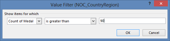
Let’s filter the PivotTable to display only those countries or regions with more than 90 total medals. Here’s how.
-
In the PivotTable, click the dropdown to the right of Column Labels.
-
Select Value Filters and select Greater Than….
-
Type 90 in the last field (on the right). Click OK.
-
Your PivotTable looks like the following screen.
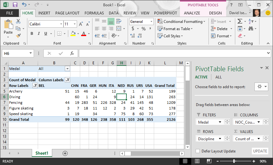
With little effort, you now have a basic PivotTable that includes fields from three different tables. What made this task so simple were the pre-existing relationships among the tables. Because table relationships existed in the source database, and because you imported all the tables in a single operation, Excel could recreate those table relationships in its Data Model.
But what if your data originates from different sources, or is imported at a later time? Typically, you can create relationships with new data based on matching columns. In the next step, you import additional tables, and learn how to create new relationships.
Import data from a spreadsheet
Now let’s import data from another source, this time from an existing workbook, then specify the relationships between our existing data and the new data. Relationships let you analyze collections of data in Excel, and create interesting and immersive visualizations from the data you import.
Let’s start by creating a blank worksheet, then import data from an Excel workbook.
-
Insert a new Excel worksheet, and name it Sports.
-
Browse to the folder that contains the downloaded sample data files, and open OlympicSports.xlsx.
-
Select and copy the data in Sheet1. If you select a cell with data, such as cell A1, you can press Ctrl + A to select all adjacent data. Close the OlympicSports.xlsx workbook.
-
On the Sports worksheet, place your cursor in cell A1 and paste the data.
-
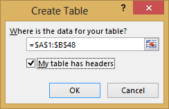
With the data still highlighted, press Ctrl + T to format the data as a table. You can also format the data as a table from the ribbon by selecting HOME > Format as Table. Since the data has headers, select My table has headers in the Create Table window that appears, as shown here.
Formatting the data as a table has many advantages. You can assign a name to a table, which makes it easy to identify. You can also establish relationships between tables, enabling exploration and analysis in PivotTables, Power Pivot, and Power View.
-
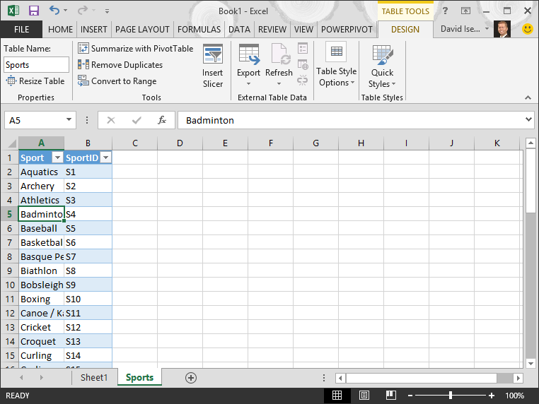
Name the table. In TABLE TOOLS > DESIGN > Properties, locate the Table Name field and type Sports. The workbook looks like the following screen.
-
Save the workbook.
Import data using copy and paste
Now that we’ve imported data from an Excel workbook, let’s import data from a table we find on a web page, or any other source from which we can copy and paste into Excel. In the following steps, you add the Olympic host cities from a table.
-
Insert a new Excel worksheet, and name it Hosts.
-
Select and copy the following table, including the table headers.
|
City |
NOC_CountryRegion |
Alpha-2 Code |
Edition |
Season |
|
Melbourne / Stockholm |
AUS |
AS |
1956 |
Summer |
|
Sydney |
AUS |
AS |
2000 |
Summer |
|
Innsbruck |
AUT |
AT |
1964 |
Winter |
|
Innsbruck |
AUT |
AT |
1976 |
Winter |
|
Antwerp |
BEL |
BE |
1920 |
Summer |
|
Antwerp |
BEL |
BE |
1920 |
Winter |
|
Montreal |
CAN |
CA |
1976 |
Summer |
|
Lake Placid |
CAN |
CA |
1980 |
Winter |
|
Calgary |
CAN |
CA |
1988 |
Winter |
|
St. Moritz |
SUI |
SZ |
1928 |
Winter |
|
St. Moritz |
SUI |
SZ |
1948 |
Winter |
|
Beijing |
CHN |
CH |
2008 |
Summer |
|
Berlin |
GER |
GM |
1936 |
Summer |
|
Garmisch-Partenkirchen |
GER |
GM |
1936 |
Winter |
|
Barcelona |
ESP |
SP |
1992 |
Summer |
|
Helsinki |
FIN |
FI |
1952 |
Summer |
|
Paris |
FRA |
FR |
1900 |
Summer |
|
Paris |
FRA |
FR |
1924 |
Summer |
|
Chamonix |
FRA |
FR |
1924 |
Winter |
|
Grenoble |
FRA |
FR |
1968 |
Winter |
|
Albertville |
FRA |
FR |
1992 |
Winter |
|
London |
GBR |
UK |
1908 |
Summer |
|
London |
GBR |
UK |
1908 |
Winter |
|
London |
GBR |
UK |
1948 |
Summer |
|
Munich |
GER |
DE |
1972 |
Summer |
|
Athens |
GRC |
GR |
2004 |
Summer |
|
Cortina d’Ampezzo |
ITA |
IT |
1956 |
Winter |
|
Rome |
ITA |
IT |
1960 |
Summer |
|
Turin |
ITA |
IT |
2006 |
Winter |
|
Tokyo |
JPN |
JA |
1964 |
Summer |
|
Sapporo |
JPN |
JA |
1972 |
Winter |
|
Nagano |
JPN |
JA |
1998 |
Winter |
|
Seoul |
KOR |
KS |
1988 |
Summer |
|
Mexico |
MEX |
MX |
1968 |
Summer |
|
Amsterdam |
NED |
NL |
1928 |
Summer |
|
Oslo |
NOR |
NO |
1952 |
Winter |
|
Lillehammer |
NOR |
NO |
1994 |
Winter |
|
Stockholm |
SWE |
SW |
1912 |
Summer |
|
St Louis |
USA |
US |
1904 |
Summer |
|
Los Angeles |
USA |
US |
1932 |
Summer |
|
Lake Placid |
USA |
US |
1932 |
Winter |
|
Squaw Valley |
USA |
US |
1960 |
Winter |
|
Moscow |
URS |
RU |
1980 |
Summer |
|
Los Angeles |
USA |
US |
1984 |
Summer |
|
Atlanta |
USA |
US |
1996 |
Summer |
|
Salt Lake City |
USA |
US |
2002 |
Winter |
|
Sarajevo |
YUG |
YU |
1984 |
Winter |
-
In Excel, place your cursor in cell A1 of the Hosts worksheet and paste the data.
-
Format the data as a table. As described earlier in this tutorial, you press Ctrl + T to format the data as a table, or from HOME > Format as Table. Since the data has headers, select My table has headers in the Create Table window that appears.
-
Name the table. In TABLE TOOLS > DESIGN > Properties locate the Table Name field, and type Hosts.
-
Select the Edition column, and from the HOME tab, format it as Number with 0 decimal places.
-
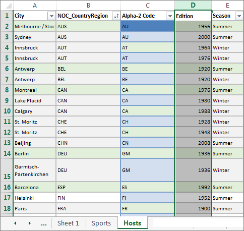
Save the workbook. Your workbook looks like the following screen.
Now that you have an Excel workbook with tables, you can create relationships between them. Creating relationships between tables lets you mash up the data from the two tables.
Create a relationship between imported data
You can immediately begin using fields in your PivotTable from the imported tables. If Excel can’t determine how to incorporate a field into the PivotTable, a relationship must be established with the existing Data Model. In the following steps, you learn how to create a relationship between data you imported from different sources.
-
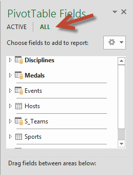
On Sheet1, at the top ofPivotTable Fields, clickAll to view the complete list of available tables, as shown in the following screen.
-
Scroll through the list to see the new tables you just added.
-
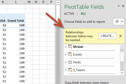
Expand Sports and select Sport to add it to the PivotTable. Notice that Excel prompts you to create a relationship, as seen in the following screen.
This notification occurs because you used fields from a table that’s not part of the underlying Data Model. One way to add a table to the Data Model is to create a relationship to a table that’s already in the Data Model. To create the relationship, one of the tables must have a column of unique, non-repeated, values. In the sample data, the Disciplines table imported from the database contains a field with sports codes, called SportID. Those same sports codes are present as a field in the Excel data we imported. Let’s create the relationship.
-
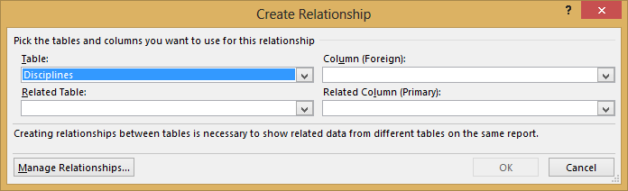
Click CREATE… in the highlighted PivotTable Fields area to open the Create Relationship dialog, as shown in the following screen.
-
In Table, choose Disciplines from the drop down list.
-
In Column (Foreign), choose SportID.
-
In Related Table, choose Sports.
-
In Related Column (Primary), choose SportID.
-
Click OK.
The PivotTable changes to reflect the new relationship. But the PivotTable doesn’t look right quite yet, because of the ordering of fields in the ROWS area. Discipline is a subcategory of a given sport, but since we arranged Discipline above Sport in the ROWS area, it’s not organized properly. The following screen shows this unwanted ordering.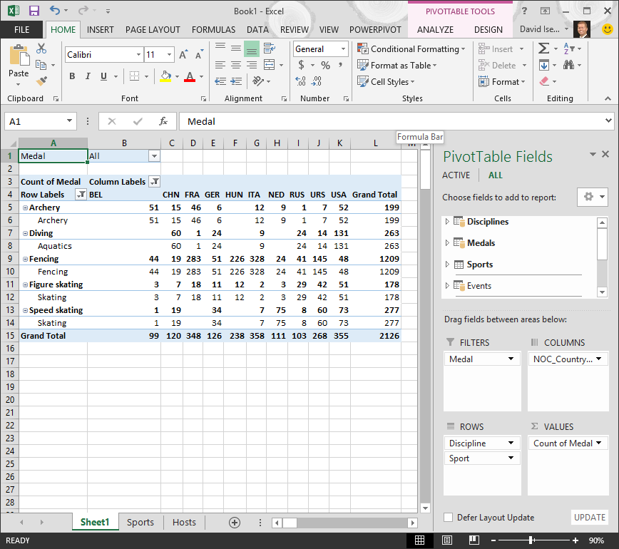
-
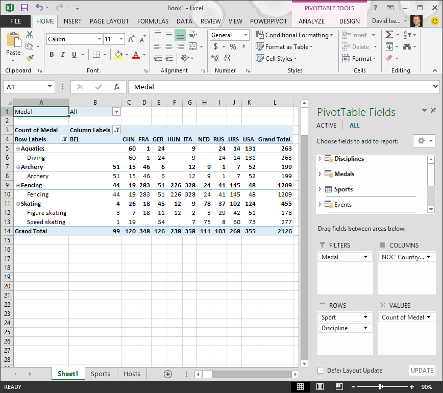
In the ROWS area, move Sport above Discipline. That’s much better, and the PivotTable displays the data how you want to see it, as shown in the following screen.
Behind the scenes, Excel is building a Data Model that can be used throughout the workbook, in any PivotTable, PivotChart, in Power Pivot, or any Power View report. Table relationships are the basis of a Data Model, and what determine navigation and calculation paths.
In the next tutorial, Extend Data Model relationships using Excel 2013, Power Pivot, and DAX, you build on what you learned here, and step through extending the Data Model using a powerful and visual Excel add-in called Power Pivot. You also learn how to calculate columns in a table, and use that calculated column so that an otherwise unrelated table can be added to your Data Model.
Checkpoint and Quiz
Review What You’ve Learned
You now have an Excel workbook that includes a PivotTable accessing data in multiple tables, several of which you imported separately. You learned to import from a database, from another Excel workbook, and from copying data and pasting it into Excel.
To make the data work together, you had to create a table relationship that Excel used to correlate the rows. You also learned that having columns in one table that correlate to data in another table is essential for creating relationships, and for looking up related rows.
You’re ready for the next tutorial in this series. Here’s a link:
Extend Data Model relationships using Excel 2013, Power Pivot, and DAX
QUIZ
Want to see how well you remember what you learned? Here’s your chance. The following quiz highlights features, capabilities, or requirements you learned about in this tutorial. At the bottom of the page, you’ll find the answers. Good luck!
Question 1: Why is it important to convert imported data into tables?
A: You don’t have to convert them into tables, because all imported data is automatically turned into tables.
B: If you convert imported data into tables, they will be excluded from the Data Model. Only when they’re excluded from the Data Model are they available in PivotTables, Power Pivot, and Power View.
C: If you convert imported data into tables, they can be included in the Data Model, and be made available to PivotTables, Power Pivot, and Power View.
D: You cannot convert imported data into tables.
Question 2: Which of the following data sources can you import into Excel, and include in the Data Model?
A: Access Databases, and many other databases as well.
B: Existing Excel files.
C: Anything you can copy and paste into Excel and format as a table, including data tables in websites, documents, or anything else that can be pasted into Excel.
D: All of the above
Question 3: In a PivotTable, what happens when you reorder fields in the four PivotTable Fields areas?
A: Nothing – you cannot reorder fields once you place them in the PivotTable Fields areas.
B: The PivotTable format is changed to reflect the layout, but underlying data is unaffected.
C: The PivotTable format is changed to reflect the layout, and all underlying data is permanently changed.
D: The underlying data is changed, resulting in new data sets.
Question 4: When creating a relationship between tables, what is required?
A: Neither table can have any column that contains unique, non-repeated values.
B: One table must not be part of the Excel workbook.
C: The columns must not be converted to tables.
D: None of the above is correct.
Quiz Answers
-
Correct answer: C
-
Correct answer: D
-
Correct answer: B
-
Correct answer: D
Notes: Data and images in this tutorial series are based on the following:
-
Olympics Dataset from Guardian News & Media Ltd.
-
Flag images from CIA Factbook (cia.gov)
-
Population data from The World Bank (worldbank.org)
-
Olympic Sport Pictograms by Thadius856 and Parutakupiu
This blog post is explaining all about how to download data from internal table to an excel file.
Requirement: On selection screen user will give the input as country name and file name in which user want to download the data to an excel file based on the given country name.
Step 1: Design Selection Screen. On selection screen declare country and file name as parameter.
SELECTION-SCREEN BEGIN OF BLOCK b1 WITH FRAME.
  PARAMETERS:p_land TYPE kna1-land1,
             p_file TYPE rlgrap-filename.
SELECTION-SCREEN END OF BLOCK b1.
Step 2: Declare structure, internal table and work area.
TYPES:
  BEGIN OF ty_kna1,
    kunnr TYPE kunnr,
    name1 TYPE name1,
    land1 TYPE land1,
    ort01 TYPE ort01,
  END OF ty_kna1.

DATA:
  it_kna1 TYPE TABLE OF ty_kna1,
  wa_kna1 TYPE ty_kna1.
Step 3: Declare variables and internal table for heading.
DATA: g_str1 TYPE string VALUE '.xls',
      g_str  TYPE string,
      g_str2 TYPE string.

DATA : BEGIN OF it_header OCCURS 0,
         line(50) TYPE c,
       END OF it_header.
Step 4: Use function module KD_GET_FILENAME_ON_F4 for F4 help for file name.
AT SELECTION-SCREEN ON VALUE-REQUEST FOR p_file.
  CALL FUNCTION 'KD_GET_FILENAME_ON_F4'
    EXPORTING
      static    = 'X'
    CHANGING
      file_name = P_file.
Step 5: Append all the heading for each field into internal table.
START-OF-SELECTION.

  it_header-line = 'Customer Number'.
  APPEND it_header.
  it_header-line = 'Customer Name'.
  APPEND it_header.
  it_header-line = 'Country'.
  APPEND it_header.
  it_header-line = 'City'.
  APPEND it_header.
Step 6: I want data in excel file so if user did not take F4 help then extension of file needs to append to file name. If user take F4 help and select excel file then no need to append extension.
IF p_file NS '.xls'.
    g_str = p_file.
    CONCATENATE g_str g_str1 INTO g_str2.
  ELSE.
    g_str2 = p_file.
  ENDIF.
Step 7: Write Select query to fetch data from database.
SELECT
    kunnr
    name1
    land1
    ort01
    FROM kna1
    INTO TABLE it_kna1
  WHERE land1 = p_land.
Step 8: Call the function module GUI_DOWNLOAD to download the data from the database into excel file.
CALL FUNCTION 'GUI_DOWNLOAD'
    EXPORTING
      filename              = g_str2
      filetype              = 'ASC'
      write_field_separator = 'X'

    TABLES
      data_tab              = it_kna1
      fieldnames            = it_header
    .
Output


Once you execute it file with name Customer excel file will be created and data will be downloaded.
If you want to download data into existing excel file Press F4 for file name.

Then Execute it, you will get data into the selected file.
Improve Article
Save Article
Like Article
Improve Article
Save Article
Like Article
Firebase is a product of Google which helps developers to build, manage, and grow their apps easily. It helps developers to build their apps faster and in a more secure way. We require No programming on the firebase side which makes it easy to use its features more efficiently. It provides services to android, iOS, web, and many more. It provides cloud storage. It uses NoSQL for the database for the storage of data.
The Firebase Realtime Database is a cloud-based NoSQL database that manages your data at the blazing speed of milliseconds. In the simplest terms, it can be considered as a big JSON file. Here we will look into the process of downloading Firebase Realtime Database in an Excel File. To do so follow the below steps:
Step 1: Go to Realtime Database Screen in your Project.
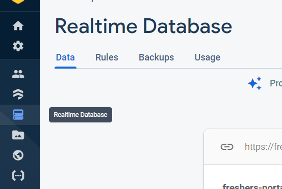
Step 2: Click on the three dots shown in the top right corner.

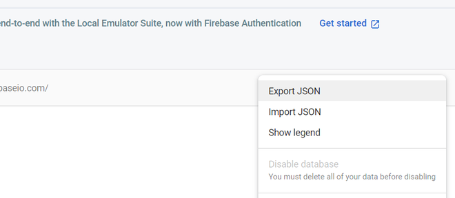
Step 3: Then Click on Export JSON file.
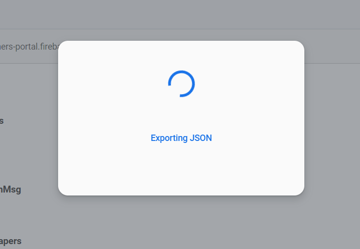
Step 4: Then you see a screen like this Exporting JSON. Then you will find that the file is downloaded in JSON format.
You can use this website to convert your JSON file into Excel format and then save your file.
Like Article
Save Article
In this tutorial, we are going to import data from a external SQL database. This exercise assumes you have a working instance of SQL Server and basics of SQL Server.
In this Excel tutorial, you will learn –
- Import SQL Data into Excel File
- How to Import Data to Excel using Wizard Dialog
- How to Import MS Access Data into Excel with Example
First we create SQL file to import in Excel. If you have already SQL exported file ready, then you can skip following two step and go to next step.
- Create a new database named EmployeesDB
- Run the following query
USE EmployeeDB
GO

CREATE TABLE [dbo].[employees](
	[employee_id] [numeric](18, 0) NOT NULL,
	[full_name] [nvarchar](75) NULL,
	[gender] [nvarchar](50) NULL,
	[department] [nvarchar](25) NULL,
	[position] [nvarchar](50) NULL,
	[salary] [numeric](18, 0) NULL,
 CONSTRAINT [PK_employees] PRIMARY KEY CLUSTERED
(
	[employee_id] ASC
)WITH (PAD_INDEX = OFF, STATISTICS_NORECOMPUTE = OFF, IGNORE_DUP_KEY = OFF, ALLOW_ROW_LOCKS = ON, ALLOW_PAGE_LOCKS = ON) ON [PRIMARY]
) ON [PRIMARY]

GO

INSERT INTO employees(employee_id,full_name,gender,department,position,salary)
VALUES
('4','Prince Jones','Male','Sales','Sales Rep',2300)
,('5','Henry Banks','Male','Sales','Sales Rep',2000)
,('6','Sharon Burrock','Female','Finance','Finance Manager',3000);

GO
How to Import Data to Excel using Wizard Dialog
- Create a new workbook in MS Excel
- Click on DATA tab

- Select from Other sources button
- Select from SQL Server as shown in the image above

- Enter the server name/IP address. For this tutorial, am connecting to localhost 127.0.0.1
- Choose the login type. Since am on a local machine and I have windows authentication enabled, I will not provide the user id and password. If you are connecting to a remote server, then you will need to provide these details.
- Click on next button
Once you are connected to the database server. A window will open, you have to enter all the details as shown in screenshot

- Select EmployeesDB from the drop down list
- Click on employees table to select it
- Click on next button.
It will open a data connection wizard to save data connection and finish the process of connecting to the employee’s data.

- You will get the following window

- Click on OK button

Download the SQL and Excel File
How to Import MS Access Data into Excel with Example
Here, we are going to import data from a simple external database powered by Microsoft Access database. We will import the products table into excel. You can download the Microsoft Access database.
- Open a new workbook
- Click on the DATA tab
- Click on from Access button as shown below

- You will get the dialogue window shown below

- Browse to the database that you downloaded and
- Click on Open button

- Click on OK button
- You will get the following data

Download the Database and Excel File
Many users are actively using Excel to generate reports for their subsequent editing. Reports are using for easy viewing of information and a complete control over data management during working with the program.
Table is the interface of the workspace of the program. A relational database structures the information in the rows and columns. Despite the fact that the standard package MS Office has a standalone application for creating and maintaining databases named Microsoft Access, users are actively using Microsoft Excel for the same purpose. After all program features allow you to: sort; format; filter; edit; organize and structure the information.
That is all that you need for working with databases. The only caveat: the Excel program is a versatile analytical tool that is more suitable for complex calculations, computations, sorting, and even for storage structured data, but in small amounts (no more than one million records in the same table, in the 2010 version).
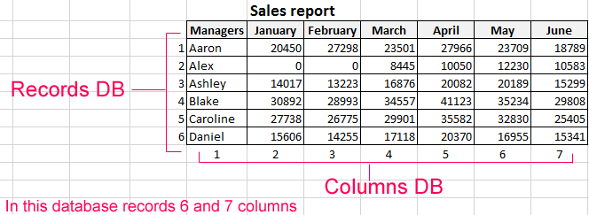
Database Structure — Excel table
Database — a data set distributed in rows and columns for easily searching, organizing and editing. How to make the database in Excel?
All information in the database is contained in the records and fields:
- Record is database (DB) line, which includes information about one object.
- Field is the column in the database that contains information of the same type about all objects.
- Records and database fields correspond to the rows and columns of a standard Microsoft Excel spreadsheet.
If you know how to do a simple table, then creating a database will not be difficult.
Creating DB in Excel: step by step instructions
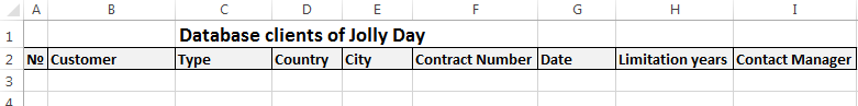
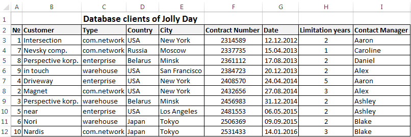
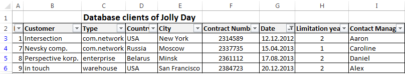
Step by step to create a database in Excel. Our challenge is to form a client database. For several years, the company has several dozens of regular customers. It is necessary to monitor the contract term, the areas of cooperation and to know contacts, data communications, etc.
How to create a customer database in Excel:
- Enter the name of the database field (column headings).
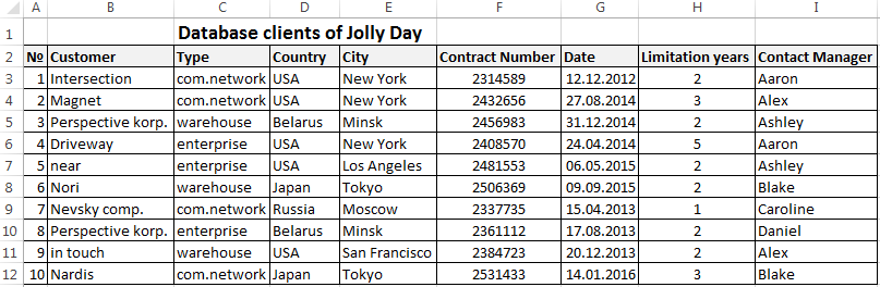
- Enter data into the database. We are keeping order in the format of the cells. If it is a numerical format so it should be the same numerical format in the entire column. Data are entered in the same way as in a simple table. If the data in a certain cell is the sum on the values of other cells, then create formula.
- To use the database turn to tools «DATA».
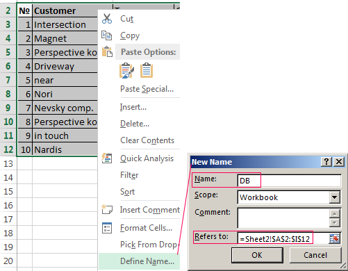
- Assign the name of the database. Select the range of data — from the first to the last cell. Right mouse button — the name of the band. We give any name. Example — DB. Check that the range was correct.
The main work of information entering into the DB is made. For easy using this information it is necessary to pick out the needful information, filter and sort the data.
How to maintain a database in Excel
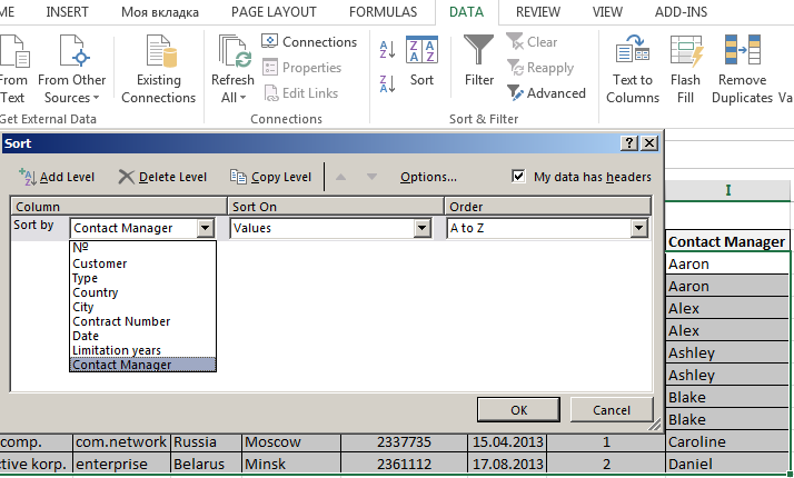
To simplify the search for data in the database, we’ll order them. Tool «Sort» is suitable for this purpose.
- Select the range you want to sort. For the purposes of our fictitious company the column «Date». Call the tool «Sort».
- Then system offers automatically expand the selected range. We agree. If we sort the data of only one column and the rest will leave in place so the information will be wrong. Then the menu will open parameters where we have to choose the options and sorting values.
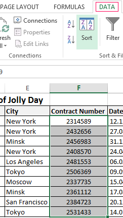
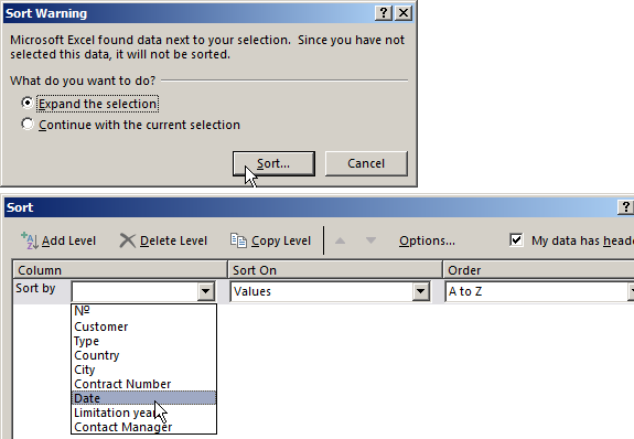
The data distributed in the table by the term of the contract.
Now, the manager sees to whom it is time to renew the contract and with which companies we continue the partnership.
Database during the company’s activity is growing to epic proportions. Finding the right information is getting harder. To find specific text or numbers you can use:
By simultaneously pressing Ctrl + F or Shift + F5. «Find and Replace» search box appears.
Filtering the data
By filtering the data the program hides all the unnecessary information that user does not need. Data is in the table, but invisible. At any time, data can be recovered.
There are 2 filters which are often used In Excel:
- AutoFilter;
- filter on the selected range.
AutoFilter offers the user the option to choose from a pre-filtering list.
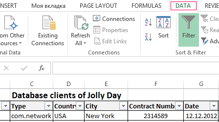
- On the «DATA» tab, click the button «Filter».
- Down arrows are appearing after clicking in the header of the table. They signal the inclusion of «AutoFilter».
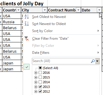
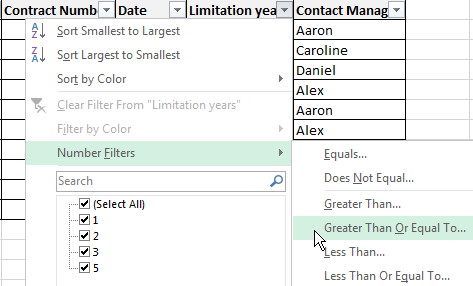
- Click on the desired column direction to select a filter setting. In the drop-down list appears all the contents of the field. If you want to hide some elements reset the birds in front of them.
- Press «OK». In the example we hide clients who have concluded contracts in the past and the current year.
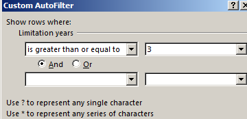
- To set a condition to filter the field type «Greater Than», «Less Than», «Equals», etc. values, select the command «Number Filters» in the filter list.
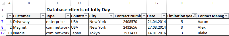
- If we want to see clients in a customer table whom we signed a contract for 3 years or more, enter the appropriate values in the AutoFilter menu.
Done!
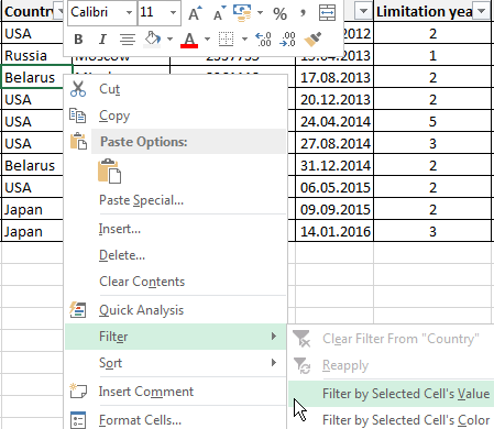
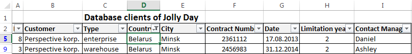
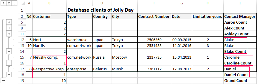
Let’s experiment with the values filtered by the selected cells. For example, we need to leave the table only with those companies that operate in Belarus.
- Select the data with information which should remain prominent in the database. In our case, we find the column country — «РБ «. We click on the cell with right-click.
- Perform a sequence command: «Filter»–«Filter by Selected Cell’s Value». Done.
Sum can be found using different parameters if the database contains financial information:
- the sum of (summarize data);
- count (count the number of cells with numerical data);
- average (arithmetic mean count);
- maximum and minimum values in the selected range;
- product (the result of multiplying the data);
- standard deviation and variance of the sample.
Using the financial information in the database:
- Then the menu will open parameters where we have to choose the options and sorting values «Contact Manager».
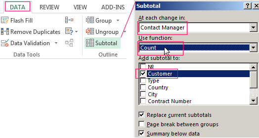
- Select the database range. Go to the tab «DATA» — «Subtotal».
- Select the calculation settings In the dialog box.
Tools on the «DATA» tab allows to segment the DB. Sort information in terms with relevance to company goals. Isolation of purchasers of goods groups help to promote the marketing of the product.
Prepared sample templates for conducting client base segment:
- Template for manager which allows monitors the result of outgoing calls to customers download.
- The simplest template. Customer in Excel free template database download.
- Example database from this article download example.
Templates can be adjusted for your needs: reduce, expand, and edit.