Down fill in excel

Использование функции мгновенного заполнения в Excel

Функция мгновенного заполнения автоматически подставляет данные, когда обнаруживает закономерность. Например, с помощью мгновенного заполнения можно разделять имена и фамилии из одного столбца или объединять их из двух разных столбцов.

Примечание: Функция мгновенного заполнения доступна только в Excel 2013 и более поздних версий.

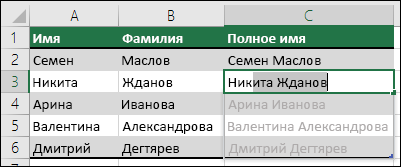
Предположим, что столбец A содержит имена, столбец B — фамилии, а вы хотите заполнить столбец C сочетаниями имен и фамилий. Если ввести полное имя в столбец C, функция мгновенного заполнения заполнит остальные ячейки соответствующим образом.

Введите полное имя в ячейке C2 и нажмите клавишу ВВОД.

Начните вводить следующее полное имя в ячейке C3. Excel определит закономерность и отобразит предварительное изображение остальной части столбца, заполненной объединенным текстом.

Для подтверждения предварительного просмотра нажмите клавишу ВВОД.

Если вариант заполнения не выводится, вероятно, эта функция не включена. Вы можете выбрать Данные > Мгновенное заполнение, чтобы применить заполнение вручную или нажать клавиши CTRL+E. Чтобы включить мгновенное заполнение, выберите Сервис > Параметры > Дополнительно > Параметры правки и установите флажок Автоматически выполнять мгновенное заполнение.

Предположим, что столбец A содержит имена, столбец B — фамилии, а вы хотите заполнить столбец C сочетаниями имен и фамилий. Если ввести полное имя в столбец C, функция мгновенного заполнения заполнит остальные ячейки соответствующим образом.

Введите полное имя в ячейке C2 и нажмите клавишу ВВОД.

Выберите Данные > Мгновенное заполнение или нажмите клавиши CTRL+E.

Excel определит закономерность в ячейке C2 и заполнит ячейки ниже.

Дополнительные сведения

Вы всегда можете задать вопрос специалисту Excel Tech Community или попросить помощи в сообществе Answers community.

Источник

Fill a formula down into adjacent cells

You can quickly copy formulas into adjacent cells by dragging the fill handle . When you fill formulas down, relative references will be put in place to ensure the formulas adjust for each row—unless you include absolute or mixed references before you fill the formula down.

Follow these steps to fill a formula and choose which options to apply:

Select the cell that has the formula you want to fill into adjacent cells.

Drag the fill handle across the cells that you want to fill.

If you don’t see the fill handle, it might be hidden. To display it again:

Click File > Options

Under Editing Options, check the Enable fill handle and cell drag-and-drop box.

To change how you want to fill the selection, click the small Auto Fill Options icon that appears after you finish dragging, and choose the option that want.

For more information about copying formulas, see Copy and paste a formula to another cell or worksheet.

Fill formulas into adjacent cells

You can use the Fill command to fill a formula into an adjacent range of cells. Simply do the following:

Select the cell with the formula and the adjacent cells you want to fill.

Click Home > Fill, and choose either Down, Right, Up, or Left.

Keyboard shortcut: You can also press Ctrl+D to fill the formula down in a column, or Ctrl+R to fill the formula to the right in a row.

Turn workbook calculation on

Formulas won’t recalculate when you fill cells if automatic workbook calculation isn’t enabled.

Here’s how you can enable it:

Click File > Options.

Under Workbook Calculation, choose Automatic.

Select the cell that has the formula you want to fill into adjacent cells.

Drag the fill handle down or to the right of the column you want to fill.

Keyboard shortcut: You can also press Ctrl+D to fill the formula down a cell in a column, or Ctrl+R to fill the formula to the right in a row.

Need more help?

You can always ask an expert in the Excel Tech Community or get support in the Answers community.

Источник

Use Excel’s Fill Down Command With Shortcut Keys

Save time and increase accuracy by copying data to other cells

Lifewire / Alison Czinkota

What to Know

• Select the source cell. Then, highlight the range to which you want to copy it and press Ctrl+D.
• Alternatively, click the fill handle in the source cell and drag it over the target cells.

This article shows how to activate the Fill Down command with a keyboard or mouse shortcut in Excel 2019, 2016, 2013, 2010, Excel Online, and Excel for Mac.

The Keyboard Method

The key combination that applies the Fill Down command is Ctrl+D.

Follow these steps to see how to use Fill Down in your own Excel spreadsheets:

Type a number into a cell.

Press and hold the Shift key.

Press and hold the Down Arrow key on the keyboard to extend the cell highlight from cell D1 to D7. Then release both keys.

Press and Ctrl+D and release.

The Mouse Method

Use your mouse to select the cell that contains the number that you want to duplicate in the cells beneath it. Then, highlight the range to which you want to copy it, and press the keyboard shortcut Ctrl+D .

Alison Czinkota / Lifewire

Use AutoFill to Duplicate the Data in a Cell

Here’s how to accomplish the same effect as the Fill Down command, but instead with the AutoFill feature:

Type a number into a cell in an Excel spreadsheet.

Click and hold the fill handle in the bottom right corner of the cell that contains the number.

Drag the fill handle downward to select the cells that you want to contain the same number.

Release the mouse and the number is copied into each of the selected cells.

The AutoFill feature also works horizontally to copy a number of adjacent cells in the same row. Just click and drag the fill handle across the cells horizontally. When you release the mouse, the number is copied into each selected cell.

Источник

Использование мгновенного заполнения в Excel

Мгновенное заполнение в Microsoft Excel – одна из функций, появившихся в последних версиях программы. Ее основное предназначение заключается в анализе сокращений, которые применяет пользователь при дублировании значения одной ячейки в другую. Один из примеров – сокращение полных имен в списке до необходимого формата, что я и рассмотрю в следующей инструкции.

Как мгновенно заполнить ячейки в Microsoft Excel

Начну с того, что Экселю необходимо обязательно знать закономерность, на основе которой он и будет осуществлять мгновенное заполнение ячеек. Например, у вас есть список месяцев с полными названиями, но вы хотите сократить их до трех букв. Значит, в ячейке напротив стоит написать «Янв» и активировать мгновенное заполнение для всей таблицы. Программа сразу поймет, как именно вы хотите сократить написание, поэтому оставит для всех остальных строк тоже только первые три буквы.

Более сложный вариант состоит как раз в использовании сокращений имени фамилии и отчества, о чем уже было сказано во вступительном абзаце. Давайте я рассмотрю его более детально, чтобы вы понимали принцип работы инструмента.

Откройте таблицу и начните с первой строки, введя такое сокращение, которое вы хотите видеть во всем остальном списке. Обратите внимание на следующий скриншот, чтобы понять, какой именно путь выбрал я в своем примере.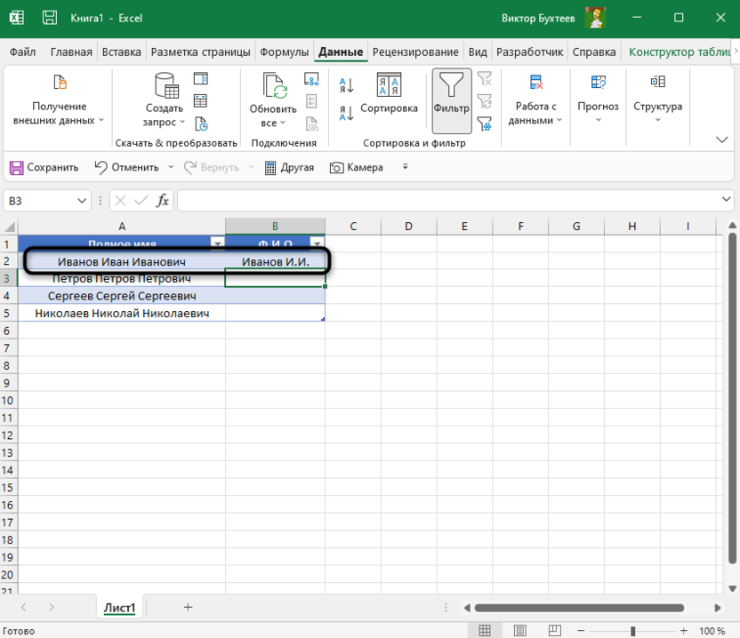

Перейдите к следующей строке и введите первую букву. Автозаполнение, включенное в Excel по умолчанию, должно предложить варианты сразу для всех ячеек таблицы. Если этого не произошло, останьтесь на первой строке с сокращением и нажмите сочетание клавиш Ctrl + E для применения опции мгновенного заполнения.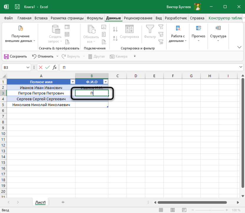

Посмотрите на результат и убедитесь в том, что у вас получилось справиться с поставленной задачей. Можете поэкспериментировать с разными сокращениями, чтобы протестировать инструмент более детально.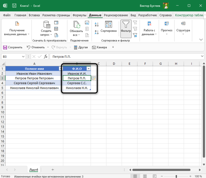

В блоке с мгновенным заполнением появится кнопка, отвечающая за открытие панели с дополнительными действиями. Так вы сможете отменить заполнение, принять предложения для ввода данных или выделить все измененные ячейки.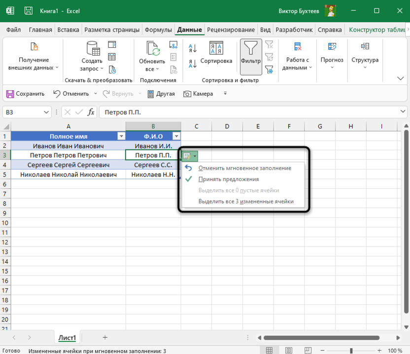

Если предложенный вариант вам не подходит, например, не работает сочетание клавиш или не появляются варианты для заполнения, можно пойти немного другим путем. Для данной опции на панели с инструментами есть своя кнопка, которая и активирует действие мгновенного заполнения.

Создайте первую строку с сокращенным вариантом и перейдите на вкладку «Данные».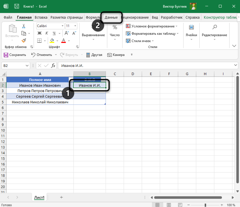

Нажмите кнопку с названием «Мгновенное заполнение».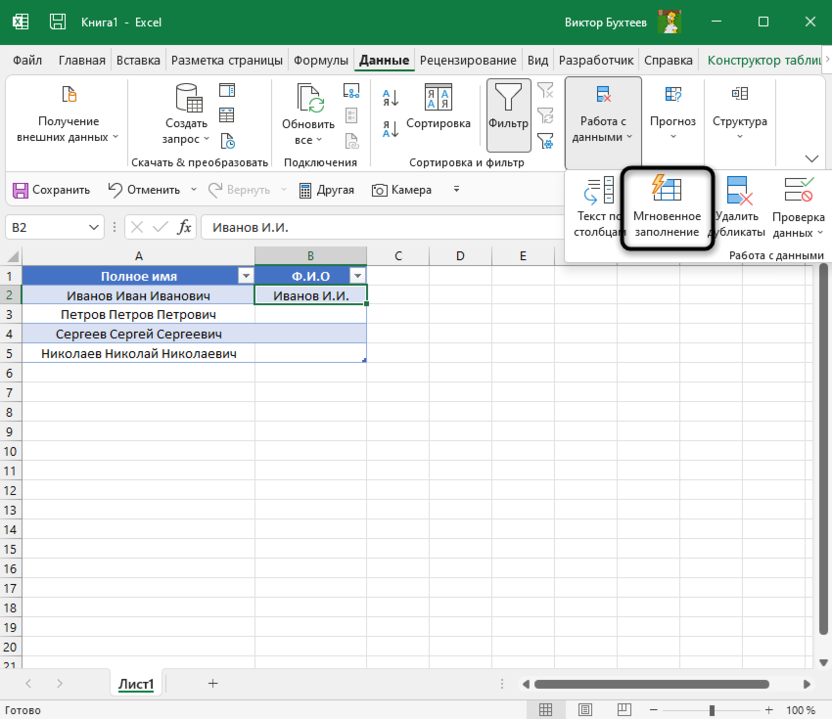

Обратите внимание на то, что инструмент вступил в силу, таблица заполнена, а вы сэкономили значительное количество времени.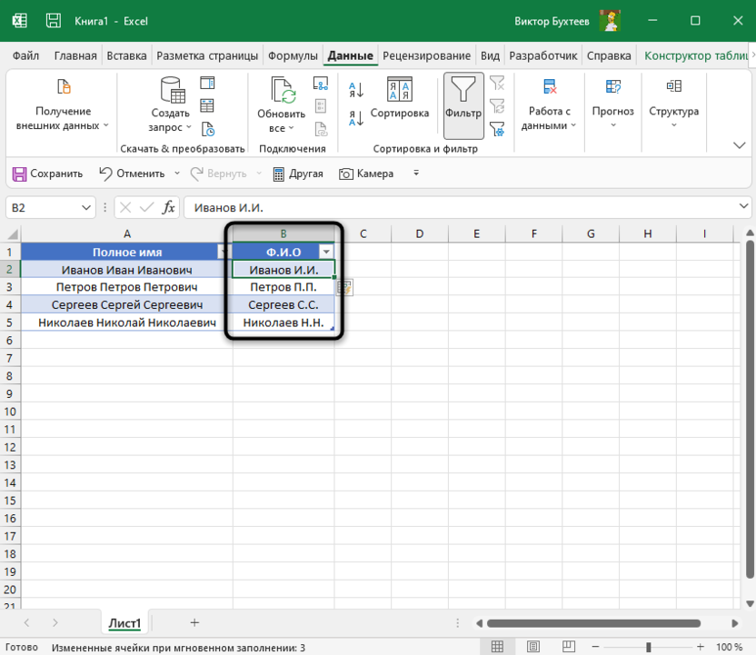

Решение некоторых проблем

В завершение быстро расскажу о том, что делать, если при редактировании ячеек не появляются варианты для мгновенного заполнения или по каким-то причинам данный инструмент не работает даже путем нажатия по соответствующей кнопке. Самая распространенная причина – отключенная функция в настройках. Ее проверка выполняется следующим образом:

Перейдите на вкладку «Файл».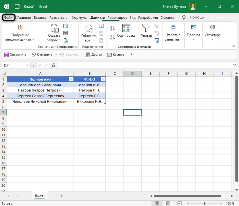

Откройте список параметров программы, щелкнув по строке с соответствующим названием.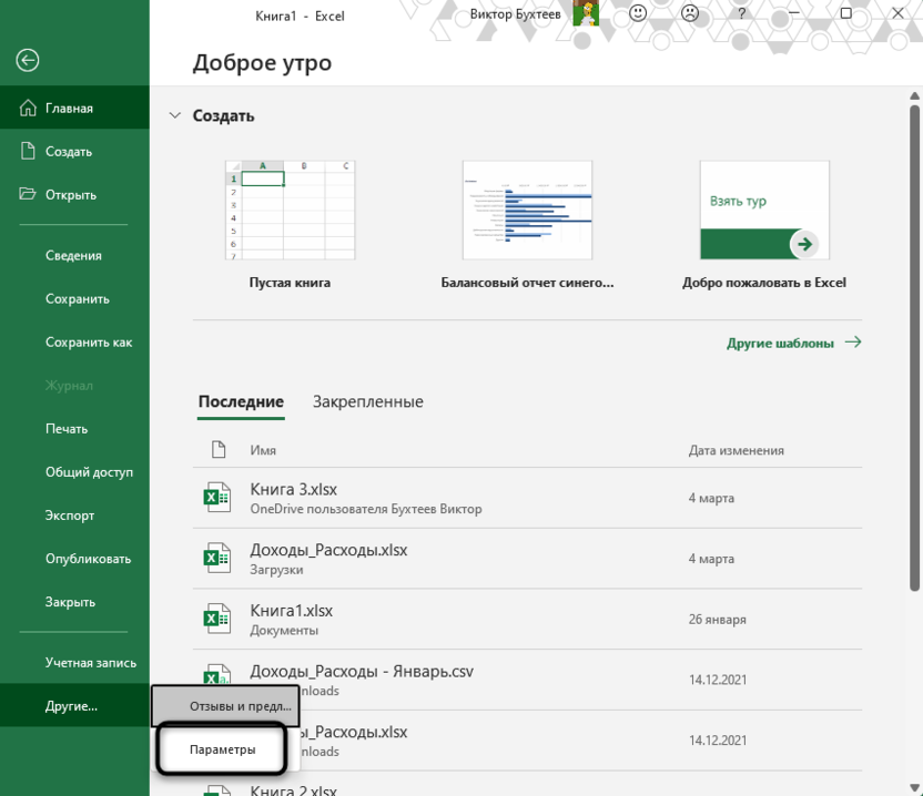

Выберите раздел «Дополнительно» и убедитесь в том, что в категории «Параметры правки» установлены галочки напротив пунктов «Автозавершение значений ячеек» и «Автоматически выполнять мгновенное заполнение».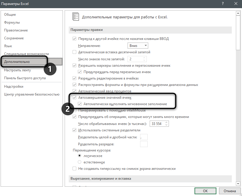

Если пункта с мгновенным заполнением вы не нашли, значит, используете старую версию Microsoft Excel и данный инструмент попросту недоступен. Установите обновление, если есть такая возможность.

Еще одна проблема – программа не может понять, как именно вы хотите использовать мгновенное заполнение. Если это так, на экране появится ошибка с соответствующим содержанием. Не закрывайте ее сразу, а прочитайте описание и сделайте все так, как пишут разработчики.

Используйте мгновенное заполнение в Microsoft Excel в своих целях, оптимизируя и значительно ускоряя рабочий процесс. Если исходные данные после сокращения вам не нужны, просто удалите их, чтобы сэкономить место в электронной таблице.

Источник

Excel Fill Down

Excel Fill Down is an option when we want to fill down or copy any data or formulas to the cells below. We can use the keyboard shortcut “CTRL + D” while copying the data and selecting the cells. Else, we can click the “Fill” button in the “Home” tab and use the option to fill it down from the list.

What is Fill Down in Excel?

In all the software, copy and paste methods are invaluable. Probably the Ctrl + C and Ctrl + V are the universal shortcut keys everyone knows. Excel is no different from other software. In Excel also, copy and paste works the same way. Apart from copying and pasting the formulas to the below cells, we can also use Excel’s option “FILL DOWN” (Ctrl + D).

Filling down the above cell value to the below cells does not necessarily require the traditional copy and paste method. Instead, we can use the option of “Fill Handle” or the Ctrl + D shortcut key.

Ctrl + D is nothing but “Fill Down.” It will fill the above cell value in Excel to the below-selected cells.

Table of contents

Excel Fill Down Shortcut

As we said, copying and pasting is the traditional method to have values in other cells. But in Excel, we can use different techniques to handle this.

Note: CTRL + D can only fill only values to below cells, not to any other cells.

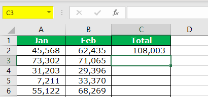
For example look at the below example data.

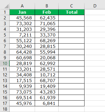
Now, we want to add the “Total” column. But, first, let us apply the simple formula in cell C2.

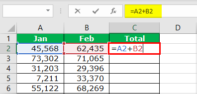
Traditionally, we copy and paste the formula to the below cells to have a formula applied for all the below cells. But, we place a cursor on the right bottom end of the formula cell.

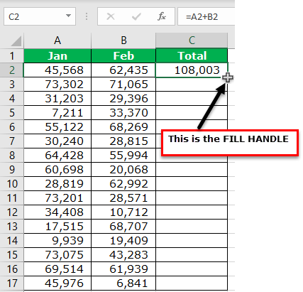
We need to double-click on the “FILL HANDLE.” As a result, it will fill the current cell formula to all the below cells.

How cool is it to fill the formula rather than copy and paste?

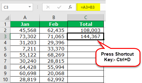
Instead of using “FILL HANDLE” and “Copy-Paste,” we can use the Excel “Fill Down” shortcut in excel Shortcut In Excel An Excel shortcut is a technique of performing a manual task in a quicker way. read more Ctrl + D to fill down values from the above cell.

Place a cursor on the C3 cell.

Now, press the shortcut key Ctrl + D. We will have the relative formula from the above cell.

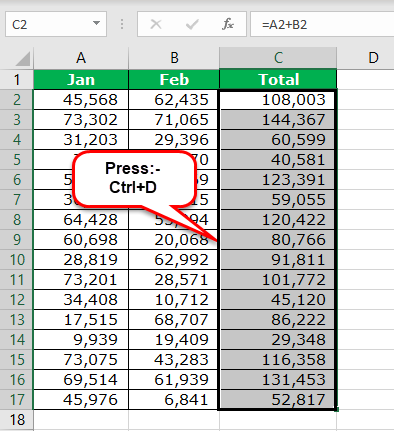
In order to fill all the cells. First, select the formula cell until the last cell of the data.

Now, press Ctrl + D. It will fill the formula for all the selected cells.

Fill Blank Cells with Above Cell Value

It is one of the toughest challenges I have faced early on. Before telling you the challenge, let me show you the data first.

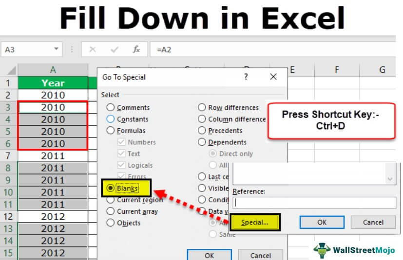
In the above data, I was asked by my manager to fill in Excel the year to the remaining cells until we found the other year, i.e., I have to fill 2010 year from A3 cell to A6 cell.

It is the sample of the data, but there was a huge amount of data it needed me to fill. Therefore, I spent one extra hour than my usual time to complete the task.

However, I later learned the technique to fill these void cells with the above cell value. Therefore, follow the below steps to apply the same logic.

Step 1: We must first select all the cells in the data range.

Step 2: Now press the F5 key. As a result, we may see a “Go To” window.

Step 3: Now, we need to press on “Special.”

Step 4: In the below “Go To Special” window, select “Blanks.”

It will select all the blank cells in the chosen area.

Step 5: Now, do not move the cursor to select any cells. Rather, press equal and give a link to the above cell.

Step 6: After giving a link to the above cell, do not simply press the “Enter” key. Using different logic here will help; instead of pressing the “Enter” key, press ENTER key by holding the CTRL-key.

Consequently, it will fill the values of all the selected cells.

Since the first incident, I have not extended my shift for these silly reasons.

I have moved on from CTRL + C to CTRL + D in Excel

I recently realized the benefit of CTRL + D while working with large Excel files. I deal with 5 lakhs to 10 lakhs of rows of data every day in my daily job. Often, I require to fetch the data from one worksheet to another. I have to apply various formulas to fetch the data from different workbooks.

When I copied and pasted the formula to the cells, it usually took more than 10 minutes to complete the formula. Can you imagine what I was doing all these 10 minutes?

I hit my computer and almost begged my Excel to finish the process fast. I was frustrated that I had to wait for more than 10 minutes every time for every formula.

Later, I started using the Excel “FILL DOWN,” CTRL + D to fill the formula below cells. Then, I realized that it only took 2 minutes, not more than that.

So, I have moved on from Ctrl + C to Ctrl + D in Excel.

Things to Remember While Fill Down in Excel

• The Ctrl + D shortcut can only fill down. It neither fills to the right nor left.
• The Ctrl + Enter shortcut can fill the values to all the selected cells in the worksheet.
• The “FILL HANDLE” also fills down instead of dragging the formula.
• We must use the Ctrl + D shortcut to fill down and Ctrl + R to fill right.

Recommended Articles

This article has been a guide to Fill Down in Excel. We discussed filling blank cells with the above cell value using Excel fill-down shortcuts, practical examples, and a downloadable Excel template. You may learn more about Excel from the following articles: –

Источник