Dollar sign in excel

We’ve noticed some of you searching for help using “$” – a dollar sign. In Excel, a dollar sign can denote a currency format, but it has another common use: indicating absolute cell references in formulas. Let’s consider both uses of the dollar sign in Excel.

Dollar signs denoting currency

If you want to display numbers as monetary values, you must format those numbers as currency. To do this, you apply either the Currency or Accounting number format to the cells that you want to format. The number formatting options are available on the Home tab, in the Number group.

What’s the difference between the two number formats? There are two main differences:

1. The Currency format displays the currency symbol adjacent to the number, whereas the Accounting format displays the symbol at the edge of the cell, regardless of the length of the number.
2. The Accounting format displays zeros as dashes and negative numbers in parentheses, whereas the Currency format displays zeros as zeros and denotes negative numbers by using a minus sign (-). For more information, see the article Display numbers as currency.

Dollar signs indicating absolute references

You probably know that a formula can refer to cells. That’s one reason Excel formulas are so powerful — the results can change based on changes made in other cells. When a formula refers to a cell, it uses a cell reference. In the “A1” reference style (the default), there are three kinds of cell references: absolute, relative, and mixed.

Absolute cell references

When a formula contains an absolute reference, no matter which cell the formula occupies the cell reference does not change: if you copy or move the formula, it refers to the same cell as it did in its original location. In an absolute reference, each part of the reference (the letter that refers to the row and the number that refers to the column) is preceded by a “$” – for example, $A$1 is an absolute reference to cell A1. Wherever the formula is copied or moved, it always refers to cell A1.

Relative cell references

In contrast, a relative reference changes if the formula is copied or moved to a different cell (i.e., a cell other than where the formula was originally entered). The row and column portions of a relative reference are not preceded by a “$” –  for example, A1 is a relative reference to cell A1. If moved or copied, the reference changes by the same number of rows and coulmns as it was moved. So, if you move a formula with the relative reference A1 one cell down and one cell to the right, the reference changes to B2.

Mixed cell references

A mixed reference uses a dollar sign either in front of the row letter or in front of the column number, but not both – for example, A$1 is a mixed reference in which the row adjusts, but the column does not. So if you move a formula containing that reference one cell down and one cell to the right, it becomes B$1.

Which kind of cell reference should you use?

The kind of cell reference you use depends on what you are doing, but usually you want to use relative references. Excel uses relative references by default, which makes it easy to fill formulas down and across: the references automatically update, which is what you want, most of the time.

One case where you might want to use an absolute reference is when using the VLOOKUP function. Though the value you’re wanting to look up might change (for example, as you fill the VLOOKUP formula down a column), the actual location of the lookup table doesn’t change or adjust as you fill the column down.

But now that you know the differences between these kinds of cell references, you can make the decision for yourself, based on how you want your formulas to behave. Do you have some use-cases to share with the community? Share them by leaving a comment!

— Steven Thomas

If you have worked with Excel formulas, I am sure you have noticed that sometimes there is a $ symbol as a part of the cell references.

If you’re wondering what does the $ sign means in Excel formulas/functions, this article is the right place.

One of the things that make Excel such a powerful tool is the ability to refer to cells/ranges and use these in formulas.

And when you copy these formulas, these cell references can adjust automatically (or should I say automatically).

Below is an example where I copy the cell C2 (which has a formula) and paste it in C3.

You can see that the formula adjusts the references when I copy and paste it. While in the formula in cell C2 refers to A2 and B2, the one in C3 refers to A3 and B3.

This is called relative reference where the references adjust based on the cell in which it has been applied.

But what if you don’t want some cells to adjust the reference?

What if you want to copy the formula, but don’t want the cell reference to change?

…. introducing the $ sign.

When you use a $ sign before the cell reference (such as $C$2), you’re telling Excel to keep referring to cell C3 even when you copy and paste the formula.

Now you can use the dollar ($) sign in three different ways, which means that there are three types of references on Excel.

Shortcut to add $ Sign to Cell References

There are two ways you can add the $ sign to a cell reference in Excel.

You can either do it manually (i.e., go into the edit mode in a cell by double-clicking on it or using F2, placing the cursor where you want the $ sign and then typing it manually).

Or you can use the keyboard shortcut

 F4 

To use this shortcut, simply place the cursor on the cell reference where you want to add the dollar sign and press is once. You will notice that it will change the reference by adding/removing the $ sign (based on what’s the original reference).

For example, suppose you have the reference C2 in a cell. Here is how the F4 shortcut would work:

• Press F4 one time – C2 will change to $C$2
• Press F4 two times – C2 will change to C$2
• Press F4 three times – C2 will change to $C2
• Press F4 four times – C2 will change back to C2

Types of References in Excel

There are three types of references in Excel:

• Relative references
• Absolute references
• Mixed references

In relative references, you don’t use a dollar ($) sign in the references at all.

In mixed references, you use the dollar sign ($) only once (such as $C3 or C$3)

In absolute reference, you use the dollar sign in twice in a reference (such as $C$3).

Let me quickly explain each of these with a simple example.

Relative reference

Relative reference is where you don’t use a dollar ($) sign at all.

And when you copy a cell that has a relative reference, it will change and adjust based on the cell where you copy it.

Below is the same example again, where the references adjust as soon as we copy and paste the cell that has the formula.

Absolute reference

In absolute references, you have the $ sign before the row number and the column alphabet (example $C$3)

When you use this in formulas, it will not change the reference

when you copy and paste the cell. This could be useful when you have some value that needs to remain constant (such as time period or interest rates, etc.)

Below is an example where I have a value in cell D2 which needs to remain constant (and not change when we copy-paste the formulas).

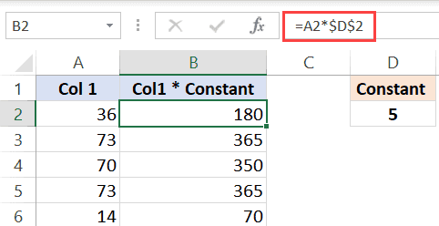
By using $D$2, we make sure that it doesn’t change when we copy-paste the cell with the formula.

Note that this example has both, relative cell reference (without the $ sign) and an absolute cell reference (with two $ signs).

Note: If you’re wondering why not simply hard code the value instead of using the absolute cell reference (the one with two dollar signs). While you can use the value itself, in the future, if you have to change the value in formulas, you will have to manually do it. Instead, you can simply change the value in C3, and all the formulas would automatically update.

Mixed reference

These are a little more complicated than the rest two.

In mixed cell references, you will have only one dollar sign (for example – $C3 or C$3)

When you add a dollar sign in front of the column alphabet (C in this example), it locks the column only. This means that if you copy-paste the formula that uses $C3, the column would not change, but the row can change.

And when you add a dollar sign in front of the row number (3 in this example), it locks the column only. This means that if you copy-paste the formula that uses C$3, the row would not change, but the column can change.

Here is a good article that goes in-depth about the mixed cell references in Excel.

Summary

A dollar sign means that the part of the cell reference before which it has been used is anchored or fixed.

Below is a quick summary of what $ means in Excel formulas:

1. $A$1 – always refers to column A and row 1
2. $A1 – Column A is fixed and will not change, but the row is allowed to change as the formula is copied
3. A$1 – Row 1 is fixed and will not change, but the column is allowed to change as the formula is copied.
4. $A$1:$A$100 – always refers to the range A1:A100

I hope this article helps you understand what the $ sign means in Excel and how to use it.

Other Excel tutorials you may find useful:

• How to Remove Dollar Sign in Excel
• How to Remove Dashes (-) in Excel?
• How to Lock Cells in Excel [Mac, Windows]
• How to Apply Accounting Number Format in Excel
• What does Pound/Hash Symbol (####) Mean in Excel?
• What Does the Exclamation Point Mean in Excel?

When some Excel users see Dollar signs in an Excel formula it generally brings about a fair amount of confusion.  Many Excel users starting out will often skip this learning but honestly if you want to progress as an Excel analyst or use Excel to create amazing tools you must understand what the Dollars signs are for and how to use them, it’s simple and I will show you everything you need to know in this post.

What are the dollar signs?

If you see a formula that looks something like:

=B3 * $A$1

This is an example of using Dollar signs in Excel formula.

Why use the Dollar signs?

The Dollar signs are used for indicating Absolute References.  Now that statement might not be too helpful but to understand what I mean there are two ways you can reference a cell location, either using a Relative Reference (no Dollar signs) or some form of Absolute Reference (Dollar signs involved).

Relative Reference

Relative Referencing is the default option with Excel formulas.  If you have created any kind of basic Excel formula then the chances are you used this method, you probably were not aware you were using it but trust me if you referenced a cell, for example A1, in your formula and you had no Dollar signs then you used a Relative Reference.

A Relative Reference describes how Excel is able to understand the underlying meaning of the formula and automatically translate it across other cells when you drag or copy the formula to other cells.

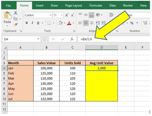
Take the below example where the aim is to calculate the Average Unit Value in Column D.  To calculate Average Unit Value the Sales Value in Column B must be Divided by the Units Sold in Column C.

You could enter a straight mathematical equation in cell D4, i.e. =100,000/1,000 but that will be no good to drag down to the next cell D5, you would have to type out that formula for every cell in Column D.

The right way is to use Relative Referencing to tell Excel is should Divide the Cell 2 Columns to the left by the Cell 1 Column to the left, so for cell D4 that means the formula is =B4/C4:

By using the Relative Reference system it will allow you to drag the formula down and apply it to February, March, April and so on without having to enter a new formula every time.

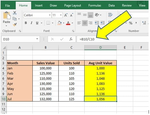
As you can see in the below image dragging the formula that you created in cell D4 down to cell D10 Excel auto-calculates the correct Average Unit Value for every month, when you look at the formula in cell D10 it has automatically changed to =B10/C10.  Remember this is still saying take the Cell 2 Columns to the left and Divide it by the Cell 1 Column to the left:

As mentioned previously Relative References are commonly used and most of you will be using them without even realizing what they are.

However, there are times when you need to fix the cell location in some way and this is where Absolute Referencing comes in and our Dollar signs.

Absolute Reference

Using Absolute References is where you start using the Dollar signs in your Excel formula.  The Dollar signs tell Excel that you want to fix a specific part of a cell location and stop it from changing when you drag or copy the formula to other cells.  There are three ways cell location can be fixed.

What are the three ways that I can use Dollar Signs in my Excel formula?

You can create a fixed point on:

1. The Column position
2. The Row position
3. Both column and row positions which is the same as fixing a specific cell.

To set the fixed-point add a Dollar sign ($) in front of the part of the cell reference that you want to fix, for example:

= $A1  …. This means Column A is the fixed-point as the Dollar sign is before the Column letter A.  If you copy or drag this formula anywhere else on the worksheet it will always reference back to Column A.  The Row will change depending on where the formula is copied.

= A$1  …. This means Row 1 is the fixed-point as the Dollar sign is before the Row number 1.  If you copy or drag this formula anywhere else on the worksheet it will always reference back to Row 1.  The Column will change depending on where the formula is copied.

= $A$1 …. This means Cell A1 is the fixed-point as there is a Dollar sign before the Column letter and the Row Number.  No matter where you copy or drag this formula on the Excel worksheet it will always refer to Cell A1.

An Example using relative references

Referring back to the previous Example imagine if you now have a Sales Commission of 10% that your boss wants included in the table.  You could use a formula that multiplies the Sales Value by the value of 10% but what if your boss then tells you the Commission rate was wrong or needs to be changed?  It would mean you need to change all the formulas in every cell again and that is not very efficient.

Instead you can use Absolute Referencing to set a Commission % Cell and then always refer to that Cell in your formula.  By doing this if you want to change the Commission to a hefty 20% and see how it affects the numbers you only need to change one value in the Commission % Cell and all the totals will recalculate:

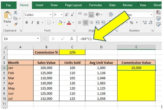
In the image above the Commission % Cell is in Cell C10 and it has been set to 10%.  In the Commission Value column of the table (Column E) the first formula is entered to Cell E4 which is =B4*C1.

Remember that to Excel the underlying meaning of this formula is take the Cell 3 columns to the left(B4) and multiply it by the Cell 2 Columns to the left and 3 Rows up (C1).  If you leave this formula as it is watch what happens when it is dragged down to E10:

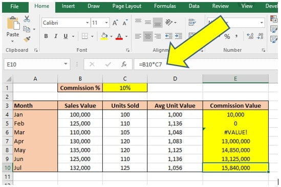
As you can see the formula starts fine in Cell E4 but as soon as you drag the formula down the other months it goes horribly wrong.  To see the problem you only need to look in Cell E10 which shows the formula to be = B10 * C7.  This is clearly not what was intended as while B10 is the correct Sales Value to use C7 is the Units Sold in May and not the Commission percentage.

What did we do wrong?

We forgot to set the Absolute Reference.

Excel is doing its job, remember Excel thinks it should be multiplying the Cell 3 Columns to the left by the Cell 2 Columns to the left and 3 Rows up…if you do a quick zoom around the table that is working so it’s not Excels fault, the fault is with us.

What you need to do is change the underlying meaning to Excel by saying Multiply the cell 3 columns to the left by the cell C1 and always the cell C1 as that is the Commission %.  Change the formula:

You can see from the above image the formula in Cell E4 now reads = B4 * $C$1.

Referring back remember that a Dollar sign before the Column location and before the Cell location is the same as making a specific Cell a fixed-point.  By including the Dollar sign before the Column letter C and before the Row number 1 the Cell C1 becomes a fixed-point and the underlying meaning is changed to multiply the Cell 3 Columns to the left by the value in C1, drag that version down the table and see the results:

The formula has now worked as planned.  A quick check again in Cell E10 shows that the formula is multiplying B10 (the cell 3 columns to the left) by C1, perfect!

Any other tips for using Dollar Signs in Excel formula?

To use Absolute References in Excel formula you can manually type the Dollar signs around the cell location or you can simply toggle the 3 Absolute Reference options using the shortcut key of F4.

To use the Shortcut key make sure the cursor is directly to the left of your cell reference, i.e. if you want to add absolute references to = 50 * A1 then make sure the cursor is flashing to the left of A, then hit F4.  Hit F4 once and it will turn it into a fixed cell location, hit F4 again and it will change to just a fixed row location and finally hit F4 a third time if you want just the column to be fixed.

Summary

I hope this helps some of you out there understand the use of Dollar signs in Excel formula.  As an Excel beginner this can be a topic many skip over but going forward in your Excel learning and development it becomes a crucial technique to understand.

As usual if you have some comments please leave them below or get in touch with me on Twitter.

Keep Excelling,

If you are looking to improve your Excel knowledge and impress the boss, or perhaps build some amazing tools that you can use for your own business then I highly recommend the following Excel book available from Amazon, click on the image to pick up your copy today:

You can also use Excel’s formatting tools to automatically represent numbers as currency. To do so, highlight a cell, group of cells, row or column and click the “Home” tab in Excel’s ribbon menu. Click the “$” sign in the “Number” group of icons in the menu to put the cells into Accounting format.

What is the fastest way to add dollar signs in Excel?

As long as the cursor is in the reference, or immediately before or after it, you can use the function key F4, to toggle through the options above (in the order shown). That’s it, pressing F4 once adds both dollars, twice fixes the row, three times fixes the column, four times removes the dollars again.

How do you add the dollar sign?

To create the dollar sign symbol using a U.S. keyboard, hold down the Shift and press 4 at the top of the keyboard.

What is a $1 in Excel?

A$1. Allows the column reference to change, but not the row reference. $A$1. Allows neither the column nor the row reference to change. There is a shortcut for placing absolute cell references in your formulas!

What is F4 in Excel?

F4: Repeat your last action. If you have a cell reference or range selected when you hit F4, Excel cycles through available references. Shift+F4: Repeat the last find action.

What does F5 key do in Excel?

F5. Displays the Go To dialog box. For example, to select cell C15, in the Reference box, type C15, and click OK. Note: you can also select named ranges, or click Special to quickly select all cells with formulas, comments, conditional formatting, constants, data validation, etc.

What is the difference between a $1 and $A1 in Excel?

A reference to $A$1in a formula would remain unchanged when you copy it. $A1 would adjust the row number when copied but would still point to column A. And A$1 would keep the row number the same while adjusting the column reference.

Where do I find symbols in Excel?

Using the Symbol menu

• To open the menu, click the Insert tab in the Ribbon, then click Symbol:
• You’ll see the Symbol menu:
• From here, you can scroll through hundreds of symbols.

What does #value mean in Excel?

#VALUE is Excel’s way of saying, “There’s something wrong with the way your formula is typed. Or, there’s something wrong with the cells you are referencing.” The error is very general, and it can be hard to find the exact cause of it.

What does Alt R do in Excel?

In Microsoft Excel, pressing Alt + R opens the Review tab in the Ribbon. After using this shortcut, you can press an additional key to select a Review tab option.

What is Ctrl F3 in Excel?

You can bring up the Name Manager in Excel by pressing Ctrl + F3. This lists the names used in your current workbook, and you can also define new names, edit existing names or delete names from the Name Manager.

What does F11 do in Excel?

F11 Creates a chart of the data in the current range in a separate Chart sheet. Shift+F11 inserts a new worksheet. Alt+F11 opens the Microsoft Visual Basic For Applications Editor, in which you can create a macro by using Visual Basic for Applications (VBA).

What does F2 do on Excel?

Everybody (well, almost everybody) knows that pressing the F2 key in Excel activates the “editing” mode for the active cell – the cursor goes into the cell so that you can change the contents and the various cell references in that formula turn different colours.

What is B $5 Excel?

B$1:B$5 when copied across to the right by one column; A$1:A$5 (no change) when copied down by one row.

What does Alt F9 do in Excel?

Ctrl+Alt+F9: Calculates all worksheets in all open workbooks, regardless of whether they have changed since the last calculation.

Why is the dollar sign not showing in Excel?

Left-click and drag over the range of cells in which you want to display the dollar sign. If you want the sign to appear in an entire column, click the column letter at the top. If you want to select an entire row, click the row number on the left side. For a single cell, simply click the cell.

How do I paste a range name in Excel?

Pasting a Range Name to Another Location

1. First, select the cell where you wish the range name to be pasted.
2. In the Ribbon, select Formulas > Defined Names > Use in Formula > Paste Names…
3. Select the name you want to paste, then click OK.
4. Press the Enter key on the keyboard or click the check mark in the formula bar.

Where is AutoFill in Excel?

Select cell A1 and cell A2 and drag the fill handle down. The fill handle is the little green box at the lower right of a selected cell or selected range of cells. Note: AutoFill automatically fills in the numbers based on the pattern of the first two numbers.

What are symbols in Excel?

Symbols used in Excel Formula

Symbol	Name
()	Parentheses
*	Asterisk
,	Comma
&	Ampersand

How do I insert a symbol in Excel without the formula?

All formulas in spreadsheet programs, like Microsoft Excel, OpenOffice Calc, and Google Sheets start with an equal sign (=). To display an equal sign, but not have it start a formula, you must “escape” the cell by entering a single quote (‘) at the beginning.

How do I add special characters to a cell in Excel?

Select the desired symbol on the Symbols tab; or click the Special Characters tab and select the desired character. Click Insert to insert the symbol or character. Click Close when you’re done adding symbols and special characters. Press Enter to complete the cell entry.

Home / Excel Basics / How to Add Dollar Sign in Excel

In Excel, users add the $ dollar sign at the beginning of the value, representing the value as monetary value. you can also convert the standard numeric values into monetary values by adding the $ sign in front of them.

There are multiple ways to add the $ Dollar sign in Excel, like manually adding the $ sign in the cells or changing the cells’ format to currency or accounting format.

This tutorial will show you how to add the $ Dollar sign in the cells in multiple ways.

Add the Dollar Sign by typing the $ Sign

1. First, go to the cell and double-click in the cell or press “Fn +F2” keys to put the cell in edit mode.
2. After that, move the cursor to the left side in front of the value and press the “Shift + $” keys together, and the $ sign will get added in front of the value.
   
3. Once the $ sign got added into the cell, use the Format Painter to copy and paste the formatting into the rest of the cells to auto-add the $ sign into them.
   

Add Dollar Sign using Concatenate Function

You can use the CONCATENATE function to add the $ sign with the values in the cell by following the below steps:

1. First, go to the cell and write the “Concatenate” formula.
2. In the formula, as shown in the below image, after the open parentheses, enter the dollar sign “$” and enter a comma, then select the cell reference (B2) where you have the value, and then close the parentheses and press enter.
   
3. After that, hover the mouse on the below right corner of the cell, and double-right-click to copy the formula to the rest of the cells.
   
4. Copy the cells range with the formula and paste special to the cells where you want to have $ sign with values and then convert them to numeric values as shown below in the image.
   

Add Dollar Sign using Text Function

You can also use the text function to add the $ sign in the cells by following the below steps:

1. First, go to the blank cell and write the “TEXT” formula.
2. In the formula, as shown in the below image, after the open parentheses, select the cell reference (B2) where you have the value with which you want to add the $ sign and enter a comma and then write the “$00” as format text value and close the parentheses and press enter.
   
3. After that, hover the mouse on the below right corner of the cell, and double-right-click to copy the formula to the rest of the cells.
4. Copy the cells range with the formula and paste special to the cells where you want to have $ sign with values and then convert them to numeric values as shown below in the image.
   

Add Dollar Sign by Converting the Cells Formatting to Currency or Accounting Format

1. First, select the cells range and go to the “Home” tab.
2. After that, click on the “Format” drop-down arrow under the “Number” group and choose the “Currency” or “Accounting” option from the menu.
3. Once you choose any of the two formats, it will add a $ sign in the cells in the front of the values.

The only difference between the currency and accounting format is that in currency formatting, it places the $ sign at the beginning of the value. In accounting format, it places the $ sign in the extreme left or, you can say, at the beginning of the cell.

Shortcut to Apply Currency Format to Add Dollar Sign

You can convert the cell formatting to currency formatting using the keyboard shortcut to Currency Format:

Ctrl + Shift + $