
Содержание
- What Do the Symbols (&,$,<, etc.) Mean in Formulas? – Excel & Google Sheets
- Equal Sign (=)
- Standard Operators
- Order of Operations and Adding Parentheses
- Colon (:) to Specify a Range of Cells
- Dollar Symbol ($) in an Absolute Reference
- Exclamation Point (!) to Indicate a Sheet Name
- Square Brackets [ ] to Refer to External Workbooks
- Comma (,)
- Refer to Multiple Ranges
- Separate Arguments in a Function
- Curly Brackets in Array Formulas
- Other Important Symbols
- Symbols in Formulas in Google Sheets
- What does $ (dollar sign) mean in Excel Formulas?
- What does $ mean in Excel formulas?
- Shortcut to add $ Sign to Cell References
- Types of References in Excel
- Relative reference
- Absolute reference
- Mixed reference
- Summary
- Mean, median and mode in Excel
- How to calculate mean in Excel
- How to find median in Excel
- How to calculate mode in Excel
- Mean vs. median: which is better?
What Do the Symbols (&,$,<, etc.) Mean in Formulas? – Excel & Google Sheets
This tutorial explains what different symbols mean in formulas in Excel and Google Sheets.
Excel is essentially used for keeping track of data and using calculations to manipulate this data. All calculations in Excel are done by means of formulas, and all formulas are made up of different symbols or operators, depending on what function the formula is performing.
Equal Sign (=)
The most commonly used symbol in Excel is the equal (=) sign. Every single formula or function used has to start with equals to let Excel know that a formula is being used. If you wish to reference a cell in a formula, it has to have an equal sign before the cell address. Otherwise, Excel just shows the cell address as standard text.
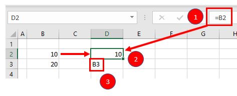
In the above example, if you type (1) =B2 in cell D2, it returns a value of (2) 10. However, typing only (3) B3 into cell D3 just shows “B3” in the cell, and there is no reference to the value 20.
Standard Operators
The next most common symbols in Excel are the standard operators as used on a calculator: plus (+), minus (–), multiply (*) and divide (/). Note that the multiplication sign is not the standard multiplication sign (x) but is depicted by an asterisk (*) while the division sign is not the standard division sign (÷) but is depicted by the forward slash (/).
An example of a formula using addition and multiplication is shown below:
Order of Operations and Adding Parentheses
In the formula shown above, B2*B3 is calculated first, as in standard mathematics. The order of operations is always multiplication before addition. However, you can adjust the order of operations by adding parentheses (round brackets) to the formula; any calculations between these parentheses would then be done first before the multiplication. Parentheses, therefore, are another example of symbols used in Excel.
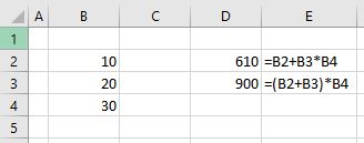
In the example shown above, the first formula returns a value of 610 while the second formula (using parentheses) returns 900.
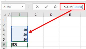
Parentheses are also used with all Excel functions. For example, to sum B3, B4, and B5 together, you can use the SUM Function where the range B3:B5 is contained within parentheses.
Colon (:) to Specify a Range of Cells
In the formula used above, the parentheses contain the cell range which the SUM Function needs to add together. This cell range is expressed with a colon (:) where the first cell reference (B3) is the cell address of the first cell included in the range of cells to add together, while the second cell reference (B5) is the cell address of the last cell included in the range.
Dollar Symbol ($) in an Absolute Reference
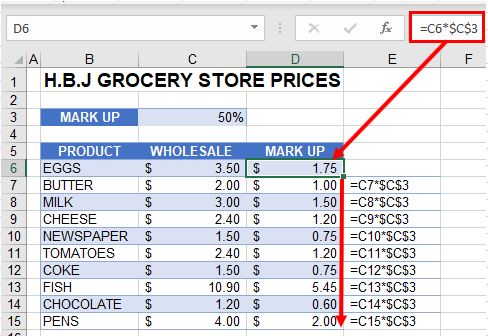
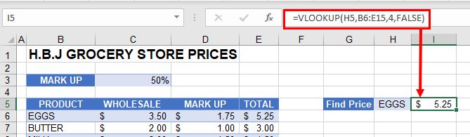
A particular useful and common symbol used in Excel is the dollar sign within a formula. Note that this does not indicate currency; rather, it’s used to “fix” a cell address in place in order that a single cell can be used repetitively in multiple formulas by copying formulas between cells.
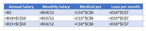
By adding a dollar sign ($) in front of the column header (C) and the row header (3), when copying the formula down to Rows 7–15 in the example below, the first part of the formula (e.g., C6) changes according to the row it is copied down to while the second part of the formula ($C$3) stays static always enabling the formula to refer to the value stored in cell C3.
See: Cell References and Absolute Cell Reference Shortcut for more information on absolute references.
Exclamation Point (!) to Indicate a Sheet Name
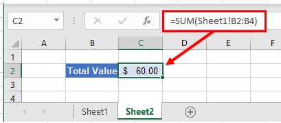
The exclamation point (!) is critical if you want to create a formula in a sheet and include a reference to a different sheet.
Square Brackets [ ] to Refer to External Workbooks
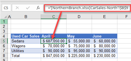
Excel uses square brackets to show references to linked workbooks. The name of the external workbook is enclosed in square brackets, while the sheet name in that workbook appears after the brackets with an exclamation point at the end.
Comma (,)
The comma has two uses in Excel.
Refer to Multiple Ranges
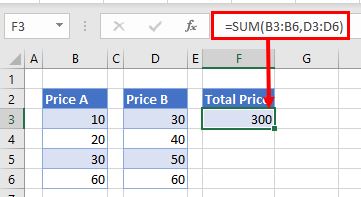
If you wish to use multiple ranges in a function (e.g., the SUM Function), you can use a comma to separate the ranges.
Separate Arguments in a Function
Alternatively, some built in Excel functions have multiple arguments which are usually separated with commas. (These can also be semicolons, depending on the function syntax.)
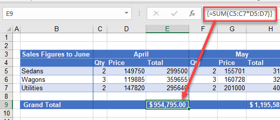
Curly Brackets in Array Formulas
Curly brackets are used in array formulas. An array formula is created by pressing the CTRL + SHIFT + ENTER keys together when entering a formula.
Other Important Symbols
| Symbol | Description | Example |
|---|---|---|
| % | Percentage | =B2% |
| ^ | Exponential operator | =B2^B3 |
| & | Concatenation | =B2&B3 |
| > | Greater than | =B2>B3 |
| = | Greater than or equal to | =B2>=B3 |
| Not equal to | =B2<>B3 |
Symbols in Formulas in Google Sheets
The symbols used in Google Sheets are identical to those used in Excel.
Источник
What does $ (dollar sign) mean in Excel Formulas?
If you have worked with Excel formulas, I am sure you have noticed that sometimes there is a $ symbol as a part of the cell references.
If you’re wondering what does the $ sign means in Excel formulas/functions, this article is the right place.
Table of Contents
What does $ mean in Excel formulas?
One of the things that make Excel such a powerful tool is the ability to refer to cells/ranges and use these in formulas.
And when you copy these formulas, these cell references can adjust automatically (or should I say automatically).
Below is an example where I copy the cell C2 (which has a formula) and paste it in C3.
You can see that the formula adjusts the references when I copy and paste it. While in the formula in cell C2 refers to A2 and B2, the one in C3 refers to A3 and B3.
This is called relative reference where the references adjust based on the cell in which it has been applied.
But what if you don’t want some cells to adjust the reference?
What if you want to copy the formula, but don’t want the cell reference to change?
…. introducing the $ sign.
When you use a $ sign before the cell reference (such as $C$2), you’re telling Excel to keep referring to cell C3 even when you copy and paste the formula.
Now you can use the dollar ($) sign in three different ways, which means that there are three types of references on Excel.
Shortcut to add $ Sign to Cell References
There are two ways you can add the $ sign to a cell reference in Excel.
You can either do it manually (i.e., go into the edit mode in a cell by double-clicking on it or using F2, placing the cursor where you want the $ sign and then typing it manually).
Or you can use the keyboard shortcut
To use this shortcut, simply place the cursor on the cell reference where you want to add the dollar sign and press is once. You will notice that it will change the reference by adding/removing the $ sign (based on what’s the original reference).
For example, suppose you have the reference C2 in a cell. Here is how the F4 shortcut would work:
- Press F4 one time – C2 will change to $C$2
- Press F4 two times – C2 will change to C$2
- Press F4 three times – C2 will change to $C2
- Press F4 four times – C2 will change back to C2
Types of References in Excel
There are three types of references in Excel:
- Relative references
- Absolute references
- Mixed references
In relative references, you don’t use a dollar ($) sign in the references at all.
In mixed references, you use the dollar sign ($) only once (such as $C3 or C$3)
In absolute reference, you use the dollar sign in twice in a reference (such as $C$3).
Let me quickly explain each of these with a simple example.
Relative reference
Relative reference is where you don’t use a dollar ($) sign at all.
And when you copy a cell that has a relative reference, it will change and adjust based on the cell where you copy it.
Below is the same example again, where the references adjust as soon as we copy and paste the cell that has the formula.
Absolute reference
In absolute references, you have the $ sign before the row number and the column alphabet (example $C$3)
When you use this in formulas, it will not change the reference
when you copy and paste the cell. This could be useful when you have some value that needs to remain constant (such as time period or interest rates, etc.)
Below is an example where I have a value in cell D2 which needs to remain constant (and not change when we copy-paste the formulas).
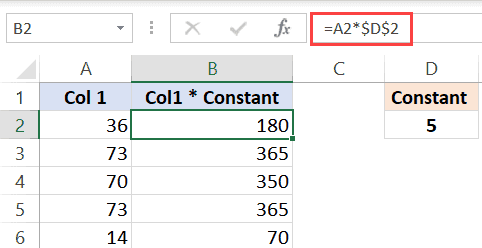
By using $D$2, we make sure that it doesn’t change when we copy-paste the cell with the formula.
Note that this example has both, relative cell reference (without the $ sign) and an absolute cell reference (with two $ signs).
Mixed reference
These are a little more complicated than the rest two.
In mixed cell references, you will have only one dollar sign (for example – $C3 or C$3)
When you add a dollar sign in front of the column alphabet (C in this example), it locks the column only. This means that if you copy-paste the formula that uses $C3, the column would not change, but the row can change.
And when you add a dollar sign in front of the row number (3 in this example), it locks the column only. This means that if you copy-paste the formula that uses C$3, the row would not change, but the column can change.
Here is a good article that goes in-depth about the mixed cell references in Excel.
Summary
A dollar sign means that the part of the cell reference before which it has been used is anchored or fixed.
Below is a quick summary of what $ means in Excel formulas:
- $A$1 – always refers to column A and row 1
- $A1 – Column A is fixed and will not change, but the row is allowed to change as the formula is copied
- A$1 – Row 1 is fixed and will not change, but the column is allowed to change as the formula is copied.
- $A$1:$A$100 – always refers to the range A1:A100
I hope this article helps you understand what the $ sign means in Excel and how to use it.
Other Excel tutorials you may find useful:
Источник
 by Svetlana Cheusheva, updated on March 20, 2023
When analyzing numerical data, you may often be looking for some way to get the «typical» value. For this purpose, you can use the so-called measures of central tendency that represent a single value identifying the central position within a data set or, more technically, the middle or center in a statistical distribution. Sometimes, they are also classified as summary statistics.
The three main measures of central tendency are Mean, Median and Mode. They all are valid measures of central location, but each gives a different indication of a typical value, and under different circumstances some measures are more appropriate to use than others.
How to calculate mean in Excel
Arithmetic mean, also referred to as average, is probably the measure you are most familiar with. The mean is calculated by adding up a group of numbers and then dividing the sum by the count of those numbers.
For example, to calculate the mean of numbers <1, 2, 2, 3, 4, 6>, you add them up, and then divide the sum by 6, which yields 3: (1+2+2+3+4+6)/6=3.
In Microsoft Excel, the mean can be calculated by using one of the following functions:
- AVERAGE- returns an average of numbers.
- AVERAGEA — returns an average of cells with any data (numbers, Boolean and text values).
- AVERAGEIF — finds an average of numbers based on a single criterion.
- AVERAGEIFS — finds an average of numbers based on multiple criteria.
For the in-depth tutorials, please follow the above links. To get a conceptual idea of how these functions work, consider the following example.
In a sales report (please see the screenshot below), supposing you want to get the average of values in cells C2:C8. For this, use this simple formula:
To get the average of only «Banana» sales, use an AVERAGEIF formula:
=AVERAGEIF(A2:A8, «Banana», C2:C8)
To calculate the mean based on 2 conditions, say, the average of «Banana» sales with the status «Delivered», use AVERAGEIFS:
=AVERAGEIFS(C2:C8,A2:A8, «Banana», B2:B8, «Delivered»)
You can also enter your conditions in separate cells, and reference those cells in your formulas, like this: 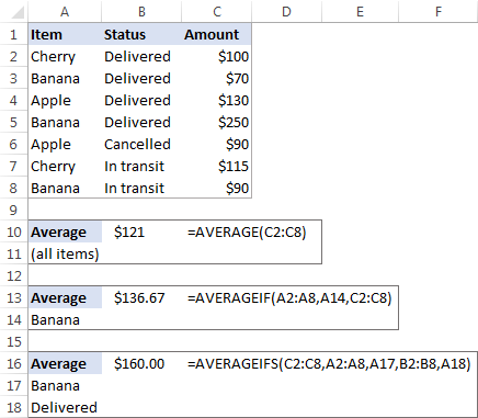
Median is the middle value in a group of numbers, which are arranged in ascending or descending order, i.e. half the numbers are greater than the median and half the numbers are less than the median. For example, the median of the data set <1, 2, 2, 3, 4, 6, 9>is 3. 
This works fine when there are an odd number of values in the group. But what if you have an even number of values? In this case, the median is the arithmetic mean (average) of the two middle values. For example, the median of <1, 2, 2, 3, 4, 6>is 2.5. To calculate it, you take the 3rd and 4th values in the data set and average them to get a median of 2.5. 
In Microsoft Excel, a median is calculated by using the MEDIAN function. For example, to get the median of all amounts in our sales report, use this formula:
To make the example more illustrative, I’ve sorted the numbers in column C in ascending order (though it is not actually required for the Excel Median formula to work): 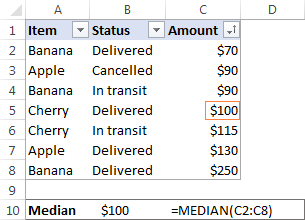
In contrast to average, Microsoft Excel does not provide any special function to calculate median with one or more conditions. However, you can «emulate» the functionality of MEDIANIF and MEDIANIFS by using a combination of two or more functions like shown in these examples:
How to calculate mode in Excel
Mode is the most frequently occurring value in the dataset. While the mean and median require some calculations, a mode value can be found simply by counting the number of times each value occurs.
For example, the mode of the set of values <1, 2, 2, 3, 4, 6>is 2. In Microsoft Excel, you can calculate a mode by using the function of the same name, the MODE function. For our sample data set, the formula goes as follows:
=MODE(C2:C8) 
In situations when there are two or more modes in your data set, the Excel MODE function will return the lowest mode.
Generally, there is no «best» measure of central tendency. Which measure to use mostly depends on the type of data you are working with as well as your understanding of the «typical value» you are attempting to estimate.
For a symmetrical distribution (in which values occur at regular frequencies), the mean, median and mode are the same. For a skewed distribution (where there are a small number of extremely high or low values), the three measures of central tendency may be different.
Since the mean is greatly affected by skewed data and outliers (non-typical values that are significantly different from the rest of the data), median is the preferred measure of central tendency for an asymmetrical distribution.
For instance, it is generally accepted that the median is better than the mean for calculating a typical salary. Why? The best way to understand this would be from an example. Please have a look at a few sample salaries for common jobs:
- Electrician — $20/hour
- Nurse — $26/hour
- Police officer — $47/hour
- Sales manager — $54/hour
- Manufacturing engineer — $63/hour
Now, let’s calculate the average (mean): add up the above numbers and divide by 5: (20+26+47+54+63)/5=42. So, the average wage is $42/hour. The median wage is $47/hour, and it is the police officer who earns it (1/2 wages are lower, and 1/2 are higher). Well, in this particular case the mean and median give similar numbers.
But let’s see what happens if we extend the list of wages by including a celebrity who earns, say, about $30 million/year, which is roughly $14,500/hour. Now, the average wage becomes $2,451.67/hour, a wage that no one earns! By contrast, the median is not significantly changed by this one outlier, it is $50.50/hour. 
Agree, the median gives a better idea of what people typically earn because it is not so strongly affected by abnormal salaries.
This is how you calculate mean, median and mode in Excel. I thank you for reading and hope to see you on our blog next week!
Источник
How to Find Mean in Excel (Table of Content)
- Introduction to Mean in Excel
- Example of Mean in Excel
Introduction to Mean in Excel
The average function is used to calculate the Arithmetic Mean of the given input. It is used to do sum of all arguments and divide it by the count of arguments where the half set of the number will be smaller than the mean, and the remaining set will be greater than the mean. It will return the arithmetic mean of the number based on provided input. It is an in-built Statistical function. A user can give 255 input arguments in the function.
As an example, suppose there is 4 number 5,10,15,20 if a user wants to calculate the mean of the numbers then it will return 12.5 as the result of =AVERAGE (5, 10, 15, 20).
The formula of Mean: It is used to return the mean of the provided number where a half set of the number will be smaller than the number, and the remaining set will be greater than the mean.
The argument of the Function:
- number1: It is a mandatory argument in which functions will take to calculate the mean.
- [number2]: It is an optional argument in the function.
Examples on How to Find Mean in Excel
Here are some examples of how to find mean in excel with the steps and the calculation
You can download this How to Find Mean Excel Template here – How to Find Mean Excel Template
Example #1 – How to Calculate the Basic Mean in Excel
Let’s assume there is a user who wants to perform the calculation for all numbers in Excel. Let’s see how we can do this with the average function.
Step 1: Open MS Excel from the start menu >> Go to Sheet1, where the user has kept the data.
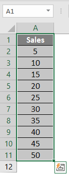
Step 2: Now create headers for Mean where we will calculate the mean of the numbers.
![]()
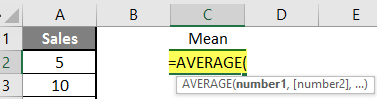
Step 3: Now calculate the mean of the given number by average function>> use the equal sign to calculate >> Write in cell C2 and use average>> “=AVERAGE (“
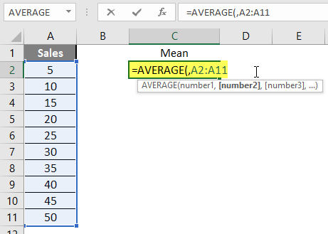
Step 3: Now, it will ask for a number1, which is given in column A >> there are 2 methods to provide input either a user can give one by one or just give the range of data >> select data set from A2 to A11 >> write in cell C2 and use average>> “=AVERAGE (A2: A11) “
Step 4: Now press the enter key >> Mean will be calculated.
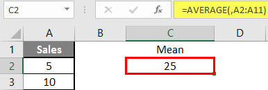
Summary of Example 1: As the user wants to perform the mean calculation for all numbers in MS Excel. Easley everything calculated in the above excel example, and the Mean is 27.5 for sales.
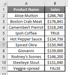
Example #2 – How to Calculate Mean if Text Value Exists in the Data Set
Let’s calculate the Mean if there is some text value in the Excel data set. Let’s assume a user wants to perform the calculation for some sales data set in Excel. But there is some text value also there. So, he wants to use count for all, either its text or number. Let’s see how we can do this with the AVERAGE function. Because in the normal AVERAGE function, it will exclude the text value count.
Step 1: Open MS Excel from the start menu >> Go to Sheet2, where the user has kept the data.
Step 2: Now create headers for Mean where we will calculate the mean of the numbers.
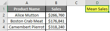
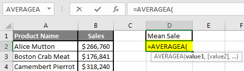
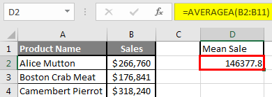
Step 3: Now calculate the mean of the given number by average function>> use the equal sign to calculate >> Write in cell D2 and use AVERAGEA>> “=AVERAGEA (“
Step 4: Now, it will ask for a number1, which is given in column B >> there is two open to provide input either a user can give one by one or just give the range of data >> select data set from B2 to B11 >> write in D2 Cell and use average>> “=AVERAGEA (D2: D11) “
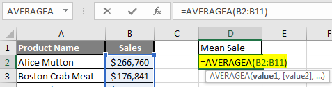
Step 5: Now click on the enter button >> Mean will be calculated.
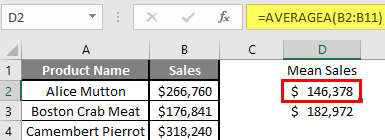
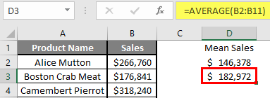
Step 6: Just to compare the AVERAGEA and AVERAGE, in normal average, it will exclude the count for text value so mean will high than the AVERAGE MEAN.
Summary of Example 2: As the user wants to perform the mean calculation for all number in MS Excel. Easley, everything calculated in the above excel example and the Mean is $146377.80 for sales.
Example #3 – How to Calculate Mean for Different Set of Data
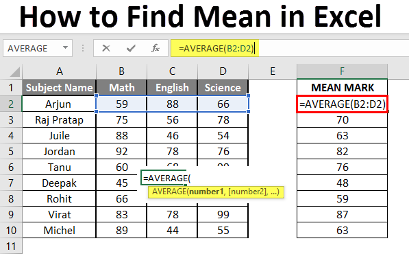
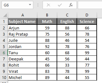
Let’s assume a user wants to perform the calculation for some student’s mark data set in MS Excel. There are ten student marks for Math, English, and Science out of 100. Let’s see How to Find Mean in Excel with the AVERAGE function.
Step 1: Open the MS Excel from the start menu >> Go to Sheet3, where the user kept the data.
Step 2: Now create headers for Mean where we will calculate the mean of the numbers.
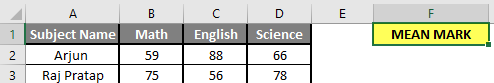
Step 3: Now calculate the mean of the given number by average function>> use the equal sign to calculate >> Write in F2 Cell and use AVERAGE >> “=AVERAGE (“
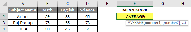
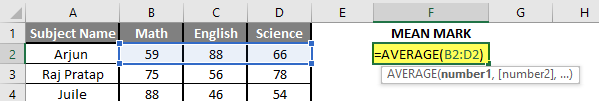
Step 3: Now, it will ask for number1 which is given in B, C, and D column >> there is two open to provide input either a user can give one by one or just give the range of data >> Select data set from B2 to D2 >> Write in F2 Cell and use average >> “=AVERAGE (B2: D2) “
Step 4: Now click on the enter button >> Mean will be calculated.
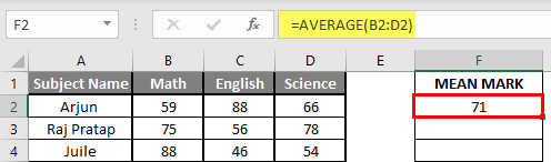
Step 5: Now click on the F2 cell and drag and apply to another cell in the F column.
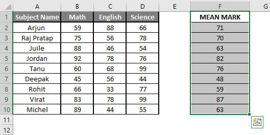
Summary of Example 3: As the user wants to perform the mean calculation for all number in MS Excel. Easley, everything calculated in the above excel example and the Mean is available in the F column.
Things to Remember About How to Find Mean in Excel
- Microsoft Excel’s AVERAGE function used to calculate the Arithmetic Mean of the given input. A user can give 255 input arguments in the function.
- Half the set of a number will be smaller than the mean, and the remaining set will be greater than the mean.
- If a user calculating the normal average, it will exclude the count for a text value, so AVERAGE Mean will bigger than the AVERAGE MEAN.
- Arguments can be number, name, range or cell references that should contain a number.
- If a user wants to calculate the mean with some condition, then use AVERAGEIF or AVERAGEIFS.
Recommended Articles
This is a guide to How to Find Mean in Excel. Here we discuss How to Find Mean along with examples and a downloadable excel template. You may also look at the following articles to learn more –
- FIND Function in Excel
- Excel Find
- Excel Average Formula
- Excel AVERAGE Function
-

1
Open Microsoft Excel. Click or double-click the Excel app icon, which resembles a green «X» on a green-and-white background.
- If you already have an Excel document that contains your data, double-click the document to open it in Excel 2007, then skip ahead to finding the mean.
-
2
Select a cell for your first data point. Click once the cell in which you want to enter your first number.
- Be sure to select a cell in a column that you want to use for the rest of your points.
Advertisement
-
3
Enter a number. Type in one of your data points’ numbers.
-
4
Press ↵ Enter. Doing so will both enter the number into your selected cell and move your cursor down to the next cell in the column.
-
5
Enter each of the rest of your data points. Type in a data point, press Enter, and repeat until you’ve entered all of your data points in the same column. This will make it easier to calculate the mean and the standard deviation of the list.


Advertisement
-
1
Click an empty cell. Doing so places your cursor in the cell.
-
2
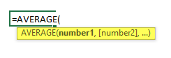
Enter the «mean» formula. Type =AVERAGE( ) into the cell.[1]
-
3
Place your cursor in between the parentheses. You can press the left arrow key once to do this, or you can click in between the two parentheses in the text box at the top of the document.
-
4
Add your data range. You can input a range of data cells by typing the name of the first cell in the list of data, typing a colon, and typing in the last cell name in the column. For example, if your list of numbers goes from cell A1 through cell A11, you would type in A1:A11 in between the parentheses.
- Your completed formula should look something like this: =AVERAGE(A1:A11)
- If you want to calculate the mean of a few numbers (not a whole range), you can type each number’s cell name between the parentheses and separate the names with commas. For example, to find the mean of A1, A3, and A10, you would type in =AVERAGE(A1,A3,A10).
-
5
Press ↵ Enter. Doing so will run your formula, causing the mean of your selected values to display in your currently selected cell.


Advertisement
-
1
Click an empty cell. Doing so places your cursor in the cell.
-
2
Enter the «standard deviation» formula. Type =STDEV( ) into the cell.[2]
-
3
Place your cursor in between the parentheses. You can press the left arrow key once to do this, or you can click in between the two parentheses in the text box at the top of the document.
-
4
Add your data range. You can input a range of data cells by typing the name of the first cell in the list of data, typing a colon, and typing in the last cell name in the column. For example, if your list of numbers goes from cell A1 through cell A11, you would type in A1:A11 in between the parentheses.
- Your completed formula should look something like this: =STDEV(A1:A11)
- If you want to calculate the standard deviation of a few numbers (not a whole range), you can type each number’s cell name between the parentheses and separate the names with commas. For example, to find the standard deviation of A1, A3, and A10, you would type in =STDEV(A1,A3,A10).
-
5
Press ↵ Enter. Doing so will run your formula, causing the standard deviation value for your selected values to display in your currently selected cell.


Advertisement
Add New Question
-
Question
If the data set has 0 in it, should we include that when calculating mean? What about if the data set has blank cells; will these be considered zeroes when calculating mean?

If there is a 0 among your data set, it should be included when calculating the mean. Blank cells are not considered as zeroes in Excel, even if they are not excluded from the data range.
Ask a Question
200 characters left
Include your email address to get a message when this question is answered.
Submit
Advertisement
-
Changing a value in one of your data range’s cells will cause any connected formulas to refresh with an updated solution.
-
You can actually use the above instructions in any more-recent version of Excel (e.g., Excel 2016) as well.
Thanks for submitting a tip for review!
Advertisement
-
Double-check your list of data points before attempting to calculate mean or standard deviation.
Advertisement
About This Article
Thanks to all authors for creating a page that has been read 895,394 times.
Is this article up to date?
Microsoft Excel 2010 is designed to store numerical inputs and permit calculation on those numbers, making it an ideal program if you need to perform any numerical analysis such as computing the mean, median, mode and range for a set of numbers. Each of these four mathematical terms describes a slightly different way of looking at a set of numbers and Excel has a built-in function to determine each of them except for the range, which will require that you create a simple formula to find.
-
Open a new Microsoft Excel 2010 spreadsheet by double-clicking the Excel icon.
-
Click on cell A1 and enter the first number in the set of numbers that you are investigating. Press «Enter» and the program will automatically select cell A2 for you. Enter the second number into cell A2 and continue until you have entered the entire set of numbers into column A.
-
Click on cell B1. Enter the following formula, without quotes, to find the arithmetic mean of your set of numbers: «=AVERAGE(A:A)». Press «Enter» to complete the formula and the mean of your numbers will appear in the cell.
-
Select cell B2. Enter the following formula, without quotes, into the cell: «=MEDIAN(A:A)». Press «Enter» and the median of your set of numbers will appear in the cell.
-
Click cell B3. Enter the following formula, without quotes, into the cell: «=MODE.MULT(A:A)». Press «Enter» and the cell will display mode of the data set.
-
Select cell B4. Enter the following formula, without quotes, into the cell: «=MAX(A:A)-MIN(A:A)». Press «Enter» and the cell will display the range for your set of data.
There are many functions in order to find the average in Excel (although it does not matter what kind of value it is: numerical, textual, percentage or other). And each of them has its own peculiarities and advantages. After all, certain conditions can be put in this task.
For example, the average in Excel is counting using statistical functions. You can also manually enter your own formula. Consider the various options.
How to find the arithmetic mean?
It is necessary to add all the numbers in the set and divide the sum by the number in order to find the arithmetic mean. For example, the student’s marks in computer science: 3, 4, 3, 5, 5. The average rating is 4 for a quarter. We found the arithmetic mean using the formula: =(3 + 4 + 3 + 5 + 5) / 5.
How can you quickly do this with Excel functions? Take for example a number of random numbers in a row:

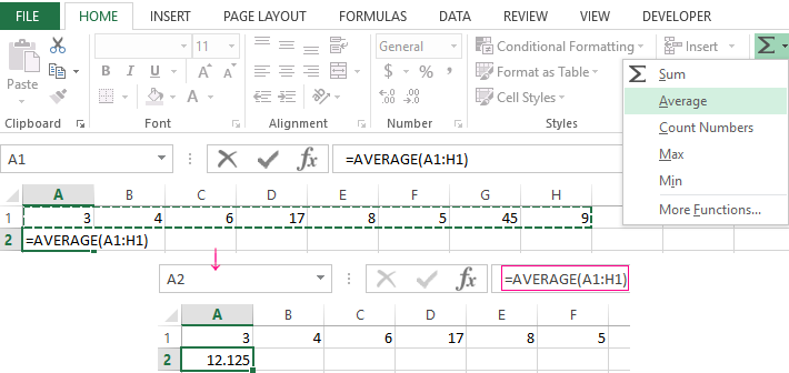
- We put the cursor in cell A2 (under a set of numbers). In the menu – «HOME»-«Editing»-«AutoSum»-«Average» button. A formula appears after clicking in the active cell. Select the range: A1: H1 and press ENTER.
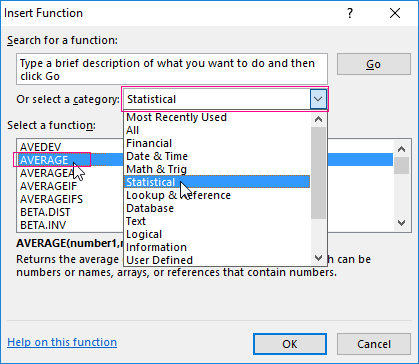
- The second method is based on the same principle of finding the arithmetic mean. But we will call the function AVERAGE differently. Using the function wizard (use fx button or key combination SHIFT + F3).
- The third way to call the AVERAGE function from the panel: «FORMULAS»-«More Function»-«Statistical»-«AVERAGE».
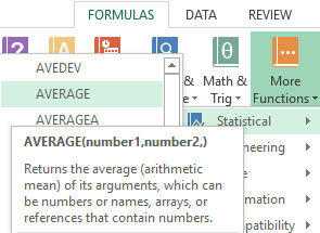
Or you can make cell to be active and just manually enter the formula: =AVERAGE(A1:A8).
Now let’s see what the AVERAGE function be able to:
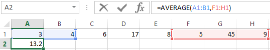
Let us find the arithmetic mean of the first two and three last numbers. Formula: =AVERAGE(A1:B1,F1:H1).
Average value by condition
A numerical criterion or a textual criterion can be the condition for finding the arithmetic mean. We will use the function: = AVERAGEIF().
Find the arithmetic mean for numbers that are greater or equal to 10.
Function:
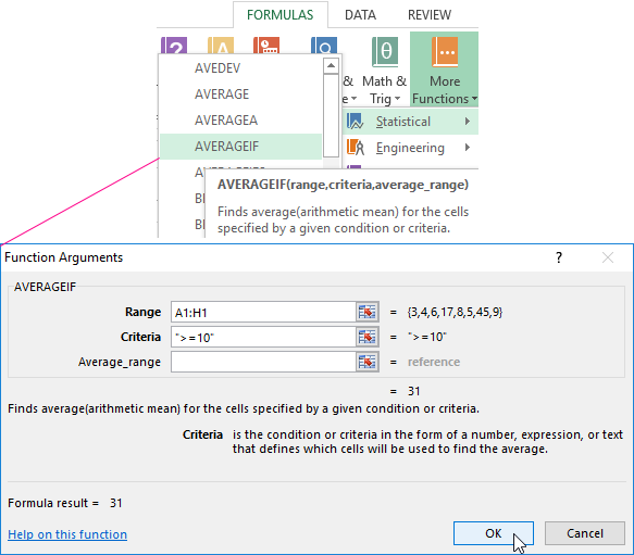
The result of using the function «AVERAGEIF» by the condition «>=10» is next:
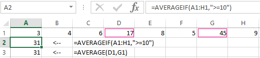
The third argument «Averaging Range» is omitted. Firstly, it is not necessary. Secondly, the range analyzed by the program contains ONLY numeric values. In the cells specified in the first argument, the search will be performed according to the condition specified in the second argument.
Attention! You can specify the search criteria in the cell. And in the formula make a reference to it.
Let’s find the average value of numbers by the text criterion. For example, the average sales of goods «Tables».
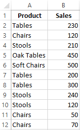
The function will look like this:
Range is a column with the names of goods. Search criteria is a link to a cell with the word «Tables» (you can insert the word «Tables» instead of the A7 link). The averaging range is the cells from which data will be taken to calculate the arithmetic mean.
We get the following value as a result of calculating using the function:
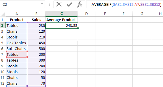
Attention! It is mandatory to point the averaging range for the text criterion (condition).
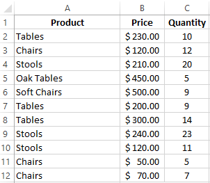
How to calculate the weighted average price in Excel?
How to calculate the average percentage in Excel? For this purpose, the SUMPRODUCTS and SUM functions are suitable. Table for an example:
How did we know the weighted average price?
Formula:
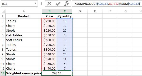
Using the formula =SUMPRODUCT() we learn the total revenue after the realization of the entire quantity of goods. And the =SUM() function sums the goods quantity. We found a weighted average price having divided the total revenue from the sale of goods by the total number of units of the goods. This indicator takes into account the «weight» of each price and its share in the total mass of values.
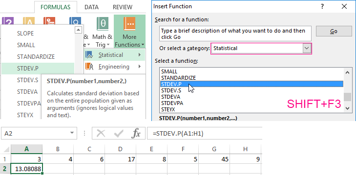
The standard deviation: the formula in Excel
There is a standard deviation in the entire population and in the sampling. In the first case, this is the square root of the general variance. In the second, this is a square root of the sampling variance.
A dispersion formula is compiled to calculate this statistical indicator. The square root is extracted from it. But in Excel, there is a ready-made function for finding the root-mean-square deviation.
The root-mean-square deviation is related to the scope of the initial data. This is not enough for a figurative representation of the variation of the analyzed range. The coefficient of variation is calculated to obtain the relative level of the data variability.
standard deviation / arithmetic mean
The formula in Excel is as follows:
STDEV.P (range of values) / AVERAGE (range of values).
The coefficient of variation is considered as a percentage. Therefore, set the percentage format in the cell set.