
Overview of formulas in Excel
Get started on how to create formulas and use built-in functions to perform calculations and solve problems.

Important: The calculated results of formulas and some Excel worksheet functions may differ slightly between a Windows PC using x86 or x86-64 architecture and a Windows RT PC using ARM architecture. Learn more about the differences.
Important: In this article we discuss XLOOKUP and VLOOKUP, which are similar. Try using the new XLOOKUP function, an improved version of VLOOKUP that works in any direction and returns exact matches by default, making it easier and more convenient to use than its predecessor.
Create a formula that refers to values in other cells
-
Select a cell.
-
Type the equal sign =.
Note: Formulas in Excel always begin with the equal sign.
-
Select a cell or type its address in the selected cell.

-
Enter an operator. For example, – for subtraction.
-
Select the next cell, or type its address in the selected cell.
-
Press Enter. The result of the calculation appears in the cell with the formula.


See a formula
-
When a formula is entered into a cell, it also appears in the Formula bar.
-
To see a formula, select a cell, and it will appear in the formula bar.


Enter a formula that contains a built-in function
-
Select an empty cell.
-
Type an equal sign = and then type a function. For example, =SUM for getting the total sales.
-
Type an opening parenthesis (.
-
Select the range of cells, and then type a closing parenthesis).
-
Press Enter to get the result.

Download our Formulas tutorial workbook
We’ve put together a Get started with Formulas workbook that you can download. If you’re new to Excel, or even if you have some experience with it, you can walk through Excel’s most common formulas in this tour. With real-world examples and helpful visuals, you’ll be able to Sum, Count, Average, and Vlookup like a pro.
Formulas in-depth
You can browse through the individual sections below to learn more about specific formula elements.
A formula can also contain any or all of the following: functions, references, operators, and constants.
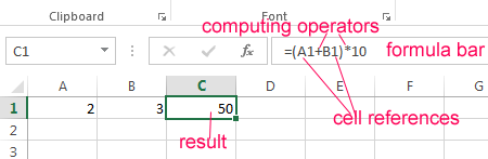
Parts of a formula

1. Functions: The PI() function returns the value of pi: 3.142…
2. References: A2 returns the value in cell A2.
3. Constants: Numbers or text values entered directly into a formula, such as 2.
4. Operators: The ^ (caret) operator raises a number to a power, and the * (asterisk) operator multiplies numbers.
A constant is a value that is not calculated; it always stays the same. For example, the date 10/9/2008, the number 210, and the text «Quarterly Earnings» are all constants. An expression or a value resulting from an expression is not a constant. If you use constants in a formula instead of references to cells (for example, =30+70+110), the result changes only if you modify the formula. In general, it’s best to place constants in individual cells where they can be easily changed if needed, then reference those cells in formulas.
A reference identifies a cell or a range of cells on a worksheet, and tells Excel where to look for the values or data you want to use in a formula. You can use references to use data contained in different parts of a worksheet in one formula or use the value from one cell in several formulas. You can also refer to cells on other sheets in the same workbook, and to other workbooks. References to cells in other workbooks are called links or external references.
-
The A1 reference style
By default, Excel uses the A1 reference style, which refers to columns with letters (A through XFD, for a total of 16,384 columns) and refers to rows with numbers (1 through 1,048,576). These letters and numbers are called row and column headings. To refer to a cell, enter the column letter followed by the row number. For example, B2 refers to the cell at the intersection of column B and row 2.
To refer to
Use
The cell in column A and row 10
A10
The range of cells in column A and rows 10 through 20
A10:A20
The range of cells in row 15 and columns B through E
B15:E15
All cells in row 5
5:5
All cells in rows 5 through 10
5:10
All cells in column H
H:H
All cells in columns H through J
H:J
The range of cells in columns A through E and rows 10 through 20
A10:E20
-
Making a reference to a cell or a range of cells on another worksheet in the same workbook
In the following example, the AVERAGE function calculates the average value for the range B1:B10 on the worksheet named Marketing in the same workbook.
1. Refers to the worksheet named Marketing
2. Refers to the range of cells from B1 to B10
3. The exclamation point (!) Separates the worksheet reference from the cell range reference
Note: If the referenced worksheet has spaces or numbers in it, then you need to add apostrophes (‘) before and after the worksheet name, like =’123′!A1 or =’January Revenue’!A1.
-
The difference between absolute, relative and mixed references
-
Relative references A relative cell reference in a formula, such as A1, is based on the relative position of the cell that contains the formula and the cell the reference refers to. If the position of the cell that contains the formula changes, the reference is changed. If you copy or fill the formula across rows or down columns, the reference automatically adjusts. By default, new formulas use relative references. For example, if you copy or fill a relative reference in cell B2 to cell B3, it automatically adjusts from =A1 to =A2.
Copied formula with relative reference
-
Absolute references An absolute cell reference in a formula, such as $A$1, always refer to a cell in a specific location. If the position of the cell that contains the formula changes, the absolute reference remains the same. If you copy or fill the formula across rows or down columns, the absolute reference does not adjust. By default, new formulas use relative references, so you may need to switch them to absolute references. For example, if you copy or fill an absolute reference in cell B2 to cell B3, it stays the same in both cells: =$A$1.
Copied formula with absolute reference
-
Mixed references A mixed reference has either an absolute column and relative row, or absolute row and relative column. An absolute column reference takes the form $A1, $B1, and so on. An absolute row reference takes the form A$1, B$1, and so on. If the position of the cell that contains the formula changes, the relative reference is changed, and the absolute reference does not change. If you copy or fill the formula across rows or down columns, the relative reference automatically adjusts, and the absolute reference does not adjust. For example, if you copy or fill a mixed reference from cell A2 to B3, it adjusts from =A$1 to =B$1.
Copied formula with mixed reference
-
-
The 3-D reference style
Conveniently referencing multiple worksheets If you want to analyze data in the same cell or range of cells on multiple worksheets within a workbook, use a 3-D reference. A 3-D reference includes the cell or range reference, preceded by a range of worksheet names. Excel uses any worksheets stored between the starting and ending names of the reference. For example, =SUM(Sheet2:Sheet13!B5) adds all the values contained in cell B5 on all the worksheets between and including Sheet 2 and Sheet 13.
-
You can use 3-D references to refer to cells on other sheets, to define names, and to create formulas by using the following functions: SUM, AVERAGE, AVERAGEA, COUNT, COUNTA, MAX, MAXA, MIN, MINA, PRODUCT, STDEV.P, STDEV.S, STDEVA, STDEVPA, VAR.P, VAR.S, VARA, and VARPA.
-
3-D references cannot be used in array formulas.
-
3-D references cannot be used with the intersection operator (a single space) or in formulas that use implicit intersection.
What occurs when you move, copy, insert, or delete worksheets The following examples explain what happens when you move, copy, insert, or delete worksheets that are included in a 3-D reference. The examples use the formula =SUM(Sheet2:Sheet6!A2:A5) to add cells A2 through A5 on worksheets 2 through 6.
-
Insert or copy If you insert or copy sheets between Sheet2 and Sheet6 (the endpoints in this example), Excel includes all values in cells A2 through A5 from the added sheets in the calculations.
-
Delete If you delete sheets between Sheet2 and Sheet6, Excel removes their values from the calculation.
-
Move If you move sheets from between Sheet2 and Sheet6 to a location outside the referenced sheet range, Excel removes their values from the calculation.
-
Move an endpoint If you move Sheet2 or Sheet6 to another location in the same workbook, Excel adjusts the calculation to accommodate the new range of sheets between them.
-
Delete an endpoint If you delete Sheet2 or Sheet6, Excel adjusts the calculation to accommodate the range of sheets between them.
-
-
The R1C1 reference style
You can also use a reference style where both the rows and the columns on the worksheet are numbered. The R1C1 reference style is useful for computing row and column positions in macros. In the R1C1 style, Excel indicates the location of a cell with an «R» followed by a row number and a «C» followed by a column number.
Reference
Meaning
R[-2]C
A relative reference to the cell two rows up and in the same column
R[2]C[2]
A relative reference to the cell two rows down and two columns to the right
R2C2
An absolute reference to the cell in the second row and in the second column
R[-1]
A relative reference to the entire row above the active cell
R
An absolute reference to the current row
When you record a macro, Excel records some commands by using the R1C1 reference style. For example, if you record a command, such as clicking the AutoSum button to insert a formula that adds a range of cells, Excel records the formula by using R1C1 style, not A1 style, references.
You can turn the R1C1 reference style on or off by setting or clearing the R1C1 reference style check box under the Working with formulas section in the Formulas category of the Options dialog box. To display this dialog box, click the File tab.
Top of Page


Need more help?
You can always ask an expert in the Excel Tech Community or get support in the Answers community.
See Also
Switch between relative, absolute and mixed references for functions
Using calculation operators in Excel formulas
The order in which Excel performs operations in formulas
Using functions and nested functions in Excel formulas
Define and use names in formulas
Guidelines and examples of array formulas
Delete or remove a formula
How to avoid broken formulas
Find and correct errors in formulas
Excel keyboard shortcuts and function keys
Excel functions (by category)
Need more help?
Want more options?
Explore subscription benefits, browse training courses, learn how to secure your device, and more.
Communities help you ask and answer questions, give feedback, and hear from experts with rich knowledge.
Excel formulas allow you to identify relationships between values in your spreadsheet’s cells, perform mathematical calculations with those values, and return the resulting value in the cell of your choice. Sum, subtraction, percentage, division, average, and even dates/times are among the formulas that can be performed automatically. For example, =A1+A2+A3+A4+A5, which finds the sum of the range of values from cell A1 to cell A5.
Excel Functions: A formula is a mathematical expression that computes the value of a cell. Functions are predefined formulas that are already in Excel. Functions carry out specific calculations in a specific order based on the values specified as arguments or parameters. For example, =SUM (A1:A10). This function adds up all the values in cells A1 through A10.
How to Insert Formulas in Excel?
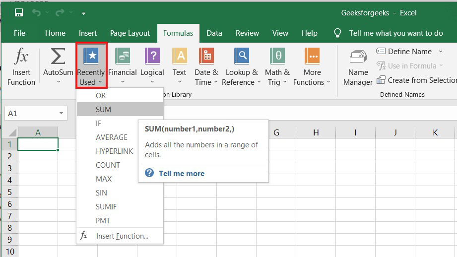
This horizontal menu, shown below, in more recent versions of Excel allows you to find and insert Excel formulas into specific cells of your spreadsheet. On the Formulas tab, you can find all available Excel functions in the Function Library:
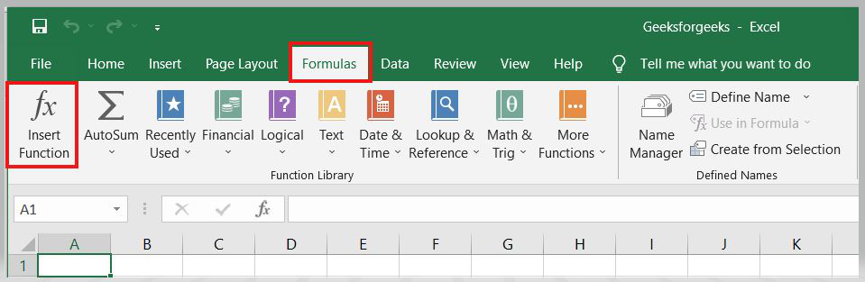
The more you use Excel formulas, the easier it will be to remember and perform them manually. Excel has over 400 functions, and the number is increasing from version to version. The formulas can be inserted into Excel using the following method:
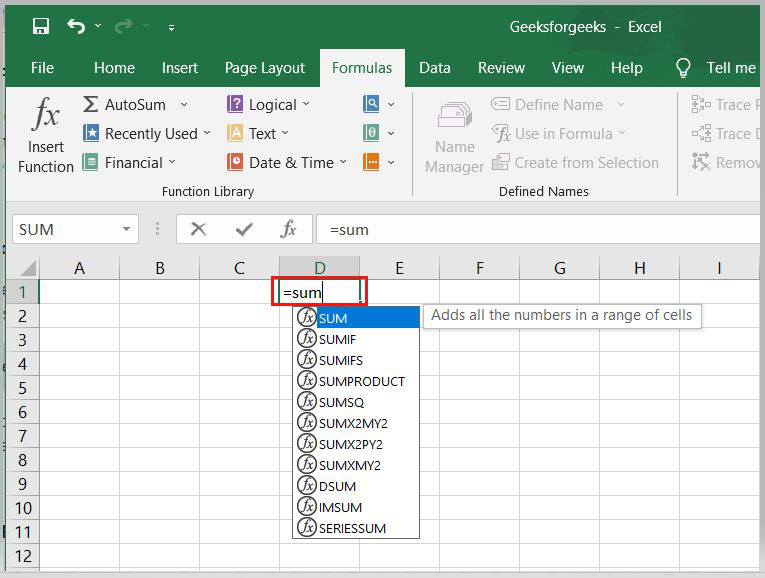
1. Simple insertion of the formula(Typing a formula in the cell):
Typing a formula into a cell or the formula bar is the simplest way to insert basic Excel formulas. Typically, the process begins with typing an equal sign followed by the name of an Excel function. Excel is quite intelligent in that it displays a pop-up function hint when you begin typing the name of the function.
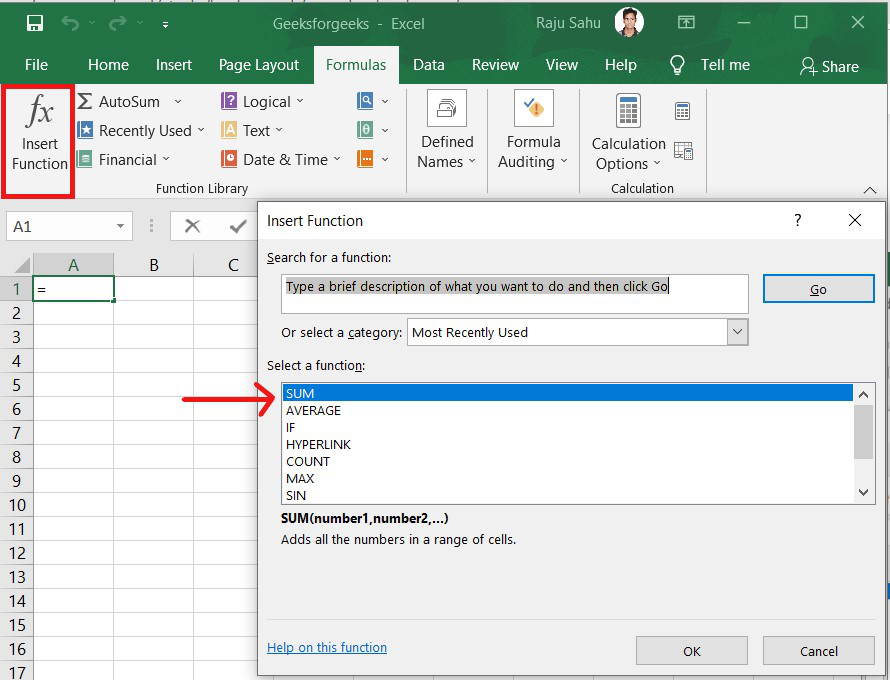
2. Using the Insert Function option on the Formulas Tab:
If you want complete control over your function insertion, use the Excel Insert Function dialogue box. To do so, go to the Formulas tab and select the first menu, Insert Function. All the functions will be available in the dialogue box.
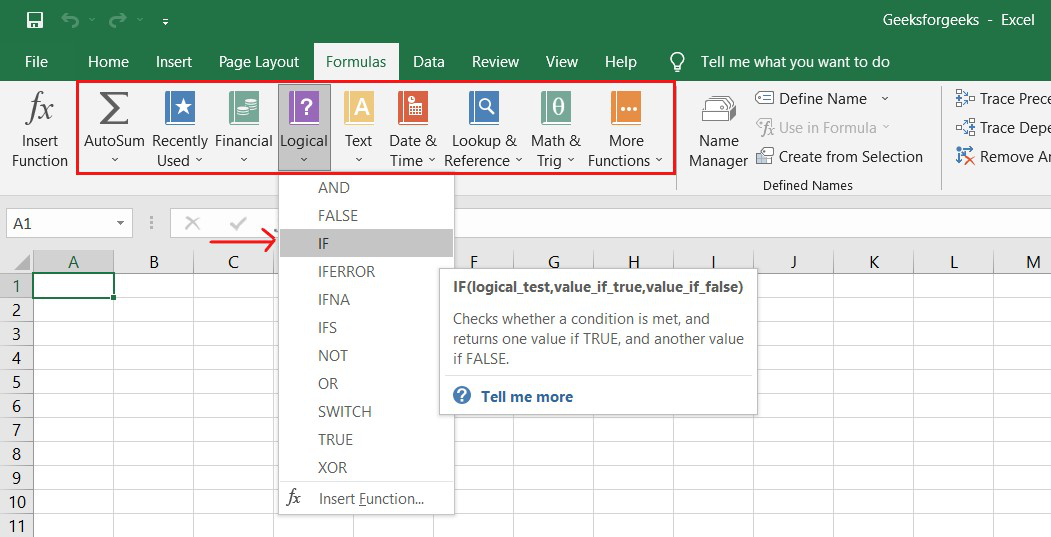
3. Choosing a Formula from One of the Formula Groups in the Formula Tab:
This option is for those who want to quickly dive into their favorite functions. Navigate to the Formulas tab and select your preferred group to access this menu. Click to reveal a sub-menu containing a list of functions. You can then choose your preference. If your preferred group isn’t on the tab, click the More Functions option — it’s most likely hidden there.
4. Use Recently Used Tabs for Quick Insertion:
If retyping your most recent formula becomes tedious, use the Recently Used menu. It’s on the Formulas tab, the third menu option after AutoSum.
Basic Excel Formulas and Functions:
1. SUM:
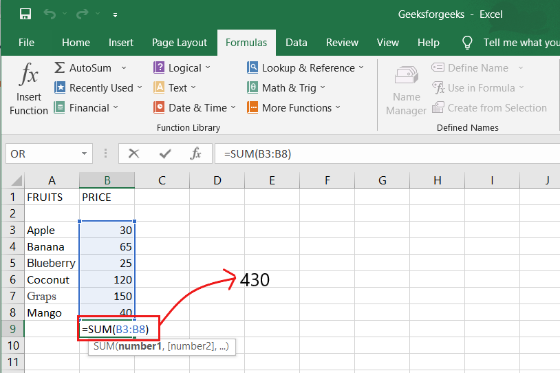
The SUM formula in Excel is one of the most fundamental formulas you can use in a spreadsheet, allowing you to calculate the sum (or total) of two or more values. To use the SUM formula, enter the values you want to add together in the following format: =SUM(value 1, value 2,…..).
Example: In the below example to calculate the sum of price of all the fruits, in B9 cell type =SUM(B3:B8). this will calculate the sum of B3, B4, B5, B6, B7, B8 Press “Enter,” and the cell will produce the sum: 430.
2. SUBTRACTION:
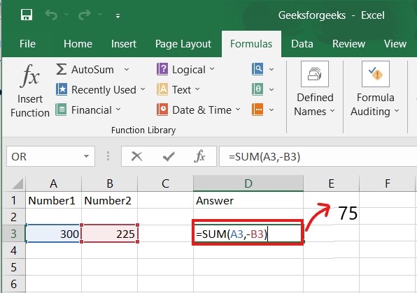
To use the subtraction formula in Excel, enter the cells you want to subtract in the format =SUM (A1, -B1). This will subtract a cell from the SUM formula by appending a negative sign before the cell being subtracted.
For example, if A3 was 300 and B3 was 225, =SUM(A1, -B1) would perform 300 + -225, returning a value of 75 in D3 cell.
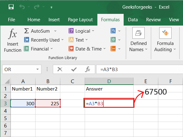
3. MULTIPLICATION:
In Excel, enter the cells to be multiplied in the format =A3*B3 to perform the multiplication formula. An asterisk is used in this formula to multiply cell A3 by cell B3.
For example, if A3 was 300 and B3 was 225, =A1*B1 would return a value of 67500.
Highlight an empty cell in an Excel spreadsheet to multiply two or more values. Then, in the format =A1*B1…, enter the values or cells you want to multiply together. The asterisk effectively multiplies each value in the formula.
To return your desired product, press Enter. Take a look at the screenshot above to see how this looks.
4. DIVISION:
To use the division formula in Excel, enter the dividing cells in the format =A3/B3. This formula divides cell A3 by cell B3 with a forward slash, “/.”
For example, if A3 was 300 and B3 was 225, =A3/B3 would return a decimal value of 1.333333333.
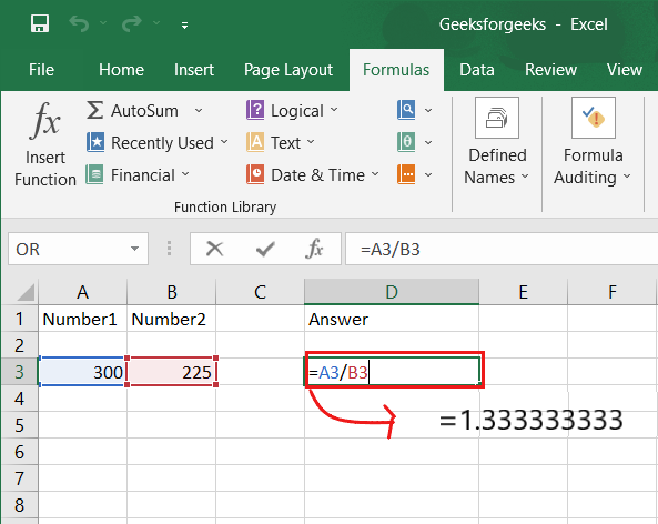
Division in Excel is one of the most basic functions available. To do so, highlight an empty cell, enter an equals sign, “=,” and then the two (or more) values you want to divide, separated by a forward slash, “/.” The output should look like this: =A3/B3, as shown in the screenshot above.
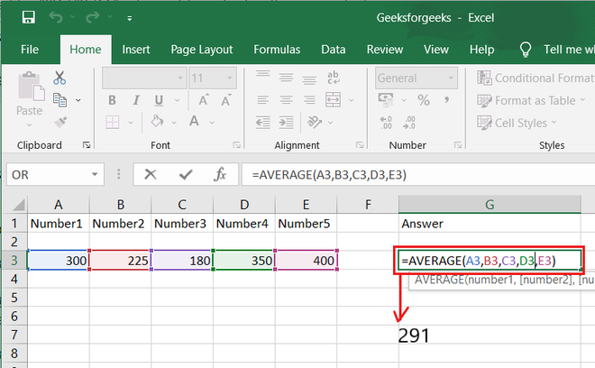
5. AVERAGE:
The AVERAGE function finds an average or arithmetic mean of numbers. to find the average of the numbers type = AVERAGE(A3.B3,C3….) and press ‘Enter’ it will produce average of the numbers in the cell.
For example, if A3 was 300, B3 was 225, C3 was 180, D3 was 350, E3 is 400 then =AVERAGE(A3,B3,C3,D3,E3) will produce 291.
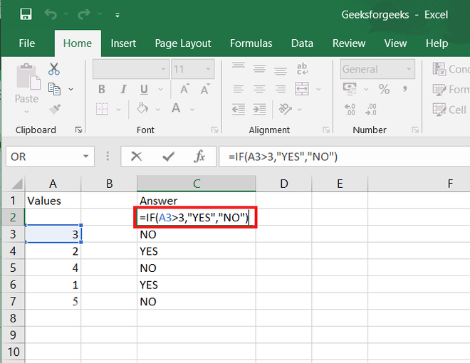
6. IF formula:
In Excel, the IF formula is denoted as =IF(logical test, value if true, value if false). This lets you enter a text value into a cell “if” something else in your spreadsheet is true or false.
For example, You may need to know which values in column A are greater than three. Using the =IF formula, you can quickly have Excel auto-populate a “yes” for each cell with a value greater than 3 and a “no” for each cell with a value less than 3.
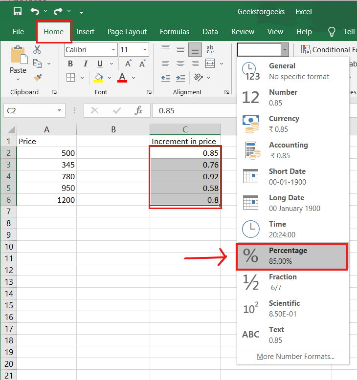
7. PERCENTAGE:
To use the percentage formula in Excel, enter the cells you want to calculate the percentage for in the format =A1/B1. To convert the decimal value to a percentage, select the cell, click the Home tab, and then select “Percentage” from the numbers dropdown.
There isn’t a specific Excel “formula” for percentages, but Excel makes it simple to convert the value of any cell into a percentage so you don’t have to calculate and reenter the numbers yourself.
The basic setting for converting a cell’s value to a percentage is found on the Home tab of Excel. Select this tab, highlight the cell(s) you want to convert to a percentage, and then select Conditional Formatting from the dropdown menu (this menu button might say “General” at first). Then, from the list of options that appears, choose “Percentage.” This will convert the value of each highlighted cell into a percentage. This feature can be found further down.
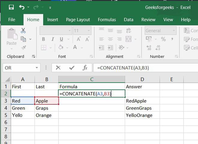
8. CONCATENATE:
CONCATENATE is a useful formula that combines values from multiple cells into the same cell.
For example , =CONCATENATE(A3,B3) will combine Red and Apple to produce RedApple.
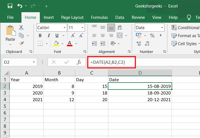
9. DATE:
DATE is the Excel DATE formula =DATE(year, month, day). This formula will return a date corresponding to the values entered in the parentheses, including values referred to from other cells.. For example, if A2 was 2019, B2 was 8, and C1 was 15, =DATE(A1,B1,C1) would return 15-08-2019.
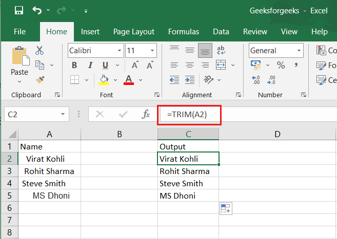
10. TRIM:
The TRIM formula in Excel is denoted =TRIM(text). This formula will remove any spaces that have been entered before and after the text in the cell. For example, if A2 includes the name ” Virat Kohli” with unwanted spaces before the first name, =TRIM(A2) would return “Virat Kohli” with no spaces in a new cell.
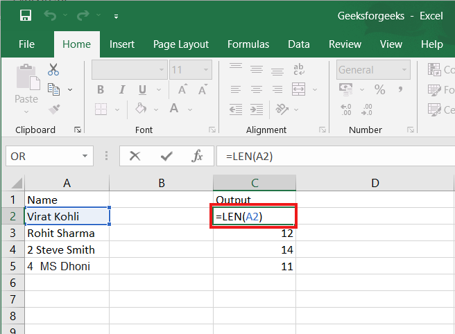
11. LEN:
LEN is the function to count the number of characters in a specific cell when you want to know the number of characters in that cell. =LEN(text) is the formula for this. Please keep in mind that the LEN function in Excel counts all characters, including spaces:
For example,=LEN(A2), returns the total length of the character in cell A2 including spaces.
The Excel Formulas Ultimate Guide
Introduction to Excel Formulas
In this guide, we are going to cover everything you need to know about Excel Formulas. Learning how to create a formula in Excel is the building block to the exciting journey to become an Excel Expert. So, let’s get started!
What is an Excel Formula?
Excel Formulas are often referred to as Excel Functions and it’s no big deal but there is a difference, a function is a piece of code that executes a predefined calculation, and a formula is an equation created by the user.
A formula is an expression that operates on values in a cell or range of cells. An example of a formula looks like this: = A2 + A3 + A4 + A5. This formula will result in the sum of the range of values from cell A2 to cell A5.
A function is a predetermined formula in Excel. It shows calculations in a particular order defined by its parameters. An example of a function is =SUM (A2, A5). This function will also provide the addition of values in the range of cells from A2 to A5 but here instead of specifying each cell address we are using the SUM function.
How To Write Excel Formulas
Let’s look at how to write a formula on MS Excel. To begin with, a formula always starts with a ‘+’ or ‘=’ sign, if you start writing the formula without any of these two signs, Excel will treat the value in that cell as text and will not perform any function.
In the screenshot below, you need to calculate the total sales amount by multiplying quantity sold with unit price. Select cell D2, type the formula ‘=B2*C2’ and press Enter. The result will display on cell D2.

Apply A Formula To An Entire Column Or Range
To copy a formula to adjacent cells, you can do the following:
- Select the cell with the formula and the adjacent cells you want to fill, then drag the fill handle.

- Select the cell with the formula and the adjacent cells you want to fill, then press Ctrl+D to fill the formula down in a column, or Ctrl+R to fill the formula to the right in a row.
- Select the cell with the formula and the adjacent cells you want to fill, then Click Home > Fill, and choose either Down, Right, Up, or Left.

How to Copy A Formula And Paste It
Excel allows you to copy the formula entered in a cell and paste it on to another cell, which can save both time and effort. To copy paste a formula:
- Select the cell whose formula you wish to copy
- Press Ctrl + C to copy the content
- Select the cell or cells where you wish to paste the formula. The copied cells will now have a dashed box around them.
- Press Alt + E + S to open the paste special box and select ‘Formula’ or Press “F’ to paste the formula.

- The formula will be pasted into the selected cells.
Basic Excel Formulas
Let’s start off with simple Excel Formulas. In the screenshot below, there are two columns containing numbers and we would like to use different operators like addition, subtraction, multiplication, and division on those to get different results. Excel uses standard operators for formulas, such as a plus sign for addition (+), a minus sign for subtraction (-), an asterisk for multiplication (*), a forward slash for division (/).

- Addition– To add values in the two columns, simply type the formula =A2+B2 on cell C2 and then copy paste the same on the cells below.
- Subtraction – To subtract values in Column B from Column A, simply type the formula =B2-A2 on cell C2 and then copy paste the same on the cells below.
- Multiplication – To multiply values in the two columns, simply type the formula =A2*B2 on cell C2 and then copy paste the same on the cells below.
- Division – To divide values in Column a by values in Column B, simply type the formula =A2/B2 on cell C2 and then copy paste the same on the cells below.
We can also calculate the percentage using Excel Formulas. In the image below, we have sales in Year 1 and Year 2 and we would like to know the % growth in sales from Year 1 to Year 2.

To do that, select cell C2 and type the formula = (B2 – A2)/B2*100
Basic Excel Functions
A function is a predefined formula that performs calculations using specific values in a particular order. Excel includes many common functions that can be useful for quickly finding the sum, average, count, maximum value, and minimum value for a range of cells. a function must be written a specific way, which is called the syntax.
The basic syntax for a function is an equals sign (=), the function name, and one or more arguments. A Function is generally comprised of two components:
1) A function name -The name of a function indicates the type of math Excel will perform.
2) An argument – It is the values that a function uses to perform operations or calculations. The type of argument a function uses is specific to the function. Common arguments that are used within functions include numbers, text, cell references, and names
Let’s look at some common Excel Functions:
SUM Function
The SUM formula adds 2 or more numbers together. You can use cell references as well in this formula.
Syntax: =SUM(number1, [number2], …)
Example: =SUM(A2:A8) or SUM(A2:A7, A9, A12:A15)

AUTOSUM Function
The AutoSum command allows you to automatically insert the most common functions into your formula, including SUM, AVERAGE, COUNT, MIN, and MAX.
Select the cell where you want the formula, Go to Home > Click on AutoSum > From the dropdown click on “Sum” > Enter.

COUNT Function
If you wish to how many cells are there in a selected range containing numeric values, you can use the function COUNT. It will only count cells that contain either numbers or dates.
Syntax: =COUNT(value1, [value2], …)
In the example below, you can see that the function skips cell A6 (as it is empty) and cell A11 (as it contains text) and gives you the output 9.
COUNTA Function
Counts the number of non-empty cells in a range. It will include cells that have any character in them and only exclude blank cells.
Syntax: =COUNTA(value1, [value2], …)
In the example below, you can see that only cell A6 is not included, all other 10 cells are
counted.

AVERAGE Function
This function calculates the average of all the values or range of cells included in the parentheses.
Syntax: =AVERAGE(value1, [value2], …)

ROUND Function
This function rounds off a decimal value to the specified number of decimal points. Using the ROUND function, you can round to the right or left of the decimal point.
Syntax: =ROUND(number,num_digit)
This function contains 2 arguments. First, is the number or cell reference containing the number you want to round off and second, number of digits to which the given number should be rounded.
- If the num-digit is greater than 0, then the value will be rounded to the right of the decimal point.
- If the num-digit is less than 0, then the value will be rounded to the left of the decimal point.
- If the num-digit equal to 0, then the value will be rounded to the nearest integer.


MAX Function
This function returns the highest value in a range of cells provided in the formula.
Syntax: =MAX(value1, [value2], …)
In the example below, we are trying to calculate the maximum value in the dataset from A2 to A13. The formula used is =MAX(A2: A13) and it returns the maximum value i.e. 96.251

MIN Function
This function returns the lowest value in a range of cells provided in the formula.
Syntax: =MIN(value1, [value2], …)
In the example below, we are trying to calculate the minimum value in the dataset from A2 to A13. The formula used is =MIN(A2: A13) and it returns the minimum value i.e. 24.178

TRIM Function
This function removes all extra spaces in the selected cell. It is very helpful while data cleaning to correct formatting and do further analysis of the data.
Syntax: =trim(cell1)
In the example below, you can see the name in cell A2 contains an extra space, in the beginning, =TRIM(A2) would return “Steve Peterson” with no spaces in a new cell.

Advanced Excel Formulas
Here is a list of Excel Formulas that we would feel comfortable referring to as the top 10 Excel Formulas. These formulas can be used for basic problems or highly advanced problems as well, though advanced excel formulas are nothing but a more creative way of using the formulas. Sure, there are legitimate Advanced Excel Formulas such as Array Formulas but in general the more advanced the problem, the more creative you need to be with Formulas.
Currently, Excel has well over 400 formulas and functions but most of them are not that useful for corporate professionals so here is a list that we believe contains the 10 best Excel formulas.
Starting with number 10 – it’s the IFERROR formula
- IFERROR Function –
- SUBTOTAL Function –
- SMALL/LARGE Function –
- LEFT Function –
- RIGHT Function –
- SUMIF Function –
- MATCH Function –
- INDEX Function –
- VLOOKUP Function –
- IF Function –
IFERROR Function –
You ever have presented a worksheet that you thought was perfect but were surprised with a “#DIV /0!” error or an “#N/A” error message (See the screenshot below), then this function is perfect for you. Excel has an “IFERROR” function that can automatically replace error messages with a message of your choice.

The IFERROR function has two parameters, the first parameter is typically a formula and the second parameter, value_if_error, is what you want Excel to do if value, the first parameter, results in an error. Value_if_error can be a number, a formula, a reference to another cell, or it can be text if the text is contained in quotes.
That means you can put formula or an expression in the first part of the IFERROR function and Excel will show the result of that formula unless the formula results in an error. If the formula results in an error, Excel will follow the instructions in the second half of the IFERROR formula.
This function cleans up your sheet and it will visually make things look a lot better and more professional.
Let’s see an example to make the concept clearer.

In this example, we have two lists – one contains the names of all people (Column A) and the second list contains the name of award winners only (Column F).
We have used a simple Vlookup function to see if the name is an award winner. The Vlookup function (it is covered later in details) will search the list on the right, if the name is present in the award winner list, it will show the name or else it will show an error.
The N/A error makes the worksheet look dirty and unprofessional. Now we will add iferror function here to remedy the same.
=IFERROR(VLOOKUP(A5,$F$5:$F$10,1,0),””)

IFERROR function will recognize the error and instead of displaying the error message will display the text, say a blank, or you can show any other message that you desire.
IFERROR is a great way to replace Excel-generated error messages with explanations, additional information, or simply leave the cell blank.
SUBTOTAL Function –
The SUBTOTAL function returns the aggregate value of the data provided. You can select any of the 11 functions that SUBTOTAL can calculate like SUM, COUNT, AVERAGE, MAX, MIN, etc. SUBTOTAL Function can also include or exclude values in hidden rows based on the input provided in the function.
Excel’s traditional formulas do not work on filtered data since the function will be performed on both the hidden and visible cells. To perform functions on filtered data one must use the subtotal function.
Syntax: SUBTOTAL(function_num,ref1,…)The first parameter is the name of the function to be used within the subtotal function and the second parameter is the range of cells that should be subtotalled
The list of functions that can be used in given below. If the data is filtered manually, the numbers from 1 – 11 will include the hidden cells and number from 101 – 111 will exclude them.

Let’s understand this function with an example.

Here we have a list of name of person, with their country and the total sales they have achieved in Q1. We will use the subtotal function to calculate the total sales in cell C26. We will also select the function in such a way that it works on filtered data as well.
The formula will be =SUBTOTAL (109,C5:C24)

This will display the total sales. Now, we filter the data to see the sales made by people in US only. You will see the value in the cell containing the SUBTOTAL function updates and it filters the dataset and displays the total sales made by US only.

Here is another benefit of using a SUBTOTAL function:
When you’re creating an information summary, especially like a profit and loss statement where you’ve got lots of subtotals, what you can do is you can use the subtotal formula, and then at the end, you can put a big old formula right at the end and it will just ignore your subtotal.
Here we have 4 different tables for sales in 4 different countries.

We can add individual SUBTOTAL functions for each table and then a grand total function in the end. The SUBTOTAL function in the end will ignore all the other SUBTOTAL functions above it and will provide you the total sales.

SMALL/LARGE Function –
Here, we have two formulas and they’re two sides of the same coin – the small formula and the large function. So, imagine you’ve got a list of, let’s say, sales data or cost data and what SMALL Function will do is provide you with the smallest value in the data set. You can also specify if you want the first smallest or second smallest. Similarly, with the large formula, you can extract the largest value in this dataset, the second largest and so on.
Syntax: =LARGE(array,k); SMALL(array,k)
The first parameter is the range of data for which you want to determine the k-th largest value and the second is the position (from the largest/smallest) in the cell range of the value to return.

Now, in the dataset above if you want to know the person who has achieved the highest sales, you can use the LARGE function – =LARGE($C$4:$C$23,E5). We have used E5 for the second parameter as it contains the value 1. If we copy paste the formula in the cells below, you will get the 1st, 2nd, 3rd, 4th and 5th largest value in the dataset. Similarly, we have used the function SMALL to get the value for lowest sales.

LEFT & RIGHT Function –
A lot of people work on text manipulation with functions like text to columns or even do it manually but being able to extract the exact number of characters that you want from the left or the right side of a string is absolutely invaluable. This is what the LEFT and RIGHT function does – it extracts a given number of characters from the left/right side of a supplied text string.
Syntax: =LEFT (text, [num_chars]) and RIGHT(text,num_chars)
The first parameter is the text string containing the characters you want to extract and the second parameter specifies how many characters you want LEFT/RIGHT to extract; 1 if omitted.
In the example given below, we have full names of people and we would like to extract the first name. We can surely do it using text to column, but using the LEFT function will give us a more automated result. So, let’s see how it can be done.

When you look at the data, you can see that a character is common in all names and it separates the first name and last name – it is a “space”. If we can find out the position of space in each cell, we can easily extract the first name.
Does Excel have a formula for this as well? Off course! SEARCH is the function that will come to your rescue.
SEARCH function provides the position of the first occurrence of the specified character.SEARCH (find_text, within_text, start_num) has three parameters – first is the character you want to find, second is the text in which you want to search and third is the character number in Within_text, counting from the left, at which you want to start searching. If omitted, 1 is used.
So, going back to our example, we use the formula SEARCH to find the position of the character – space in Column A. We will need to subtract “1” from the position to get the desired result. The formula will be =SEARCH (“ “,A5)-1 and copy paste it down.

Now we will use the LEFT Function to get the first name. =LEFT(A5,B5) – A5 contains the full name and B5 contains the number of characters from left that contains the first name.

SUMIF(S) Function –
This function is used to conditionally sum up a range of values. It returns the summation of selected range of cells if it satisfies the given criteria. It is like the SUM function because it adds stuff up. But, it allows us to specify conditions for what to include in the result. Criteria can be applied to dates, numbers, and text using logical operators (>,<,<>,=) and wildcards (*,?) for partial matching. For example, SUMIF function can add up the quantity column, but only include those rows where the SKU is equal to, say A200.
Syntax: =SUMIF (range, criteria, [sum_range])
The first argument is the range of values to be tested against the given criteria, second argument is the condition to be tested against each of the values and the last argument is the range of numeric values if the criteria is satisfied. The last argument is optional and if it is omitted then values from the range argument are used instead.
SUMIF can handle one criterion only. For multiple conditional summing – we can use SUMIFS.
The Syntax of this function is =SUMIFS( sum_range, criteria_range1, criteria1, [criteria_range2, criteria2], … ); where sum_range is the range of values to add, criteria_range1 is the range that contains the values to evaluate and criteria1 is the value that criteria_range1 must meet to be included in the sum. You can add additional pairs of criteria range and criteria if further conditions are to be met.
It is advisable to use SUMIFS even if you have only one criteria to evaluate as it will help you to easily modify the function if additional conditions come up over time.
Let’s dive into an example. Below we have data containing name, country in which sales were made, and the different quarterly sales data.

Using SUMIFS function, we would like to calculate the sum of sales in Q1 for the different countries. Now, to get the total sales in UK in Q1, we select the cell I4 and type the formula =SUMIFS(C4:C23,B4:B23,H4). We will then copy paste the formula below to get the result for each country.

INDEX & MATCH Function –
The MATCH function is used to search for an item and return the relative position of that item in a horizontal or vertical list.
Syntax: MATCH(lookup_value, lookup_array, [match_type])
The first argument is the value you want to look up, second is the range of cells being searched and the last argument, which is optimal, tells the MATCH function what sort of lookup to do.
The three acceptable values for match type are 1, 0 and -1. The default value for this argument is 1.
- If the input is 1. MATCH finds the largest value that is less than or equal to the lookup_value. The values in the lookup_array argument must be placed in ascending order.
- If the input is 0. MATCH finds the first value that is exactly equal to the lookup_value. The values in the lookup_array argument can be in any order.
- If the input is -1. MATCH finds the smallest value that is greater than or equal to the lookup_value. The values in the lookup_array argument must be placed in descending order.
For example, if the range A1:A5 contains the values Evelyn Greer, Randy Mueller, Maverick Cooper, Eesha Bevan and Nancie Velez, then the formula =MATCH(“Maverick Cooper”,A1:A5,0) returns the number 3, because Maverick Cooper is the third item in the range.

INDEX
function is used to return the value in the cell based on the row number and column number provided. It can do two-way lookup: where we are retrieving an item from a table at the intersection of a row header and column header.
Syntax: =INDEX (array, row_num, [col_num])
The first argument is the range/array containing the values you want to look up, second is the row number; the row number from which the value is to be fetched (if omitted, Column_num is required) and third is the column number from which the value is to be fetched.
For Example: =INDEX(A1:B6,3,2)
This function will look in the range A1 to B6, and It will return whatever value is housed in Row 3 and Column 2. The answer here will be “India” in cell B3.

As you have seen, Index and Match on their own are effective and powerful formulas but together they are absolutely incredible. Let’s look at it.
Remember that you must tell INDEX Function which row and column number to go to. In the examples above, we hard coded it to a specific number. But instead, we can drop this MATCH function into that space in our formula and make the formula dynamic.
Let’s dive into an example.

Here we have two dropdowns in cell H9 and H11 containing names and quarters. What we want is that, once we select a name in cell H9 and a quarter in cell H11, the corresponding sales for the specified person and quarter appears in cell H14. We will be using INDEX & MATCH to accomplish this.The formula will be: =INDEX($A$3:$F$23,MATCH(H9,$A$3:$A$23,0),MATCH(H11,$A$3:$F$3,0))

This function will take A3:F23 as the range and the first match will use the name mentioned in cell H9 (here, Eesha Bevan) and obtain the position of it in the Name column (A3:A23). This becomes the row number from which the data needs to be taken. Similarly, the second match will use the quarter mentioned in cell H11 (here, Q2 Total Sales) and obtain the position of it in the Quarter’s row (A3:F3). This becomes the column number from which the data needs to be taken. Now, based on the row and column number provided by the Match functions, index function will now provide the required value, i.e. 18,250.
This formula is now dynamic, i.e. if you change the name or quarter in cells H9 or H11 the formula will still work and provide the correct value.
VLOOKUP Function –
This function is not as flexible or powerful as the combination of Index and Match that we talked about just now, however, the reason this is number 2 on the list is simply because it’s quick, flexible, easy to implement and doesn’t put a whole lot of strain on your CPU while calculating.
Vlookup is a vertical lookup function that tries to match a value in the first column of a lookup table and then return an item from a subsequent column.
Syntax: VLOOKUP ( lookup_value , table_array , col_index_num , [range_lookup] )
- Lookup_value: Is the value to be found in the first column of the table, and can be a value, a reference, or a text string.
- Table_array: This is the lookup table and the first column in this range must contain the lookup_value.
- Col_index_num: This is the column number in table_array from which the matching value should be returned.
- Range_lookup: is a logical value that tells you the type of lookup you want to do. To find the closest match in the first column (sorted in ascending order) use TRUE; to find an exact match use FALSE (if omitted, TRUE is used as default).

In the example above, the first table contains name, country and quarterly sales and the second table contains the country name and nationality.
Now, we have an empty column (Column G) in the first table and we want to use Vlookup to extract the nationality of a person based on the country name mentioned in Column B.

The function will be: =VLOOKUP(B4,$K$3:$L$7,2,0). This function will lookup the value in cell B4 (i.e. UK) in the first column of the range K3:L7 and will return the corresponding value from the second column of the range i.e. British.
IF Function
So, why is this formula so important? Simply because this function gives you the flexibility to control your outcomes. When you can understand and model your outcomes, you can create logic and thus create a business model.
IF function is a logical test that evaluates a condition and returns a value if the condition is met, and another value if it is not met.
Syntax: =IF(logical_test,[value_if_true],[value_if_false])
- Logical test – It is condition that needs to be evaluated. The logical operators that can be used are = (equal to), > (greater than), >= (greater than or equal to), < (less than), <= (less than or equal to) and <> (not equal to).
- Value_if_true – Is the value that is returned if Logical_test is TRUE. If omitted, TRUE is returned.
- Value_if_false – Is the value that is returned if Logical_test is FALSE. If omitted, FALSE is returned.
You can also use OR and AND functions along with IF to test multiple conditions. Example: =IF(AND(logical_test1, logical_test2),[value_if_true],[value_if_false]).
IF functions can also be nested, the FALSE value being replaced by another IF function to make a further test. Example: =IF(logical_test,[value_if_true,IF(logical_test,[value_if_true],[value_if_false])).
Let’s go through the IF function with an example to discuss it in detail.

In the screenshot above, we have a table that contains the name, country and quarterly sales achieved by different persons. Now, we want to see which persons have been promoted based on the criteria that the total sales achieved by that person is greater than £250,000. In the column for Promotions (Column G), we want the formula to test whether the total sales are greater than £250,000, if it is true then we want the text “Promoted” to be displayed, else a blank.
The formula to be used will be: =IF(C4+D4+E4+F4>250000,”Promoted”,””)

So, this completes our Top 10 Excel formulas. As we have already mentioned there are 400+ Excel formulas available and these 10 best Excel formulas will cover about 70% to 75% of your needs, but if you want to go a little bit more we have a book about the 27 best Excel formulas that will cover pretty much all of your formula requirements. The best thing about this is – it contains info-graphics and is completely free!
Excel Formulas Not Working: Troubleshooting Formulas
Continuing our series on Excel Formulas, this part is all about troubleshooting Excel Formulas. Let’s look at the major issues.
How To Refresh Excel Formulas
If Your Excel Formulas are Not Calculating, then start off by refreshing them. Do either of the following methods to refresh formulas:
- Press F2 and then Enter to refresh the formula of a particular cell.
- Press Shift + F9 to recalculate all formulas in the active sheet or you can go to the Formula Tab > Under Calculation Group > Select “Calculate Sheet”.

- Press F9 to recalculate all formulas in the workbook or you can go to the Formula Tab > Under Calculation Group > Select “Calculate Now”.

- Press Ctrl + Alt + F9 to recalculate formulas in open worksheets of all open workbooks.
- Press Ctrl + Alt + Shift + F9 to recalculate formulas in all sheets in all open workbooks.
How To Show Formulas In Excel
Usually when you type a formula in Excel and press Enter, Excel displays a calculated value in the cell. If you wish to see the formula that you have typed in the cell, you can do either of the following methods:
- Go to Formula Tab > Under Formula Auditingsection > Click on “Show Formulas”.

- Press Ctrl + ` to show formulas in the cell.

How To Audit Your Formula
Formula Auditing is used in Excel to display the relationship between formulas and cells. There are different ways in which you can do that. Let’s cover each one in detail:
- Trace Precedents
Trace Precedents shows all the cells that affect the formula in the selected cell. When you click this button, Excel draws arrows to the cells that are referred to in the formula inside the selected cell.

In the example below, we have a cost table that contains totals and grand total. We will now use trace precedents to check how the cells are linked to each other.Click on the cell containing grand total (Cell C15) > Go to Formula Tab > Click on “Trace Precedents”.

To see the next level of precedents, click the Trace Precedents command again.

To remove arrows, simply go to Formula Tab > Click on “Remove Arrows”.

- Trace Dependents
Trace Dependents show all the cells that are affected by the formula in the selected cell. When you click this button, Excel draws arrows from the selected cell to the cells that use, or depend on, the results of the formula in the selected cell.

In the example below, we have a cost table that contains totals and grand total. We will now use trace dependents to check how the cells are linked to each other.Click on the cell containing Property Cost (Cell C3) > Go to Formula Tab > Click on “Trace Dependents”.

To see the next level of dependents, click the Trace Dependents command again

- Evaluate Formula
This function is used to evaluate each part of the formula in the current cell. The Evaluate Formula feature can be quite useful in formulas that nest many functions within them and helps in debugging an error.

To evaluate the calculation in cell C15 (Grand Total), Click on the cell > Go to Formula Tab > Click on “Evaluate Formula”.

A dialog box will appear that will enable you to evaluate parts of the formula.


This will help you to debug an error as it provides you with the value calculated at each step of evaluation done by Excel.
- Error Checking
This function is helpful as it is used to understand the nature of an error in a cell and to enable you to trace its precedents.

To check for the errors shown in the screenshot below, click on cell C18 > Click on Formula Tab > Under Formula Auditing group > Click on “Error Checking”.

Once you click on Error Checking button, a dialog box will appear. It will describe the reason for the error and will guide you on what to do next. You can either trace the error or ignore the error or go to the formula bar and edit it. You can choose either of these options by clicking on the button shown in the Error Checking Dialog box.

These top formulas and functions of Excel will surely help and guide you in every step of your Excel Journey.
The formula prescribes to the program Excel the procedure with numbers, the values in the cell or group of cells. Without formulas spreadsheets are not needed in principle.
The structure of formula includes: constants, operators, references, functions, range names, parentheses are contained arguments of other formulas. Let us consider the practical application of the formulas for newcomer users.
The formulas in excel for dummies
For setting the formula for the cell, it is necessary to activate it (to put the cursor) and insert the equal sign (=). Similarly you can insert the equal sign in the formula bar. After putting, press Enter. The result of calculations will appear in the cell.
In Excel employs standard mathematical operators:
| Operator | Operation | Example |
| + (Plus sign) | Addition | =В4+7 |
| — (Minus sign) | Subtraction | =А9-100 |
| * (Asterisk) | Multiplication | =А3*2 |
| / (Slash) | Division | =А7/А8 |
| ^ (Circumflex) | Degree | =6^2 |
| = (Equal sign) | Equal | |
| < | Less | |
| > | More | |
| <= | Less than or equal | |
| >= | Greater or equal | |
| <> | Not Equal |
The symbol «*» is used necessarily during multiplying. To pass it, as it is accepted in written arithmetic calculation is unacceptable. That is the record (2+3)5 Excel won’t understand.
The program Excel can be used as a calculator. That is insert numbers in the formula and operators of mathematical calculation and get the result immediately.

But more often entered addresses of cells. That is, a user enters the reference of the cell with the meaning which will operate the formula.
During changing the values in the cells the formula automatically recalculates the result.
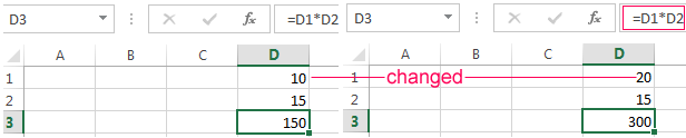
References can be combined in one formula with simple numbers.
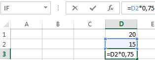
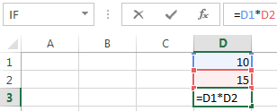
The operator multiplies the importance of B2 in 0,75.
In our example:
- Insert the cursor in B3 and enter «=».
- Click on the cell B2 – Excel it (the name of cell appeared in the formula, around the cell formed a rectangle).
- Input the symbol «*», setting 0. 5 from the keyboard and pressed ENTER.
If in the same formula is used several operators, the program will process them in the following order:
- %, ^;
- *, /;
- +, -.
For changing the sequence you may by parentheses: in the first order Excel calculates the cost of the expression in parentheses.
How in the excel formula to assign the constant cell
There are 2 types of cell references: relative and absolute ones. When copying the formula those references reveal itself in different ways: the relative references changing, absolute references remain constant.
All cell references the program considers as relative, if the user has not settled another criterion. With relative references you may multiplied the same formula to several rows or columns.
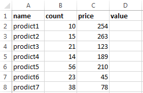
- Manually complete in the first graphs of the training table. We have this option:
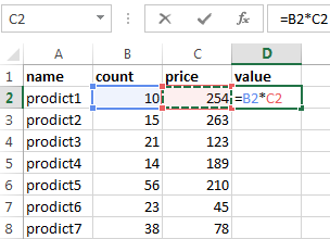
- Recollect from math: to determine the cost of a few items, you need the price for 1 unit multiplied on the quantity. For calculating the cost, need to enter a formula in the cell D2: = unit price * quantity. Constants formula – are cell references with the appropriate importance’s.
- Push ENTER – and the program displays the importance of the multiplication. The same procedure should be done for all cells. How in Excel to install the formula for a column? You need to copy the formula from the first cell in other rows. Relative references — in helping ones.
To find in the lower right corner of D2 of the column the marker of autocomplete. You need to click on this point with the left mouse button, hold it and down the column.
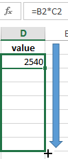
In order to release the mouse button — the formula is copied to selected cells with relational references. That is, in each cell will be the formula with their argument.
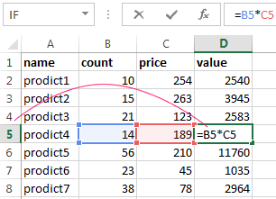
Links in the cell are associated with the line.
Formula with the absolute reference refers to the same cell. That is when you AutoFill or copy something, the constant is unchanged (or constant).
For pointing to Excel on the absolute reference, the user must place a dollar sign ($). The easiest way to do this with helping the F4 key.
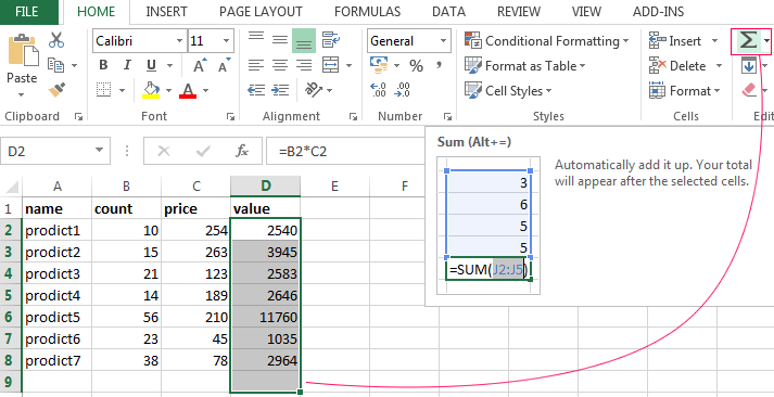
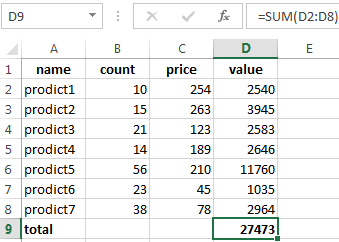
- Create a row «total». Find the total cost of all goods. Allocate numerical relevance’s of the amount column «value», plus one more cell. This is the range D2:D9.
- Use the autocomplete function. The button «AutoSum» is on the tab «HOME» in the tool group «Editing».
- After clicking on the icon «AutoSum» (or combination of keys ALT+ «=») folding the selected number and displaying the result in the empty cell.
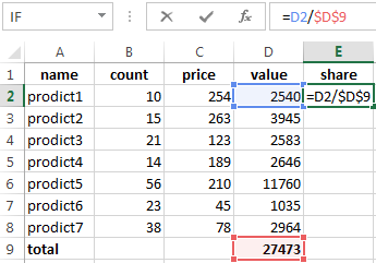
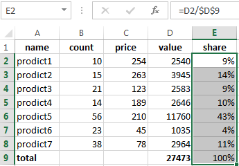
Create one more column, where we calculate the share of each good in the total cost. To do this:
- Devide the cost of a single product on the cost of all goods and multiply the result by 100. The cell reference with the meaning of of the total cost must to be absolute, that at copying it will stay unchanged.
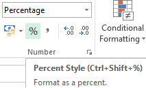
- To get percents in Excel, don`t have to multiply the quotient on 100. Allocate the cell with the result and press «Percent Style» (CTRL+SHIFT+%). Or press the hot key combination: CTRL+SHIFT+5.
- Copy the formula throughout the entire column: only changes the first calculated value in the formula (a relative reference). The second one (an absolute reference) remains the same. To test the correctness of calculations and to find the result. 100%. All right.
When creating formulas, used the following formats of absolute links:
- $B$2 – when copying column and row stay constant;
- B$2 – when copying a string stay constant;
- $B2 – the column is not changed.
How to make the table in excel with formulas
For saving time with the introduction of similar formulas in table cells, applyed the markers autocomplete. If you need to fix the link, make it absolute. For changing the values during copy a relative reference.
The simplest formulas of filling tables in Excel:
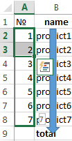
- Before the names of goods we will put one more column. Allocated to any cell in the first column, click with the right mouse button. Click «Paste». Or press at first the key combination CTRL+SPACEBAR to choose an total column of the sheet. And then the combination: CTRL+SHIFT+«+» to insert a column.
- Let’s call the new column «№». Put in A1 number «1», A2 – «2». To allocate the first two cells with the left mouse button the marker autocomplete – pull down.
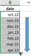
- The same rule may be filled, for example, dates. If the intervals between them the same – a day, a month, an year. Enter in G1 «oct.15», in the second «nov.15». To allocate the first two cells and for a marker down.
- To find the average price of the goods. Allocate the column with the prices + one more cell. Open menu of button «AutoSum» – select a formula for auto calculation of the average value.
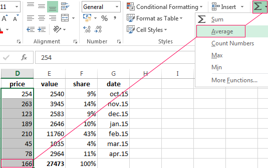
To test the correctness, make double-click on the result.
Formulas in Excel for dummies: rules of introduction, operators, using of absolute and relative references. How to set formula for column? Autocomplete of the tables.

How to Create a Simple Formula in Excel
To create a formula in excel must start with the equal sign “=”. If there is no equals sign, then whatever is typed in the cell will not be regarded as a formula.
Here’s how to create a simple formula, which is a formula for addition, subtraction, multiplication, and division. An addition formula using the plus sign “+”, subtraction formula using the negative sign “-“, a multiplication formula using an asterisk sign “*” and division formula using the slash “/”.
Addition Formula
There are two numbers in cell B1 and B2. How to create a formula in excel to add both of them?

There are several ways of writing a formula. The first way is using the keyboard and the arrow keys, the second way using the keyboard and mouse and a third way to use the keyboard by typing directly the formula and the address of cell involved.
For the above addition, the formula will be used the first way.
- Place the cursor in cell B4 and then type the equals sign “=”

- Press the up arrow button, point to cell B1, the cursor turns into dashed line.

- Type the plus sign “+” for the addition operation

- Press the up arrow button again, point to cell B2

- Press the ENTER key
The result is as shown below

Subtraction Formula
How to write a formula in excel for subtracting number1 by number2?. The reduction formula to use the second way, i.e. using the keyboard and mouse.
- Place the cursor in cell B5 and then type the equals sign “=”
- Click cell B1 using the mouse
- Type the negative sign “-” for the subtraction operation
- Click cell B2 using the mouse
- Press the ENTER key
For more details, you can see the animation below.
Multiplication Formula
How to make a formula in excel to multiply number1 by number2. For the multiplication formula using the third way of using the keyboard by writing directly the formula and the address of the cell involved.
- Place the cursor in cell B6 and then type the equals sign “=”
- Type B1
- Type an asterisk “*” for multiplication operations
- Type B2
- Press the ENTER key
For more details, you can see the animation below.
Division Formula
How to do formulas in excel to divide number1 with number2.
- Place the cursor in cell B7 and then type the equals sign “=”
- Point the cursor to cell B1
- Type a slash mark “/” for the division operation
- Point the cursor to cell B2
- Press the ENTER key
The result is as shown below

How to View Formulas in Excel
The easiest way to see the formula in a cell is to look at the formula bar. Point the cursor to a cell that contains a formula, then the formula bar will display the formula in the cell. The location of the formula bar is below the ribbon menu.

The picture above shows the formula contained in cell B4. To see formulas in other cells just move the cursor to the desired cell and see the formula in the formula bar.
Formula bar can only display formulas in the active cell, meaning only one formula can be shown. To be able to display all the formulas in a worksheet, please read the article below “How to Display Cell Formulas in Excel”
How to Edit Formula in Excel
There are two ways to edit a formula, using the F2 key or using a formula bar.
Editing with the F2 key
Place the cursor in the cell containing the formula, then press the F2 key. The contents of the formula will appear, and the cells involved in the formula will be marked with a colored box.
The picture below shows the existing addition formula in cell B4. There are two cells involved in the formula: cell B1 and B2. The address of the cell B1 light blue colored then the cell B1 will be surrounded with the same colored line, likewise with cell B2, the color of lines around it is same as cell B2 address color.

For example, the formula will be edited by adding the number 2. Type the plus sign “+”, number 2 and then press the ENTER key.
The results are as shown below. The formula in cell B4 has changed.

Editing with the formula bar
Place the cursor in the cell containing the formula, then click on the formula bar section. The formula in the cell will appear automatically. The display will be the same as when pressing the F2 key.
The picture below shows the existing subtraction formula in cell B5. For example, the formula will be edited by subtracting the number 2. Type a negative sign “-” number 2, then press the ENTER key.
How to Copy Formula in Excel
The cell that contains the formula can be copied like any other data. The difference, which is copied is the formula, not the value of the cell and the cell address forming the formula will be changed according to the location.
See image below. Cell B4 contains a formula that adds the value of cell B1 and B2. The formula will be copied and placed in the range C4: F4.

Place the cursor in cell B4. Do a copy (CTRL + C). Select C4: F4 range, then paste it (CTRL + V).
The result is as shown below.

The value of cell C4 to F4 is not equal to the value of cell B4, because excel copied the formula, not the cell value. Cell C4 contains a formula that adds C1 and C2 values, as well as cell D4 until F4; all contain a formula that adds cell values in row 1 and row 2 in the same column.
Another way to copy formula in excel
In addition to using the keyboard, there is another way to copy the formula, which is using the mouse. Eg formula in cell B5 will be copied. Click cell B5, point mouse to bottom right of cell B5 until the cursor change shape become thinner. Click and hold, then drag the cursor until cell F5. The result is as shown below.
Is there any other way to copy the formula with the mouse, of course 😊. For example, the formula in range B6: B7 will be copied. Select range B6: B7, then right click select copy. Select range C6: F7, right click, select Paste. The result as shown below.
How to Paste Special in Excel
If the cell that contains the formula is copied, the formulas are copied, not its value. The question is what if you want to copy the value, not the formulas. The solution is using Paste Special.
For example, there are data like the image above. Range A4:F7 mostly contains the formula, what if the range is copied and placed on the range A9:F11?.
Select range A4:F7. Do a copy (CTRL+C). Place the cursor in cell A9, and then do a paste (CTRL + V). The results are as shown below.

The results are different. If checked, cell B9 contains formula =B6+B7, as well as other cells in range B9:F12, all containing formulas.
For copying its value only. Select range A4:F7. Do a copy (CTRL+C). Place the cursor in cell A9, and then do a paste special (CTRL+ALT+V). A dialog box appears as shown below. Select “Values”, then click OK.

The results are shown below.

The results are equal to the range A4: F7. If rechecked, the content of cell B9 and other cells in the range B9:F12 is not a formula but a number.
How to Display Cell Formulas in Excel
To see the existing formula in a cell already discussed earlier. There is one drawback, only can see the formula in one cell only. If you want to see all the formulas that exist in the worksheet, the only way is to use the “Show Formulas” command.
The location is on Ribbon Menu, Formulas tab, auditing group formula. Click once, then all data generated from formula will show its formula. Click once again; it will return to its original state.
If you want to use the Show Formulas command faster, use the shortcut CTRL + ` (grave accent, in the left position of keyboard 1 and above the left tab)