
If you’re new to Excel for the web, you’ll soon find that it’s more than just a grid in which you enter numbers in columns or rows. Yes, you can use Excel for the web to find totals for a column or row of numbers, but you can also calculate a mortgage payment, solve math or engineering problems, or find a best case scenario based on variable numbers that you plug in.
Excel for the web does this by using formulas in cells. A formula performs calculations or other actions on the data in your worksheet. A formula always starts with an equal sign (=), which can be followed by numbers, math operators (such as a plus or minus sign), and functions, which can really expand the power of a formula.
For example, the following formula multiplies 2 by 3 and then adds 5 to that result to come up with the answer, 11.
=2*3+5
This next formula uses the PMT function to calculate a mortgage payment ($1,073.64), which is based on a 5 percent interest rate (5% divided by 12 months equals the monthly interest rate) over a 30-year period (360 months) for a $200,000 loan:
=PMT(0.05/12,360,200000)
Here are some additional examples of formulas that you can enter in a worksheet.
-
=A1+A2+A3 Adds the values in cells A1, A2, and A3.
-
=SQRT(A1) Uses the SQRT function to return the square root of the value in A1.
-
=TODAY() Returns the current date.
-
=UPPER(«hello») Converts the text «hello» to «HELLO» by using the UPPER worksheet function.
-
=IF(A1>0) Tests the cell A1 to determine if it contains a value greater than 0.
The parts of a formula
A formula can also contain any or all of the following: functions, references, operators, and constants.

1. Functions: The PI() function returns the value of pi: 3.142…
2. References: A2 returns the value in cell A2.
3. Constants: Numbers or text values entered directly into a formula, such as 2.
4. Operators: The ^ (caret) operator raises a number to a power, and the * (asterisk) operator multiplies numbers.
Using constants in formulas
A constant is a value that is not calculated; it always stays the same. For example, the date 10/9/2008, the number 210, and the text «Quarterly Earnings» are all constants. An expression or a value resulting from an expression is not a constant. If you use constants in a formula instead of references to cells (for example, =30+70+110), the result changes only if you modify the formula.
Using calculation operators in formulas
Operators specify the type of calculation that you want to perform on the elements of a formula. There is a default order in which calculations occur (this follows general mathematical rules), but you can change this order by using parentheses.
Types of operators
There are four different types of calculation operators: arithmetic, comparison, text concatenation, and reference.
Arithmetic operators
To perform basic mathematical operations, such as addition, subtraction, multiplication, or division; combine numbers; and produce numeric results, use the following arithmetic operators.
|
Arithmetic operator |
Meaning |
Example |
|
+ (plus sign) |
Addition |
3+3 |
|
– (minus sign) |
Subtraction |
3–1 |
|
* (asterisk) |
Multiplication |
3*3 |
|
/ (forward slash) |
Division |
3/3 |
|
% (percent sign) |
Percent |
20% |
|
^ (caret) |
Exponentiation |
3^2 |
Comparison operators
You can compare two values with the following operators. When two values are compared by using these operators, the result is a logical value — either TRUE or FALSE.
|
Comparison operator |
Meaning |
Example |
|
= (equal sign) |
Equal to |
A1=B1 |
|
> (greater than sign) |
Greater than |
A1>B1 |
|
< (less than sign) |
Less than |
A1<B1 |
|
>= (greater than or equal to sign) |
Greater than or equal to |
A1>=B1 |
|
<= (less than or equal to sign) |
Less than or equal to |
A1<=B1 |
|
<> (not equal to sign) |
Not equal to |
A1<>B1 |
Text concatenation operator
Use the ampersand (&) to concatenate (join) one or more text strings to produce a single piece of text.
|
Text operator |
Meaning |
Example |
|
& (ampersand) |
Connects, or concatenates, two values to produce one continuous text value |
«North»&»wind» results in «Northwind» |
Reference operators
Combine ranges of cells for calculations with the following operators.
|
Reference operator |
Meaning |
Example |
|
: (colon) |
Range operator, which produces one reference to all the cells between two references, including the two references. |
B5:B15 |
|
, (comma) |
Union operator, which combines multiple references into one reference |
SUM(B5:B15,D5:D15) |
|
(space) |
Intersection operator, which produces one reference to cells common to the two references |
B7:D7 C6:C8 |
The order in which Excel for the web performs operations in formulas
In some cases, the order in which a calculation is performed can affect the return value of the formula, so it’s important to understand how the order is determined and how you can change the order to obtain the results you want.
Calculation order
Formulas calculate values in a specific order. A formula always begins with an equal sign (=). Excel for the web interprets the characters that follow the equal sign as a formula. Following the equal sign are the elements to be calculated (the operands), such as constants or cell references. These are separated by calculation operators. Excel for the web calculates the formula from left to right, according to a specific order for each operator in the formula.
Operator precedence
If you combine several operators in a single formula, Excel for the web performs the operations in the order shown in the following table. If a formula contains operators with the same precedence—for example, if a formula contains both a multiplication and division operator— Excel for the web evaluates the operators from left to right.
|
Operator |
Description |
|
: (colon) (single space) , (comma) |
Reference operators |
|
– |
Negation (as in –1) |
|
% |
Percent |
|
^ |
Exponentiation |
|
* and / |
Multiplication and division |
|
+ and – |
Addition and subtraction |
|
& |
Connects two strings of text (concatenation) |
|
= |
Comparison |
Use of parentheses
To change the order of evaluation, enclose in parentheses the part of the formula to be calculated first. For example, the following formula produces 11 because Excel for the web performs multiplication before addition. The formula multiplies 2 by 3 and then adds 5 to the result.
=5+2*3
In contrast, if you use parentheses to change the syntax, Excel for the web adds 5 and 2 together and then multiplies the result by 3 to produce 21.
=(5+2)*3
In the following example, the parentheses that enclose the first part of the formula force Excel for the web to calculate B4+25 first and then divide the result by the sum of the values in cells D5, E5, and F5.
=(B4+25)/SUM(D5:F5)
Using functions and nested functions in formulas
Functions are predefined formulas that perform calculations by using specific values, called arguments, in a particular order, or structure. Functions can be used to perform simple or complex calculations.
The syntax of functions
The following example of the ROUND function rounding off a number in cell A10 illustrates the syntax of a function.
1. Structure. The structure of a function begins with an equal sign (=), followed by the function name, an opening parenthesis, the arguments for the function separated by commas, and a closing parenthesis.
2. Function name. For a list of available functions, click a cell and press SHIFT+F3.
3. Arguments. Arguments can be numbers, text, logical values such as TRUE or FALSE, arrays, error values such as #N/A, or cell references. The argument you designate must produce a valid value for that argument. Arguments can also be constants, formulas, or other functions.
4. Argument tooltip. A tooltip with the syntax and arguments appears as you type the function. For example, type =ROUND( and the tooltip appears. Tooltips appear only for built-in functions.
Entering functions
When you create a formula that contains a function, you can use the Insert Function dialog box to help you enter worksheet functions. As you enter a function into the formula, the Insert Function dialog box displays the name of the function, each of its arguments, a description of the function and each argument, the current result of the function, and the current result of the entire formula.
To make it easier to create and edit formulas and minimize typing and syntax errors, use Formula AutoComplete. After you type an = (equal sign) and beginning letters or a display trigger, Excel for the web displays, below the cell, a dynamic drop-down list of valid functions, arguments, and names that match the letters or trigger. You can then insert an item from the drop-down list into the formula.
Nesting functions
In certain cases, you may need to use a function as one of the arguments of another function. For example, the following formula uses a nested AVERAGE function and compares the result with the value 50.
1. The AVERAGE and SUM functions are nested within the IF function.
Valid returns When a nested function is used as an argument, the nested function must return the same type of value that the argument uses. For example, if the argument returns a TRUE or FALSE value, the nested function must return a TRUE or FALSE value. If the function doesn’t, Excel for the web displays a #VALUE! error value.
Nesting level limits A formula can contain up to seven levels of nested functions. When one function (we’ll call this Function B) is used as an argument in another function (we’ll call this Function A), Function B acts as a second-level function. For example, the AVERAGE function and the SUM function are both second-level functions if they are used as arguments of the IF function. A function nested within the nested AVERAGE function is then a third-level function, and so on.
Using references in formulas
A reference identifies a cell or a range of cells on a worksheet, and tells Excel for the web where to look for the values or data you want to use in a formula. You can use references to use data contained in different parts of a worksheet in one formula or use the value from one cell in several formulas. You can also refer to cells on other sheets in the same workbook, and to other workbooks. References to cells in other workbooks are called links or external references.
The A1 reference style
The default reference style By default, Excel for the web uses the A1 reference style, which refers to columns with letters (A through XFD, for a total of 16,384 columns) and refers to rows with numbers (1 through 1,048,576). These letters and numbers are called row and column headings. To refer to a cell, enter the column letter followed by the row number. For example, B2 refers to the cell at the intersection of column B and row 2.
|
To refer to |
Use |
|
The cell in column A and row 10 |
A10 |
|
The range of cells in column A and rows 10 through 20 |
A10:A20 |
|
The range of cells in row 15 and columns B through E |
B15:E15 |
|
All cells in row 5 |
5:5 |
|
All cells in rows 5 through 10 |
5:10 |
|
All cells in column H |
H:H |
|
All cells in columns H through J |
H:J |
|
The range of cells in columns A through E and rows 10 through 20 |
A10:E20 |
Making a reference to another worksheet In the following example, the AVERAGE worksheet function calculates the average value for the range B1:B10 on the worksheet named Marketing in the same workbook.

1. Refers to the worksheet named Marketing
2. Refers to the range of cells between B1 and B10, inclusively
3. Separates the worksheet reference from the cell range reference
The difference between absolute, relative and mixed references
Relative references A relative cell reference in a formula, such as A1, is based on the relative position of the cell that contains the formula and the cell the reference refers to. If the position of the cell that contains the formula changes, the reference is changed. If you copy or fill the formula across rows or down columns, the reference automatically adjusts. By default, new formulas use relative references. For example, if you copy or fill a relative reference in cell B2 to cell B3, it automatically adjusts from =A1 to =A2.

Absolute references An absolute cell reference in a formula, such as $A$1, always refer to a cell in a specific location. If the position of the cell that contains the formula changes, the absolute reference remains the same. If you copy or fill the formula across rows or down columns, the absolute reference does not adjust. By default, new formulas use relative references, so you may need to switch them to absolute references. For example, if you copy or fill an absolute reference in cell B2 to cell B3, it stays the same in both cells: =$A$1.

Mixed references A mixed reference has either an absolute column and relative row, or absolute row and relative column. An absolute column reference takes the form $A1, $B1, and so on. An absolute row reference takes the form A$1, B$1, and so on. If the position of the cell that contains the formula changes, the relative reference is changed, and the absolute reference does not change. If you copy or fill the formula across rows or down columns, the relative reference automatically adjusts, and the absolute reference does not adjust. For example, if you copy or fill a mixed reference from cell A2 to B3, it adjusts from =A$1 to =B$1.

The 3-D reference style
Conveniently referencing multiple worksheets If you want to analyze data in the same cell or range of cells on multiple worksheets within a workbook, use a 3-D reference. A 3-D reference includes the cell or range reference, preceded by a range of worksheet names. Excel for the web uses any worksheets stored between the starting and ending names of the reference. For example, =SUM(Sheet2:Sheet13!B5) adds all the values contained in cell B5 on all the worksheets between and including Sheet 2 and Sheet 13.
-
You can use 3-D references to refer to cells on other sheets, to define names, and to create formulas by using the following functions: SUM, AVERAGE, AVERAGEA, COUNT, COUNTA, MAX, MAXA, MIN, MINA, PRODUCT, STDEV.P, STDEV.S, STDEVA, STDEVPA, VAR.P, VAR.S, VARA, and VARPA.
-
3-D references cannot be used in array formulas.
-
3-D references cannot be used with the intersection operator (a single space) or in formulas that use implicit intersection.
What occurs when you move, copy, insert, or delete worksheets The following examples explain what happens when you move, copy, insert, or delete worksheets that are included in a 3-D reference. The examples use the formula =SUM(Sheet2:Sheet6!A2:A5) to add cells A2 through A5 on worksheets 2 through 6.
-
Insert or copy If you insert or copy sheets between Sheet2 and Sheet6 (the endpoints in this example), Excel for the web includes all values in cells A2 through A5 from the added sheets in the calculations.
-
Delete If you delete sheets between Sheet2 and Sheet6, Excel for the web removes their values from the calculation.
-
Move If you move sheets from between Sheet2 and Sheet6 to a location outside the referenced sheet range, Excel for the web removes their values from the calculation.
-
Move an endpoint If you move Sheet2 or Sheet6 to another location in the same workbook, Excel for the web adjusts the calculation to accommodate the new range of sheets between them.
-
Delete an endpoint If you delete Sheet2 or Sheet6, Excel for the web adjusts the calculation to accommodate the range of sheets between them.
The R1C1 reference style
You can also use a reference style where both the rows and the columns on the worksheet are numbered. The R1C1 reference style is useful for computing row and column positions in macros. In the R1C1 style, Excel for the web indicates the location of a cell with an «R» followed by a row number and a «C» followed by a column number.
|
Reference |
Meaning |
|
R[-2]C |
A relative reference to the cell two rows up and in the same column |
|
R[2]C[2] |
A relative reference to the cell two rows down and two columns to the right |
|
R2C2 |
An absolute reference to the cell in the second row and in the second column |
|
R[-1] |
A relative reference to the entire row above the active cell |
|
R |
An absolute reference to the current row |
When you record a macro, Excel for the web records some commands by using the R1C1 reference style. For example, if you record a command, such as clicking the AutoSum button to insert a formula that adds a range of cells, Excel for the web records the formula by using R1C1 style, not A1 style, references.
Using names in formulas
You can create defined names to represent cells, ranges of cells, formulas, constants, or Excel for the web tables. A name is a meaningful shorthand that makes it easier to understand the purpose of a cell reference, constant, formula, or table, each of which may be difficult to comprehend at first glance. The following information shows common examples of names and how using them in formulas can improve clarity and make formulas easier to understand.
|
Example Type |
Example, using ranges instead of names |
Example, using names |
|
Reference |
=SUM(A16:A20) |
=SUM(Sales) |
|
Constant |
=PRODUCT(A12,9.5%) |
=PRODUCT(Price,KCTaxRate) |
|
Formula |
=TEXT(VLOOKUP(MAX(A16,A20),A16:B20,2,FALSE),»m/dd/yyyy») |
=TEXT(VLOOKUP(MAX(Sales),SalesInfo,2,FALSE),»m/dd/yyyy») |
|
Table |
A22:B25 |
=PRODUCT(Price,Table1[@Tax Rate]) |
Types of names
There are several types of names that you can create and use.
Defined name A name that represents a cell, range of cells, formula, or constant value. You can create your own defined name. Also, Excel for the web sometimes creates a defined name for you, such as when you set a print area.
Table name A name for an Excel for the web table, which is a collection of data about a particular subject that is stored in records (rows) and fields (columns). Excel for the web creates a default Excel for the web table name of «Table1», «Table2», and so on, each time you insert an Excel for the web table, but you can change these names to make them more meaningful.
Creating and entering names
You create a name by using Create a name from selection. You can conveniently create names from existing row and column labels by using a selection of cells in the worksheet.
Note: By default, names use absolute cell references.
You can enter a name by:
-
Typing Typing the name, for example, as an argument to a formula.
-
Using Formula AutoComplete Use the Formula AutoComplete drop-down list, where valid names are automatically listed for you.
Using array formulas and array constants
Excel for the web doesn’t support creating array formulas. You can view the results of array formulas created in Excel desktop application, but you can’t edit or recalculate them. If you have the Excel desktop application, click Open in Excel to work with arrays.
The following array example calculates the total value of an array of stock prices and shares, without using a row of cells to calculate and display the individual values for each stock.
When you enter the formula ={SUM(B2:D2*B3:D3)} as an array formula, it multiples the Shares and Price for each stock, and then adds the results of those calculations together.
To calculate multiple results Some worksheet functions return arrays of values, or require an array of values as an argument. To calculate multiple results with an array formula, you must enter the array into a range of cells that has the same number of rows and columns as the array arguments.
For example, given a series of three sales figures (in column B) for a series of three months (in column A), the TREND function determines the straight-line values for the sales figures. To display all the results of the formula, it is entered into three cells in column C (C1:C3).
When you enter the formula =TREND(B1:B3,A1:A3) as an array formula, it produces three separate results (22196, 17079, and 11962), based on the three sales figures and the three months.
Using array constants
In an ordinary formula, you can enter a reference to a cell containing a value, or the value itself, also called a constant. Similarly, in an array formula you can enter a reference to an array, or enter the array of values contained within the cells, also called an array constant. Array formulas accept constants in the same way that non-array formulas do, but you must enter the array constants in a certain format.
Array constants can contain numbers, text, logical values such as TRUE or FALSE, or error values such as #N/A. Different types of values can be in the same array constant — for example, {1,3,4;TRUE,FALSE,TRUE}. Numbers in array constants can be in integer, decimal, or scientific format. Text must be enclosed in double quotation marks — for example, «Tuesday».
Array constants cannot contain cell references, columns or rows of unequal length, formulas, or the special characters $ (dollar sign), parentheses, or % (percent sign).
When you format array constants, make sure you:
-
Enclose them in braces ( { } ).
-
Separate values in different columns by using commas (,). For example, to represent the values 10, 20, 30, and 40, you enter {10,20,30,40}. This array constant is known as a 1-by-4 array and is equivalent to a 1-row-by-4-column reference.
-
Separate values in different rows by using semicolons (;). For example, to represent the values 10, 20, 30, and 40 in one row and 50, 60, 70, and 80 in the row immediately below, you enter a 2-by-4 array constant: {10,20,30,40;50,60,70,80}.
Содержание
- Calculated items in Excel and Excel Services
- Calculated items in Excel Services
- Use Excel as your calculator
- Learn more about simple formulas
- Use AutoSum
- Avoid rewriting the same formula
- Overview of formulas in Excel
- Create a formula that refers to values in other cells
- See a formula
- Enter a formula that contains a built-in function
- Download our Formulas tutorial workbook
- Formulas in-depth
- Need more help?
Calculated items in Excel and Excel Services
Microsoft Excel 2013 offers a variety of business intelligence capabilities that enable you to create powerful reports, scorecards, and dashboards. New and improved capabilities include the ability to create calculated items, such as Calculated Measures, Calculated Members, and Calculated Fields. Read this article to learn about calculated items and whether they’re supported in Excel Services.
Calculated items in Excel Services
In Excel, people can create calculated items that include Calculated Measures, Calculated Members, and Calculated Fields. Calculated items enable you to define and use custom calculations and sets of items that do not exist in the databases that are used to create PivotChart reports or PivotTable reports.
When you have a workbook that contains calculated items, you can share the workbook with others by uploading it to a SharePoint library. Depending on how your SharePoint environment is configured, people can typically view and use workbooks that contain calculated items in a browser window. However, some environments might not support that capability.
If your organization is using Office Web Apps Server alongside SharePoint Server 2013 (on premises), then either Excel Services (SharePoint Server 2013) or Excel Web App (Office Web Apps Server)is used to render workbooks in a browser window. This decision can affect whether workbooks that contain Calculated Fields (created by using Power Pivot for Excel) can be viewed in a browser window.
The following table summarizes whether calculated items are supported in Excel Services (SharePoint Server 2013), Excel Web App (Office Web Apps Server), and Excel for the web (in SharePoint).
Excel Services (SharePoint Server 2013, on premises)
Excel Web App (Office Web Apps, on premises)
Источник
Use Excel as your calculator
Instead of using a calculator, use Microsoft Excel to do the math!
You can enter simple formulas to add, divide, multiply, and subtract two or more numeric values. Or use the AutoSum feature to quickly total a series of values without entering them manually in a formula. After you create a formula, you can copy it into adjacent cells — no need to create the same formula over and over again.
Subtract in Excel

Multiply in Excel
Divide in Excel
Learn more about simple formulas
All formula entries begin with an equal sign ( =). For simple formulas, simply type the equal sign followed by the numeric values that you want to calculate and the math operators that you want to use — the plus sign ( +) to add, the minus sign ( —) to subtract, the asterisk ( *) to multiply, and the forward slash ( /) to divide. Then, press ENTER, and Excel instantly calculates and displays the result of the formula.
For example, when you type =12.99+16.99 in cell C5 and press ENTER, Excel calculates the result and displays 29.98 in that cell.
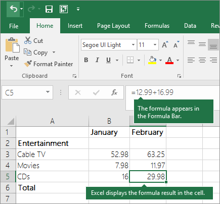
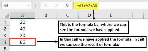
The formula that you enter in a cell remains visible in the formula bar, and you can see it whenever that cell is selected.
Important: Although there is a SUM function, there is no SUBTRACT function. Instead, use the minus (-) operator in a formula; for example, =8-3+2-4+12. Or, you can use a minus sign to convert a number to its negative value in the SUM function; for example, the formula =SUM(12,5,-3,8,-4) uses the SUM function to add 12, 5, subtract 3, add 8, and subtract 4, in that order.
Use AutoSum
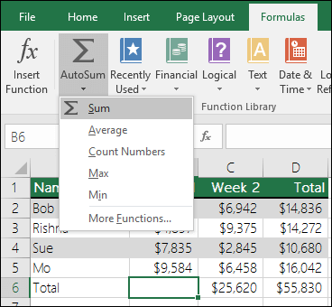
The easiest way to add a SUM formula to your worksheet is to use AutoSum. Select an empty cell directly above or below the range that you want to sum, and on the Home or Formula tabs of the ribbon, click AutoSum > Sum. AutoSum will automatically sense the range to be summed and build the formula for you. This also works horizontally if you select a cell to the left or right of the range that you need to sum.
Note: AutoSum does not work on non-contiguous ranges.
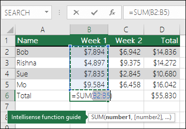
In the figure above, the AutoSum feature is seen to automatically detect cells B2:B5 as the range to sum. All you need to do is press ENTER to confirm it. If you need to add/exclude more cells, you can hold the Shift Key + the arrow key of your choice until your selection matches what you want. Then press Enter to complete the task.
Intellisense function guide: the SUM(number1,[number2], …) floating tag beneath the function is its Intellisense guide. If you click the SUM or function name, it will change o a blue hyperlink to the Help topic for that function. If you click the individual function elements, their representative pieces in the formula will be highlighted. In this case, only B2:B5 would be highlighted, since there is only one number reference in this formula. The Intellisense tag will appear for any function.

Learn more in the article on the SUM function.
Avoid rewriting the same formula
After you create a formula, you can copy it to other cells — no need to rewrite the same formula. You can either copy the formula, or use the fill handle  to copy the formula to adjacent cells.
For example, when you copy the formula in cell B6 to C6, the formula in that cell automatically changes to update to cell references in column C.
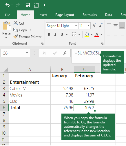
When you copy the formula, ensure that the cell references are correct. Cell references may change if they have relative references. For more information, see Copy and paste a formula to another cell or worksheet.
Источник
Overview of formulas in Excel
Get started on how to create formulas and use built-in functions to perform calculations and solve problems.
Important: The calculated results of formulas and some Excel worksheet functions may differ slightly between a Windows PC using x86 or x86-64 architecture and a Windows RT PC using ARM architecture. Learn more about the differences.
Important: In this article we discuss XLOOKUP and VLOOKUP, which are similar. Try using the new XLOOKUP function, an improved version of VLOOKUP that works in any direction and returns exact matches by default, making it easier and more convenient to use than its predecessor.
Create a formula that refers to values in other cells
Type the equal sign =.
Note: Formulas in Excel always begin with the equal sign.
Select a cell or type its address in the selected cell.

Enter an operator. For example, – for subtraction.
Select the next cell, or type its address in the selected cell.

Press Enter. The result of the calculation appears in the cell with the formula.
See a formula
When a formula is entered into a cell, it also appears in the Formula bar.

To see a formula, select a cell, and it will appear in the formula bar.

Enter a formula that contains a built-in function
Select an empty cell.
Type an equal sign = and then type a function. For example, =SUM for getting the total sales.
Type an opening parenthesis (.
Select the range of cells, and then type a closing parenthesis).

Press Enter to get the result.
Download our Formulas tutorial workbook
We’ve put together a Get started with Formulas workbook that you can download. If you’re new to Excel, or even if you have some experience with it, you can walk through Excel’s most common formulas in this tour. With real-world examples and helpful visuals, you’ll be able to Sum, Count, Average, and Vlookup like a pro.
Formulas in-depth
You can browse through the individual sections below to learn more about specific formula elements.
A formula can also contain any or all of the following: functions, references, operators, and constants.
Parts of a formula
1. Functions: The PI() function returns the value of pi: 3.142.
2. References: A2 returns the value in cell A2.
3. Constants: Numbers or text values entered directly into a formula, such as 2.
4. Operators: The ^ (caret) operator raises a number to a power, and the * (asterisk) operator multiplies numbers.
A constant is a value that is not calculated; it always stays the same. For example, the date 10/9/2008, the number 210, and the text «Quarterly Earnings» are all constants. An expression or a value resulting from an expression is not a constant. If you use constants in a formula instead of references to cells (for example, =30+70+110), the result changes only if you modify the formula. In general, it’s best to place constants in individual cells where they can be easily changed if needed, then reference those cells in formulas.
A reference identifies a cell or a range of cells on a worksheet, and tells Excel where to look for the values or data you want to use in a formula. You can use references to use data contained in different parts of a worksheet in one formula or use the value from one cell in several formulas. You can also refer to cells on other sheets in the same workbook, and to other workbooks. References to cells in other workbooks are called links or external references.
The A1 reference style
By default, Excel uses the A1 reference style, which refers to columns with letters (A through XFD, for a total of 16,384 columns) and refers to rows with numbers (1 through 1,048,576). These letters and numbers are called row and column headings. To refer to a cell, enter the column letter followed by the row number. For example, B2 refers to the cell at the intersection of column B and row 2.
The cell in column A and row 10
The range of cells in column A and rows 10 through 20
The range of cells in row 15 and columns B through E
All cells in row 5
All cells in rows 5 through 10
All cells in column H
All cells in columns H through J
The range of cells in columns A through E and rows 10 through 20
Making a reference to a cell or a range of cells on another worksheet in the same workbook
In the following example, the AVERAGE function calculates the average value for the range B1:B10 on the worksheet named Marketing in the same workbook.
1. Refers to the worksheet named Marketing
2. Refers to the range of cells from B1 to B10
3. The exclamation point (!) Separates the worksheet reference from the cell range reference
Note: If the referenced worksheet has spaces or numbers in it, then you need to add apostrophes (‘) before and after the worksheet name, like =’123′!A1 or =’January Revenue’!A1.
The difference between absolute, relative and mixed references
Relative references A relative cell reference in a formula, such as A1, is based on the relative position of the cell that contains the formula and the cell the reference refers to. If the position of the cell that contains the formula changes, the reference is changed. If you copy or fill the formula across rows or down columns, the reference automatically adjusts. By default, new formulas use relative references. For example, if you copy or fill a relative reference in cell B2 to cell B3, it automatically adjusts from =A1 to =A2.
Copied formula with relative reference
Absolute references An absolute cell reference in a formula, such as $A$1, always refer to a cell in a specific location. If the position of the cell that contains the formula changes, the absolute reference remains the same. If you copy or fill the formula across rows or down columns, the absolute reference does not adjust. By default, new formulas use relative references, so you may need to switch them to absolute references. For example, if you copy or fill an absolute reference in cell B2 to cell B3, it stays the same in both cells: =$A$1.
Copied formula with absolute reference
Mixed references A mixed reference has either an absolute column and relative row, or absolute row and relative column. An absolute column reference takes the form $A1, $B1, and so on. An absolute row reference takes the form A$1, B$1, and so on. If the position of the cell that contains the formula changes, the relative reference is changed, and the absolute reference does not change. If you copy or fill the formula across rows or down columns, the relative reference automatically adjusts, and the absolute reference does not adjust. For example, if you copy or fill a mixed reference from cell A2 to B3, it adjusts from =A$1 to =B$1.
Copied formula with mixed reference
The 3-D reference style
Conveniently referencing multiple worksheets If you want to analyze data in the same cell or range of cells on multiple worksheets within a workbook, use a 3-D reference. A 3-D reference includes the cell or range reference, preceded by a range of worksheet names. Excel uses any worksheets stored between the starting and ending names of the reference. For example, =SUM(Sheet2:Sheet13!B5) adds all the values contained in cell B5 on all the worksheets between and including Sheet 2 and Sheet 13.
You can use 3-D references to refer to cells on other sheets, to define names, and to create formulas by using the following functions: SUM, AVERAGE, AVERAGEA, COUNT, COUNTA, MAX, MAXA, MIN, MINA, PRODUCT, STDEV.P, STDEV.S, STDEVA, STDEVPA, VAR.P, VAR.S, VARA, and VARPA.
3-D references cannot be used in array formulas.
3-D references cannot be used with the intersection operator (a single space) or in formulas that use implicit intersection.
What occurs when you move, copy, insert, or delete worksheets The following examples explain what happens when you move, copy, insert, or delete worksheets that are included in a 3-D reference. The examples use the formula =SUM(Sheet2:Sheet6!A2:A5) to add cells A2 through A5 on worksheets 2 through 6.
Insert or copy If you insert or copy sheets between Sheet2 and Sheet6 (the endpoints in this example), Excel includes all values in cells A2 through A5 from the added sheets in the calculations.
Delete If you delete sheets between Sheet2 and Sheet6, Excel removes their values from the calculation.
Move If you move sheets from between Sheet2 and Sheet6 to a location outside the referenced sheet range, Excel removes their values from the calculation.
Move an endpoint If you move Sheet2 or Sheet6 to another location in the same workbook, Excel adjusts the calculation to accommodate the new range of sheets between them.
Delete an endpoint If you delete Sheet2 or Sheet6, Excel adjusts the calculation to accommodate the range of sheets between them.
The R1C1 reference style
You can also use a reference style where both the rows and the columns on the worksheet are numbered. The R1C1 reference style is useful for computing row and column positions in macros. In the R1C1 style, Excel indicates the location of a cell with an «R» followed by a row number and a «C» followed by a column number.
A relative reference to the cell two rows up and in the same column
A relative reference to the cell two rows down and two columns to the right
An absolute reference to the cell in the second row and in the second column
A relative reference to the entire row above the active cell
An absolute reference to the current row
When you record a macro, Excel records some commands by using the R1C1 reference style. For example, if you record a command, such as clicking the AutoSum button to insert a formula that adds a range of cells, Excel records the formula by using R1C1 style, not A1 style, references.
You can turn the R1C1 reference style on or off by setting or clearing the R1C1 reference style check box under the Working with formulas section in the Formulas category of the Options dialog box. To display this dialog box, click the File tab.
Need more help?
You can always ask an expert in the Excel Tech Community or get support in the Answers community.
Источник
How to Calculate in Excel (Table of Contents)
- Introduction to Calculations in Excel
- Examples of Calculations in Excel
Introduction to Calculations in Excel
The following article provides an outline for Calculations in Excel. MS Excel is the most preferred option for calculation; most investment bankers and financial analysts use it to do data crunching, prepare presentations, or model data.
There are two ways to perform the Excel calculation: Formula and the second is Function. Where formula is the normal arithmetic operation like summation, multiplication, subtraction, etc. Function is the inbuilt formula like SUM (), COUNT (), COUNTA (), COUNTIF (), SQRT () etc.
Operator Precedence: It will use default order to calculate; if there is some operation in parentheses, then it will calculate that part first, then multiplication or division after that addition or subtraction. It is the same as the BODMAS rule.
Examples of Calculations in Excel
Here are some examples of How to Use Excel to Calculate Basic calculations.
You can download this Calculations Excel Template here – Calculations Excel Template
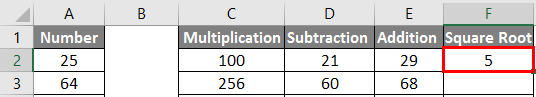
Example #1 – Basic Calculations like Multiplication, Summation, Subtraction, and Square Root
Here we are going to learn how to do basic calculations like multiplication, summation, subtraction, and square root in Excel.
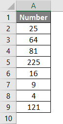
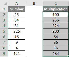
Let’s assume a user wants to perform calculations like multiplication, summation, subtraction by 4 and find out the square root of all numbers in Excel.
Let’s see how we can do this with the help of calculations.
Step 1: Open an Excel sheet. Go to sheet 1 and insert the data as shown below.
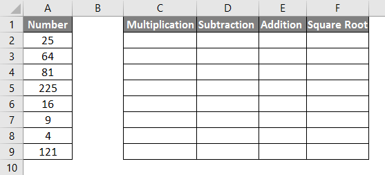
Step 2: Now create headers for Multiplication, Summation, Subtraction, and Square Root in row one.
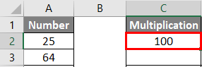
Step 3: Now calculate the multiplication by 4. Use the equal sign to calculate. Write in cell C2 and use asterisk symbol (*) to multiply “=A2*4“

Step 4: Now press on the Enter key; multiplication will be calculated.
Step 5: Drag the same formula to the C9 cell to apply to the remaining cells.
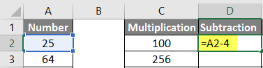
Step 6: Now calculate subtraction by 4. Use an equal sign to calculate. Write in cell D2 “=A2-4“
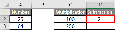
Step 7: Now click on the Enter key, the subtraction will be calculated.
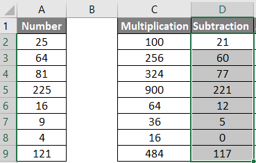
Step 8: Drag the same formula till cell D9 to apply to the remaining cells.
Step 9: Now calculate the addition by 4, use an equal sign to calculate. Write in E2 Cell “=A2+4“
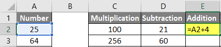
Step 10: Now press on the Enter key, the addition will be calculated.
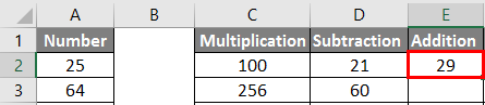
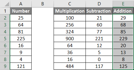
Step 11: Drag the same formula to the E9 cell to apply to the remaining cells.
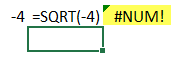
Step 12: Now calculate the square root>> use equal sign to calculate >> Write in F2 Cell >> “=SQRT (A2“
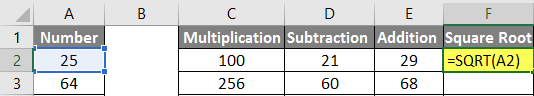
Step 13: Now, press on the Enter key >> square root will be calculated.
Step 14: Drag the same formula till the F9 cell to apply the remaining cell.
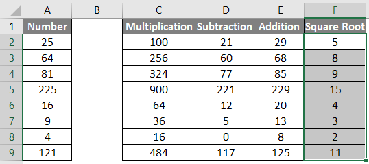
Summary of Example 1: As the user wants to perform calculations like multiplication, summation, subtraction by 4 and find out the square root of all numbers in MS Excel.
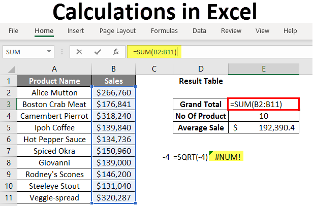
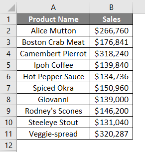
Example #2 – Basic Calculations like Summation, Average, and Counting
Here we are going to learn how to use Excel to calculate basic calculations like summation, average, and counting.
Let’s assume a user wants to find out total sales, average sales, and the total number of products available in his stock for sale.
Let’s see how we can do this with the help of calculations.
Step 1: Open an Excel sheet. Go to Sheet1 and insert the data as shown below.
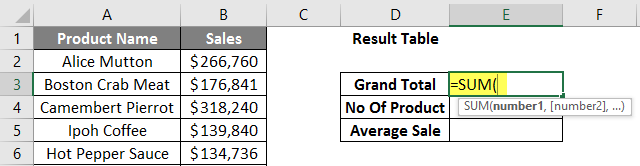
Step 2: Now create headers for Result table, Grand Total, Number of Product and an Average Sale of his product in column D.
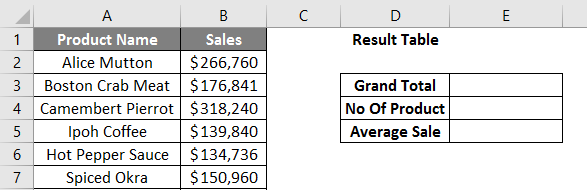
Step 3: Now calculate grand total sales. Use the SUM function to calculate the grand total. Write in cell E3. “=SUM (“
Step 4: Now, it will ask for the numbers, so give the data range, which is available in column B. Write in cell E3. “=SUM (B2:B11) “
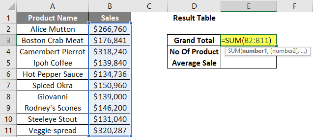
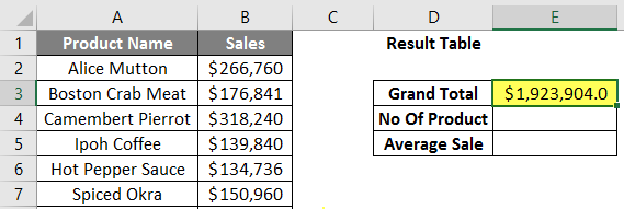
Step 5: Now press on the Enter key. Grand total sales will be calculated.
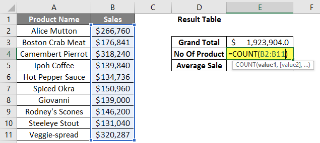
Step 6: Now calculate the total number of products in the stock, use the COUNT function to calculate the grand total. Write in cell E4 “=COUNT (“
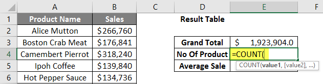
Step 7: Now, it will ask for the values, so give the data range, which is available in column B. Write in cell E4. “=COUNT (B2:B11) “
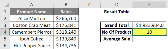
Step 8: Now press on the Enter key. The total number of products will be calculated.
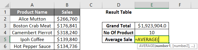
Step 9: Now calculate the average sale of products in the stock, use the AVERAGE function to calculate the average sale. Write in cell E5. “=AVERAGE (“
Step 10: Now, it will ask for the numbers, so give the data range which is available in column B. Write in cell E5. “=AVERAGE (B2:B11) “
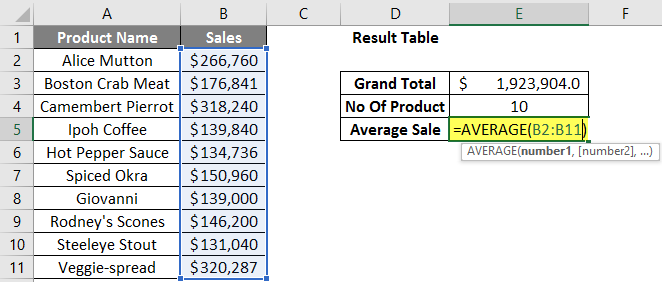
Step 11: Now click on the Enter key. The average sale of products will be calculated.
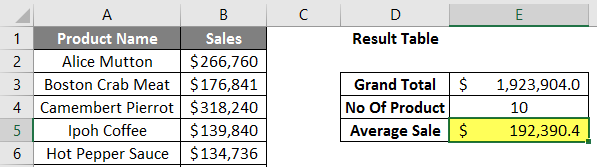
Summary of Example 2: As the user wants to find out total sales, average sales, and the total number of products available in his stock for sale.
Things to Remember about Calculations in Excel
- During calculations, if there are some operations in parentheses, then it will calculate that part first, then multiplication or division after that addition or subtraction.
- It is the same as the BODMAS rule: Parentheses, Exponents, Multiplication and Division, Addition and Subtraction.
- When a user uses an equal sign (=) in any cell, it means that the user is going to put some formula, not a value.
- A small difference from the normal mathematics symbol like multiplication uses asterisk symbol (*) and for division uses forward-slash (/).
- There is no need to write the same formula for each cell; once it is written, then just copy-paste to other cells, it will calculate automatically.
- A user can use the SQRT function to calculate the square root of any value; it has only one parameter. But a user cannot calculate square root for a negative number; it will throw an error #NUM!
- If a negative value occurs as output, use the ABS formula to determine the absolute value, which is an in-built function in MS Excel.
- A user can use the COUNTA in-built function if there is confusion in the data type because COUNT supports only numeric values.
Recommended Articles
This is a guide to Calculations in Excel. Here we discuss how to use excel to calculate along with examples and a downloadable excel template. You may also look at the following articles to learn more –
- Create a Lookup Table in Excel
- Use of COLUMNS Formula in Excel
- CHOOSE Formula in Excel with Examples
- What is Chart Wizard in Excel?
How to Use Excel as a Calculator?
In Excel, by default, there is no calculator button or option available in it. But, we can enable it manually from the “Options” section and then from the “Quick Access Toolbar,” where we can go to the commands not available in the ribbon. There further, we will find the calculator option available. Just click on “Add” and the “OK” to add the calculator to our Excel ribbon.
I have never seen beyond Excel to do the calculations in my career. Most of the calculations are possible with Excel spreadsheets. Not only are the calculations, but they are also flexible enough to reflect the immediate results if there are any modifications to the numbers, which is the power of applying formulas.
By using formulas, we need to worry about all the steps in the calculations because formulas will capture the numbers and show immediate real-time results for us. Excel has hundreds of built-in formulas to work with some of the complex calculations. On top of this, we see the spreadsheet as a mathematics calculator to add, divide, subtract, and multiply.
Table of contents
- How to Use Excel as a Calculator?
- How to Calculate in Excel Sheet?
- Example #1 – Use Formulas in Excel as a Calculator
- Example #2 – Use Cell References
- Example #3 – Cell Reference Formulas are Flexible
- Example #4 – Formula Cell is not Value, It is the only Formula
- Example #5 – Built-In Formulas are Best Suited for Excel
- Recommended Articles
- How to Calculate in Excel Sheet?
This article will show you how to use Excel as a calculator.
How to Calculate in Excel Sheet?
Below are examples of how to use Excel as a calculator.
You can download this Calculation in Excel Template here – Calculation in Excel Template
Example #1 – Use Formulas in Excel as a Calculator
As told, Excel has many of its built-in formulas, and on top of this, we can use Excel in the form of a calculator. To enter anything in the cell, we type the content in the required cell but apply the formula, and we need to start the equal sign in the cell.
Follow the below steps.
- So, to start any calculation, we need first to enter an equal sign, indicating that we are not just entering. Rather, we are entering the formula.

- Once the equal sign is entered in the cell, we can enter the formula. For example, assume that if we want to calculate the addition of two numbers, 50 and 30, we first need to enter the number we want to add.

- Once the number is entered, we need to go back to the basics of mathematics. Since we are doing the addition, we need to apply the PLUS (+) sign.

- After the addition sign (+), we must enter the second number. Then, we need to add to the first number.

- Now, press the ENTER key to get the result in cell A1.


So, 50 + 30 = 80.
It is the basic use of ExcelIn today’s corporate working and data management process, Microsoft Excel is a powerful tool.» Every employee is required to have this expertise. The primary uses of Excel are as follows: Data Analysis and Interpretation, Data Organizing and Restructuring, Data Filtering, Goal Seek Analysis, Interactive Charts and Graphs.
read more as a calculator. Similarly, we can use cell references to the formulaCell reference in excel is referring the other cells to a cell to use its values or properties. For instance, if we have data in cell A2 and want to use that in cell A1, use =A2 in cell A1, and this will copy the A2 value in A1.read more.
Example #2 – Use Cell References
For example, look at the below values in cells A1, A2, and A3.

- We must open an equal sign in the A4 cell.

- Then, select cell A1 first.

- After selecting cell A1, we need to put a plus sign and choose the A2 cell.

- Now, put one more plus sign and select A3 cell.
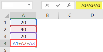
- Press the “ENTER” key to get the result in the A4 cell.
It is the result of using cell references.
Example #3 – Cell Reference Formulas are Flexible
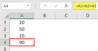
By using cell references, we can make the formula real-time and flexible. We said cell reference formulas are flexible because if we make any changes to the formula input cells (A1, A2, A3), it will reflect the changes in the formula cell (A4).
- We will change the number in cell A2 from 40 to 50.

We have changed the number but have not yet pressed the “ENTER” key. If we hit the “ENTER” key, we can see the result in the A4 cell.
- The moment we press the “ENTER” key, we see the impact on cell A4.
Example #4 – Formula Cell is not Value, It is the only Formula
We need to know when we use a cell reference for formulas because formula cells hold the result of the formula, not the value itself.
- Suppose we have a value of 50 in cell C2.

- If we copy and paste it to the next cell, we still get the value of 50 only.

- But, now come back to cell A4.

- Here we can see 90, but this is not the value but the formula. So we will copy and paste it to the next cell and see what we get.

Oh oh!!! We got zero.
We got zero because cell A4 has the formula =A1 + A2 + A3. When we copy cell A4 and paste it to B4, formula-referenced cells are changed from A1 + A2 + A3 to B1 + B2 + B3.
We got zero since there are no values in the cells B1, B2, and B3. So now, we will put 60 in any of the cells in B1, B2, and B3 and see the result.

- Look here the moment we have entered 60; we got the result as 60 because cell B4 already has the cell reference of the above three cells (B1, B2, and B3).

Example #5 – Built-In Formulas are Best Suited for Excel
We have seen how to use cell references for the formulas in the above examples. But those are best suited only for the small number of data sets, for a maximum of 5 to 10 cells.
Now, look at the below data.

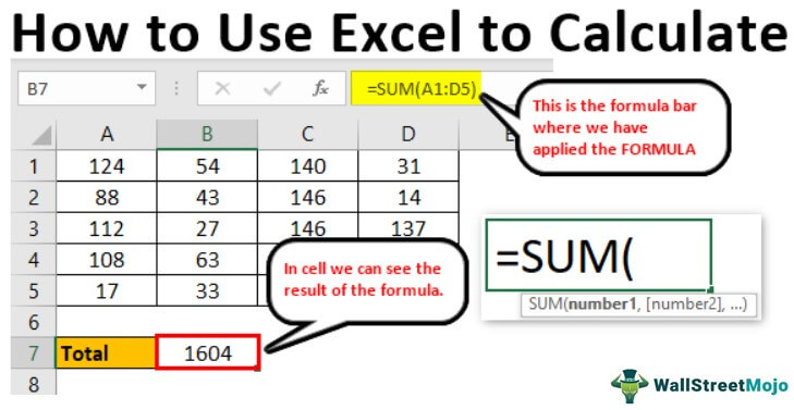
We have numbers from A1 to D5, and in the B7 cell, we need the total of these numbers. In these large data sets, we cannot give individual cell references, which takes a lot of time for us. That is where Excel’s built-in formulas come into the example.
- We should first open the SUM functionThe SUM function in excel adds the numerical values in a range of cells. Being categorized under the Math and Trigonometry function, it is entered by typing “=SUM” followed by the values to be summed. The values supplied to the function can be numbers, cell references or ranges.read more in cell B7.

- Now, hold the left-click of the mouse and select the range of cells from A1 to D5.

- After that, close the bracket and press the “Enter” key.

So, like this, we can use built-in formulas to work with large data sets.
This way, we can calculate in the Excel sheet.
Recommended Articles
This article is a guide to Excel as a Calculator. Here, we discuss how to do a calculation in an Excel sheet with examples and downloadable Excel templates. You may also look at these useful functions in Excel: –
- Calculate Percentage in Excel Formula
- Multiply in Excel Formula
- How to Divide using Excel Formulas?
- Excel Subtraction Formula
If you’re getting started with Excel, creating formulas is one of the first things you should learn. In this lesson you’ll learn how to create simple formulas and calculations in Excel.
At its heart, Excel is a giant calculator. In fact, a simple way to think about Excel is to consider each cell in a worksheet like an individual calculator. An Excel spreadsheet has millions of cells, which means you have millions of individual calculators to work with. Not only that, but you can create formulas that link different cells together (e.g. add the value in this cell to the value in that cell). You can create formulas that link cells in different worksheets together. And you can even create formulas that link cells in different workbooks together.
How to enter a formula in Excel
In Excel, each cell can contain a calculation. In Excel jargon we call this a formula. Each cell can contain one formula. When you enter a formula in a cell, Excel calculates the result of that formula and displays the result of that calculation to you. In fact, when you enter a formula into any cell, Excel will recalculate the result of all the cells in the worksheet. This normally happens in the blink of an eye so you won’t normally notice it, although you may find that large and complex spreadsheets can take longer to recalculate.
When entering a formula, you have to make sure Excel knows that’s what you want to do. You start by typing the = (equals) sign, then the rest of your formula. If you don’t type the equals sign first, then Excel will assume you are typing either a number or a text. You can also start a formula with either a plus (+) or minus (-) symbol. Excel will assume you’re typing a formula and insert the equals sign for you.
Here are some examples of some simple Excel formulas and their results:
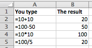
In this example, there are four basic formulas:
- Addition (+)
- Subtraction (—)
- Multiplication (*)
- Division (/)
In each case, you would type the equals sign (=), then the formula, then press Enter to tell Excel you’ve finished.
- Sometimes Excel will show you a warning rather than just entering your formula. This will happen if the formula you’ve typed is invalid, i.e. is not in a format that Excel recognises. It will usually also give you some indication of what you did wrong.
- Other times, Excel may enter the formula you have typed correctly but then show you an error such as #VALUE. This means that you have entered a formula that was value, but Excel could not calculate a valid result from your formula.
Creating formulas that refer to other cells in the same worksheet
Excel’s power comes from allowing you to create formulas that refer to the values in other cells.
In the example above, you’ll notice the headings across the top (A, B) and down the left (1,2,3,4,5). By comining these values, we have a unique reference each cell in a worksheet (A1, A2, A3, B1, B2, B3, and so on).
When you create a formula, you can refer to other cells using these cell references to incorporate the values in other cells into a formula. The value in another cell might be a simple number, or another cell containing a formula. When you create a formula that refers to another cell that also contains a formula, your formula will use the result of the formula in that other cell. Then, if the result of the formula in that other cell changes, so too does the result in your formula.
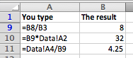
Here are some examples of some Excel formulas that refer to other cells:
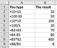
In this example, rows 6-8 build on the earlier examples to link cells together:
- B6 adds the values in B2 and B3 together. If you change either of the values in B2 or B3 the result in B6 will change too.
- B7 and B8 subtract and multiply the values in other cells.
- B9 goes a step further and divides B8 by B3. Note that B8 in turn multiplied B5 and B2 together. So changing the values in either B5 or B2 will have a domino effect, where the value in B8 will change, and so the value in B9 will change too. Note that Excel handles all of this the moment you finish entering a change in either B5 or B2.
Creating formulas that refer to cells in other worksheets
When you first open Excel, you start with a single worksheet. However, Excel allows you to have more than one worksheet inside a single spreadsheet file (known as a workbook). In fact, in earlier versions of Excel a new workbook automatically started out with 3 worksheets inside it.
Earlier we saw how to link two cells together within a worksheet by referring to other cells using their cell reference value. Referring to a cell inside another worksheet works in much the same way, but we need to provide more information about the location of that cell so Excel knows which cell we’re talking about.
Here are some examples of formulas that refer to cells in another worksheet inside the same workbook:
In this example, the formulas in B10 and B11 refer to cells in another worksheet called Data.
- B10 multiples the value in B9 by the value in cell A2 in the worksheet called Data
- B11 takes the value A4 in the worksheet called Data and divides it by the value in B9.
In other words, we’ve told Excel to go to the worksheet called Data and use values in that worksheet in our formulas.
There are a couple of ways to create formulas like this:
- Type the formula in by hand. In the above example, you would create the reference to the other worksheet by typing the worksheet name followed by an exclamation mark (!); the exclamation mark tells Excel that you’re referring to another worksheet.
- Start typing the formula by typing the equals sign (=), then click on the name of the other worksheet. Excel will switch to the other worksheet, and you can click on the cell you want to reference in your formula. You can then press Enter to finish entering the formula, or you can click back on the original worksheet name and finish typing your formula before pressing Enter.
Note that if you rename the worksheet called Data, the formulas that refer to Data will automatically update to reflect the new name. Here’s what the above examples look like if we change the name of the worksheet called Data to Daily Data.
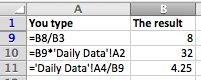
Note how Excel has put apostrophes around the name of the worksheet called Daily Data. This is because of the space in the worksheet name. Excel does this to make sure that the reference still works; if you manually type the formula without the apostrophes then Excel will not be able to validate the formula, and will not let you enter it.
Creating formulas that link to other workbooks
As you might imagine what we’ve already covered, it is also possible to create a formulat that refers to cells in another workbook (i.e. another file). Once again, it’s simply a matter of correctly referring to the cell in the other workbook.
The following example shows what this looks like:
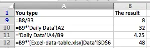
In this example, B12 contains a formula that refers to cell D6 in a worksheet called Data in a file called Excel-data-table-xlsx.
- The square brackets are used to indicate the filename, i.e. [filename]. Be aware that if the file referred to is not currently open, the square brackets may also include the full file path to that file, so that Excel can still read the value from the cell being referred to even though the file is not open.
- The apostrophes are used to enclose the full file name and worksheet name.
- Then, Excel uses absolute references to identify the cell being referred to. This means that if you move (not copy) the contents of cell D6 in the Data worksheet, your formula will still work. The $ signs are used to denote an absolute reference (as opposed to a relative reference). Absolute and relative references are out of scope for this lesson, but you can read about them in this lesson.
Summary
Learning to use Excel formulas is one of the most important things you’ll learn to do with Excel. Hopefully this lesson has set you on the right path, and you’ll be creating spreadsheets with formulas of your own in no time at all. If you have any feedback or questions on this lesson, please comment below!
.