
Excel for Microsoft 365 Excel for Microsoft 365 for Mac Excel for the web Excel 2021 Excel 2021 for Mac Excel 2019 Excel 2019 for Mac Excel 2016 Excel 2016 for Mac Excel 2013 Excel 2010 Excel 2007 Excel for Mac 2011 Excel Starter 2010 More…Less
This article describes the formula syntax and usage of the AVERAGE function in Microsoft Excel.
Description
Returns the average (arithmetic mean) of the arguments. For example, if the range A1:A20 contains numbers, the formula =AVERAGE(A1:A20) returns the average of those numbers.
Syntax
AVERAGE(number1, [number2], …)
The AVERAGE function syntax has the following arguments:
-
Number1 Required. The first number, cell reference, or range for which you want the average.
-
Number2, … Optional. Additional numbers, cell references or ranges for which you want the average, up to a maximum of 255.
Remarks
-
Arguments can either be numbers or names, ranges, or cell references that contain numbers.
-
Logical values and text representations of numbers that you type directly into the list of arguments are not counted.
-
If a range or cell reference argument contains text, logical values, or empty cells, those values are ignored; however, cells with the value zero are included.
-
Arguments that are error values or text that cannot be translated into numbers cause errors.
-
If you want to include logical values and text representations of numbers in a reference as part of the calculation, use the AVERAGEA function.
-
If you want to calculate the average of only the values that meet certain criteria, use the AVERAGEIF function or the AVERAGEIFS function.
Note: The AVERAGE function measures central tendency, which is the location of the center of a group of numbers in a statistical distribution. The three most common measures of central tendency are:
-
Average, which is the arithmetic mean, and is calculated by adding a group of numbers and then dividing by the count of those numbers. For example, the average of 2, 3, 3, 5, 7, and 10 is 30 divided by 6, which is 5.
-
Median, which is the middle number of a group of numbers; that is, half the numbers have values that are greater than the median, and half the numbers have values that are less than the median. For example, the median of 2, 3, 3, 5, 7, and 10 is 4.
-
Mode, which is the most frequently occurring number in a group of numbers. For example, the mode of 2, 3, 3, 5, 7, and 10 is 3.
For a symmetrical distribution of a group of numbers, these three measures of central tendency are all the same. For a skewed distribution of a group of numbers, they can be different.
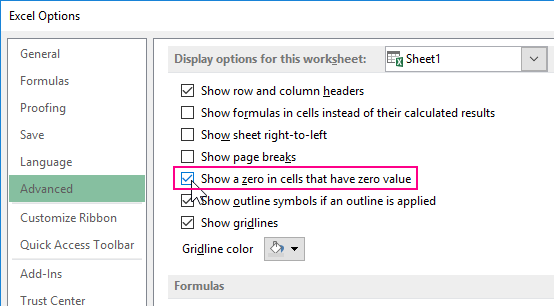
Tip: When you average cells, keep in mind the difference between empty cells and those containing the value zero, especially if you have cleared the Show a zero in cells that have a zero value check box in the Excel Options dialog box in the Excel desktop application. When this option is selected, empty cells are not counted, but zero values are.
To locate the Show a zero in cells that have a zero value check box:
-
On the File tab, click Options, and then, in the Advanced category, look under Display options for this worksheet.
Example
Copy the example data in the following table, and paste it in cell A1 of a new Excel worksheet. For formulas to show results, select them, press F2, and then press Enter. If you need to, you can adjust the column widths to see all the data.
|
Data |
||
|
10 |
15 |
32 |
|
7 |
||
|
9 |
||
|
27 |
||
|
2 |
||
|
Formula |
Description |
Result |
|
=AVERAGE(A2:A6) |
Average of the numbers in cells A2 through A6. |
11 |
|
=AVERAGE(A2:A6, 5) |
Average of the numbers in cells A2 through A6 and the number 5. |
10 |
|
=AVERAGE(A2:C2) |
Average of the numbers in cells A2 through C2. |
19 |
Need more help?
![]()
Download Article
![]()
Download Article
Mathematically speaking, “average” is used by most people to mean “central tendency,” which refers to the centermost of a range of numbers. There are three common measures of central tendency: the (arithmetic) mean, the median, and the mode. Microsoft Excel has functions for all three measures, as well as the ability to determine a weighted average, which is useful for finding an average price when dealing with different quantities of items with different prices.
-

1
Enter the numbers you want to find the average of. To illustrate how each of the central tendency functions works, we’ll use a series of ten small numbers. (You won’t likely use actual numbers this small when you use the functions outside these examples.)
- Most of the time, you’ll enter numbers in columns, so for these examples, enter the numbers in cells A1 through A10 of the worksheet.
- The numbers to enter are 2, 3, 5, 5, 7, 7, 7, 9, 16, and 19.
- Although it isn’t necessary to do this, you can find the sum of the numbers by entering the formula “=SUM(A1:A10)” in cell A11. (Don’t include the quotation marks; they’re there to set off the formula from the rest of the text.)
-
2
Find the average of the numbers you entered. You do this by using the AVERAGE function. You can place the function in one of three ways:
- Click on an empty cell, such as A12, then type “=AVERAGE(A1:10)” (again, without the quotation marks) directly in the cell.
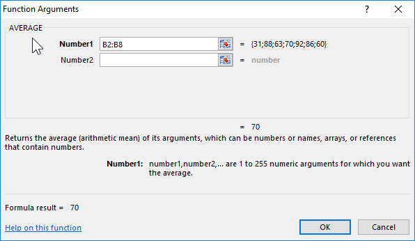
- Click on an empty cell, then click on the “fx” symbol in the function bar above the worksheet. Select “AVERAGE” from the “Select a function:” list in the Insert Function dialog and click OK. Enter the range “A1:A10” in the Number 1 field of the Function Arguments dialog and click OK.
- Enter an equals sign (=) in the function bar to the right of the function symbol. Select the AVERAGE function from the Name box dropdown list to the left of the function symbol. Enter the range “A1:A10” in the Number 1 field of the Function Arguments dialog and click OK.
Advertisement
-
3
Observe the result in the cell you entered the formula in. The average, or arithmetic mean, is determined by finding the sum of the numbers in the cell range (80) and then dividing the sum by how many numbers make up the range (10), or 80 / 10 = 8.
- If you calculated the sum as suggested, you can verify this by entering “=A11/10” in any empty cell.
- The mean value is considered a good indicator of central tendency when the individual values in the sample range are fairly close together. It is not considered as good of an indicator in samples where there are a few values that differ widely from most of the other values.


Advertisement
-
1
Enter the numbers you want to find the median for. We’ll use the same range of ten numbers (2, 3, 5, 5, 7, 7, 7, 9, 16, and 19) as we used in the method for finding the mean value. Enter them in the cells from A1 to A10, if you haven’t already done so.
-
2
Find the median value of the numbers you entered. You do this by using the MEDIAN function. As with the AVERAGE function, you can enter it one of three ways:
- Click on an empty cell, such as A13, then type “=MEDIAN(A1:10)” (again, without the quotation marks) directly in the cell.
- Click on an empty cell, then click on the “fx” symbol in the function bar above the worksheet. Select “MEDIAN” from the “Select a function:” list in the Insert Function dialog and click OK. Enter the range “A1:A10” in the Number 1 field of the Function Arguments dialog and click OK.
- Enter an equals sign (=) in the function bar to the right of the function symbol. Select the MEDIAN function from the Name box dropdown list to the left of the function symbol. Enter the range “A1:A10” in the Number 1 field of the Function Arguments dialog and click OK.
-
3
Observe the result in the cell you entered the function in. The median is the point where half the numbers in the sample have values higher than the median value and the other half have values lower than the median value. (In the case of our sample range, the median value is 7.) The median may be the same as one of the values in the sample range, or it may not.


Advertisement
-
1
Enter the numbers you want to find the mode for. We’ll use the same range of numbers (2, 3, 5, 5, 7, 7, 7, 9, 16, and 19) again, entered in cells from A1 through A10.
-
2
Find the mode value for the numbers you entered. Excel has different mode functions available, depending on which version of Excel you have.
- For Excel 2007 and earlier, there is a single MODE function. This function will find a single mode in a sample range of numbers.
- For Excel 2010 and later, you can use either the MODE function, which works the same as in earlier versions of Excel, or the MODE.SNGL function, which uses a supposedly more accurate algorithm to find the mode.[1]
(Another mode function, MODE.MULT returns multiple values if it finds multiple modes in a sample, but it is intended for use with arrays of numbers instead of a single list of values.[2]
)
-
3
Enter the mode function you’ve chosen. As with the AVERAGE and MEDIAN functions, there are three ways to do this:
- Click on an empty cell, such as A14 then type “=MODE(A1:10)” (again, without the quotation marks) directly in the cell. (If you wish to use the MODE.SNGL function, type “MODE.SNGL” in place of “MODE” in the equation.)
- Click on an empty cell, then click on the “fx” symbol in the function bar above the worksheet. Select “MODE” or “MODE.SNGL,” from the “Select a function:” list in the Insert Function dialog and click OK. Enter the range “A1:A10” in the Number 1 field of the Function Arguments dialog and click OK.
- Enter an equals sign (=) in the function bar to the right of the function symbol. Select the MODE or MODE.SNGL function from the Name box dropdown list to the left of the function symbol. Enter the range “A1:A10” in the Number 1 field of the Function Arguments dialog and click OK.
-
4
Observe the result in the cell you entered the function in. The mode is the value that occurs most often in the sample range. In the case of our sample range, the mode is 7, as 7 occurs three times in the list.
- If two numbers appear in the list the same number of times, the MODE or MODE.SNGL function will report the value that it encounters first. If you change the “3” in the sample list to a “5,” the mode will change from 7 to 5, because the 5 is encountered first. If, however, you change the list to have three 7s before three 5s, the mode will again be 7.


Advertisement
-
1
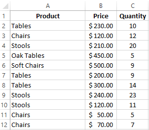
Enter the data you want to calculate a weighted average for. Unlike finding a single average, where we used a one-column list of numbers, to find a weighted average we need two sets of numbers. For the purpose of this example, we’ll assume the items are shipments of tonic, dealing with a number of cases and the price per case.
- For this example, we’ll include column labels. Enter the label “Price Per Case” in cell A1 and “Number of Cases” in cell B1.
- The first shipment was for 10 cases at $20 per case. Enter “$20” in cell A2 and “10” in cell B2.
- Demand for tonic increased, so the second shipment was for 40 cases. However, due to demand, the price of tonic went up to $30 per case. Enter “$30” in cell A3 and “40” in cell B3.
- Because the price went up, demand for tonic went down, so the third shipment was for only 20 cases. With the lower demand, the price per case went down to $25. Enter “$25” in cell A4 and “20” in cell B4.
-
2
Enter the formula you need to calculate the weighted average. Unlike figuring a single average, Excel doesn’t have a single function to figure a weighted average. Instead you’ll use two functions:
- SUMPRODUCT. The SUMPRODUCT function multiplies the numbers in each row together and adds them to the product of the numbers in each of the other rows. You specify the range of each column; since the values are in cells A2 to A4 and B2 to B4, you’d write this as “=SUMPRODUCT(A2:A4,B2:B4)”. The result is the total dollar value of all three shipments.
- SUM. The SUM function adds the numbers in a single row or column. Because we want to find an average for the price of a case of tonic, we’ll sum up the number of cases that were sold in all three shipments. If you wrote this part of the formula separately, it would read “=SUM(B2:B4)”.
-
3
Since an average is determined by dividing a sum of all numbers by the number of numbers, we can combine the two functions into a single formula, written as “=SUMPRODUCT(A2:A4,B2:B4)/ SUM(B2:B4)”.
-
4
Observe the result in the cell you entered the formula in. The average per-case price is the total value of the shipment divided by the total number of cases that were sold.
- The total value of the shipments is 20 x 10 + 30 x 40 + 25 x 20, or 200 + 1200 + 500, or $1900.
- The total number of cases sold is 10 + 40 + 20, or 70.
- The average per case price is 1900 / 70 = $27.14.


Advertisement
Ask a Question
200 characters left
Include your email address to get a message when this question is answered.
Submit
Advertisement
wikiHow Video: How to Calculate Averages in Excel
-
You do not have to enter all the numbers in a continuous column or row, but you do have to make sure Excel understands which numbers you want to include and exclude. If you only wanted to average the first five numbers in our examples on mean, median, and mode and the last number, you’d enter the formula as “=AVERAGE(A1:A5,A10)”.
Thanks for submitting a tip for review!
Advertisement
References
About This Article
Article SummaryX
To calculate averages in Excel, start by clicking on an empty cell. Then, type =AVERAGE followed by the range of cells you want to find the average of in parenthesis, like =AVERAGE(A1:A10). This will calculate the average of all of the numbers in that range of cells. It’s as easy as that! For step-by-step instructions with pictures, check out the full article below!
Did this summary help you?
Thanks to all authors for creating a page that has been read 185,197 times.
Is this article up to date?
Содержание
- AVERAGE function
- Description
- Syntax
- Remarks
- Example
- Calculate the average of a group of numbers
- Average a group of numbers
- Want more?
- How to find the arithmetic mean in Excel?
- How to find the arithmetic mean?
- Average value by condition
- How to calculate the weighted average price in Excel?
- The standard deviation: the formula in Excel
- AVERAGE Function
- Related functions
- Summary
- Purpose
- Return value
- Arguments
- Syntax
- Usage notes
- Basic usage
- Blank cells
- Mixed arguments
- Average with criteria
- Average top 3
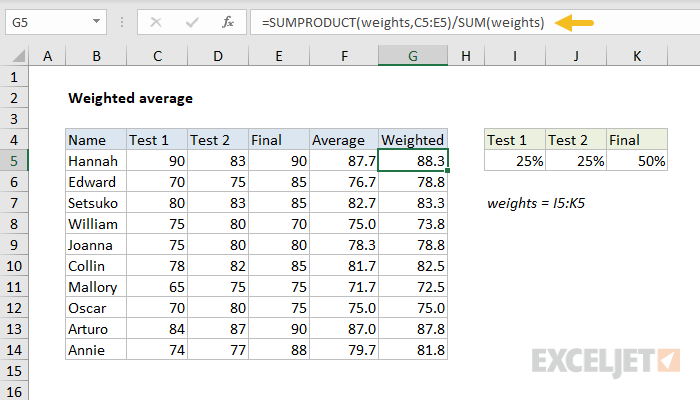
- Weighted average
- Average without #DIV/0!
- Manual average
AVERAGE function
This article describes the formula syntax and usage of the AVERAGE function in Microsoft Excel.
Description
Returns the average (arithmetic mean) of the arguments. For example, if the range A1:A20 contains numbers, the formula = AVERAGE( A1:A20) returns the average of those numbers.
Syntax
The AVERAGE function syntax has the following arguments:
Number1 Required. The first number, cell reference, or range for which you want the average.
Number2, . Optional. Additional numbers, cell references or ranges for which you want the average, up to a maximum of 255.
Arguments can either be numbers or names, ranges, or cell references that contain numbers.
Logical values and text representations of numbers that you type directly into the list of arguments are not counted.
If a range or cell reference argument contains text, logical values, or empty cells, those values are ignored; however, cells with the value zero are included.
Arguments that are error values or text that cannot be translated into numbers cause errors.
If you want to include logical values and text representations of numbers in a reference as part of the calculation, use the AVERAGEA function.
If you want to calculate the average of only the values that meet certain criteria, use the AVERAGEIF function or the AVERAGEIFS function.
Note: The AVERAGE function measures central tendency, which is the location of the center of a group of numbers in a statistical distribution. The three most common measures of central tendency are:
Average, which is the arithmetic mean, and is calculated by adding a group of numbers and then dividing by the count of those numbers. For example, the average of 2, 3, 3, 5, 7, and 10 is 30 divided by 6, which is 5.
Median, which is the middle number of a group of numbers; that is, half the numbers have values that are greater than the median, and half the numbers have values that are less than the median. For example, the median of 2, 3, 3, 5, 7, and 10 is 4.
Mode, which is the most frequently occurring number in a group of numbers. For example, the mode of 2, 3, 3, 5, 7, and 10 is 3.
For a symmetrical distribution of a group of numbers, these three measures of central tendency are all the same. For a skewed distribution of a group of numbers, they can be different.
Tip: When you average cells, keep in mind the difference between empty cells and those containing the value zero, especially if you have cleared the Show a zero in cells that have a zero value check box in the Excel Options dialog box in the Excel desktop application. When this option is selected, empty cells are not counted, but zero values are.
To locate the Show a zero in cells that have a zero value check box:
On the File tab, click Options, and then, in the Advanced category, look under Display options for this worksheet.
Example
Copy the example data in the following table, and paste it in cell A1 of a new Excel worksheet. For formulas to show results, select them, press F2, and then press Enter. If you need to, you can adjust the column widths to see all the data.
Источник
Calculate the average of a group of numbers
Let’s say you want to find the average number of days to complete a tasks by different employees. Or, you want to calculate the average temperature on a particular day over a 10-year time span. There are several ways to calculate the average of a group of numbers.
The AVERAGE function measures central tendency, which is the location of the center of a group of numbers in a statistical distribution. The three most common measures of central tendency are:
Average This is the arithmetic mean, and is calculated by adding a group of numbers and then dividing by the count of those numbers. For example, the average of 2, 3, 3, 5, 7, and 10 is 30 divided by 6, which is 5.
Median The middle number of a group of numbers. Half the numbers have values that are greater than the median, and half the numbers have values that are less than the median. For example, the median of 2, 3, 3, 5, 7, and 10 is 4.
Mode The most frequently occurring number in a group of numbers. For example, the mode of 2, 3, 3, 5, 7, and 10 is 3.
For a symmetrical distribution of a group of numbers, these three measures of central tendency are all the same. In a skewed distribution of a group of numbers, they can be different.
Do the following:
Click a cell below, or to the right, of the numbers for which you want to find the average.
On the Home tab, in the Editing group, click the arrow next to  AutoSum , click Average, and then press Enter.
To do this task, use the AVERAGE function. Copy the table below to a blank worksheet.
Averages all of numbers in list above (9.5)
Averages the top three and the last number in the list (7.5)
Averages the numbers in the list except those that contain zero, such as cell A6 (11.4)
To do this task, use the SUMPRODUCT and SUM functions. vThis example calculates the average price paid for a unit across three purchases, where each purchase is for a different number of units at a different price per unit.
Источник
Average a group of numbers

You may have used AutoSum to quickly add numbers in Excel. But did you know you can also use it to calculate other results, such as averages?
Use AutoSum to quickly find the average
AutoSum lets you find the average in a column or row of numbers where there are no blank cells.
Click a cell below the column or to the right of the row of the numbers for which you want to find the average.
On the HOME tab, click the arrow next to AutoSum > Average, and then press Enter.
Want more?
You may have used AutoSum to quickly add numbers in Excel.
But did you know you can also use it to calculate other results, such as averages?
Click the cell to the right of a row or below a column. Then, on the HOME tab, click the AutoSum down arrow, click Average, verify the formula if what you want, and press Enter.
When I double-click inside the cell, I see it is a formula with the AVERAGE function.
The formula is AVERAGE, A2, colon, A5, which averages the cells from A2 through A5.
When averaging a few cells, the AVERAGE function saves your time. With larger ranges of cells, it’s essential.
If I try to use the AutoSum, Average option here, it only uses cell C5, not the entire column.
Why? Because C4 is blank.
If C4 contained a number, C2 through C5 would be an adjacent range of cells that AutoSum would recognize.
To average values in cells and ranges of cells that aren’t adjacent, type an equals sign (a formula always starts with an equals sign), AVERAGE, open parenthesis, hold down the Ctrl key, click the desired cells and ranges of cells, and press Enter.
The formula uses the AVERAGE function to average the cells containing numbers and ignores the empty cells or those containing text.
For more information about the AVERAGE function, see the course summary at the end of the course.
Источник
How to find the arithmetic mean in Excel?
There are many functions in order to find the average in Excel (although it does not matter what kind of value it is: numerical, textual, percentage or other). And each of them has its own peculiarities and advantages. After all, certain conditions can be put in this task.
For example, the average in Excel is counting using statistical functions. You can also manually enter your own formula. Consider the various options.
How to find the arithmetic mean?
It is necessary to add all the numbers in the set and divide the sum by the number in order to find the arithmetic mean. For example, the student’s marks in computer science: 3, 4, 3, 5, 5. The average rating is 4 for a quarter. We found the arithmetic mean using the formula: =(3 + 4 + 3 + 5 + 5) / 5.
How can you quickly do this with Excel functions? Take for example a number of random numbers in a row:

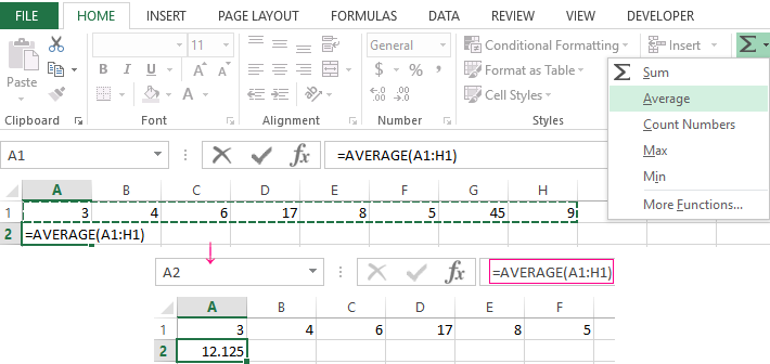
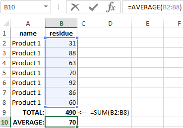
- We put the cursor in cell A2 (under a set of numbers). In the menu – «HOME»-«Editing»-«AutoSum»-«Average» button. A formula appears after clicking in the active cell. Select the range: A1: H1 and press ENTER.
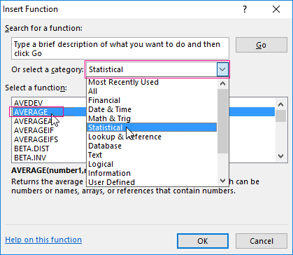
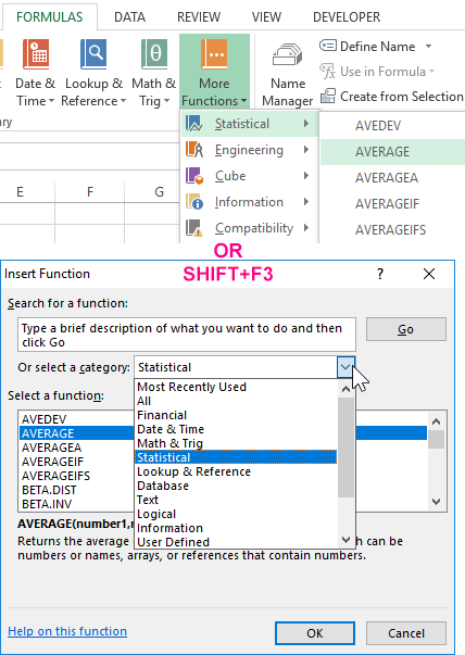
- The second method is based on the same principle of finding the arithmetic mean. But we will call the function AVERAGE differently. Using the function wizard (use fx button or key combination SHIFT + F3).
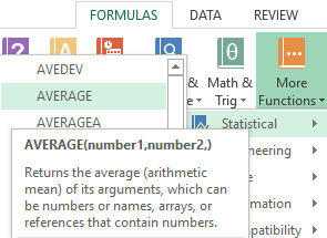
- The third way to call the AVERAGE function from the panel: «FORMULAS»-«More Function»-«Statistical»-«AVERAGE».
Or you can make cell to be active and just manually enter the formula: =AVERAGE(A1:A8).
Now let’s see what the AVERAGE function be able to:
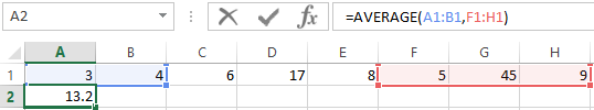
Let us find the arithmetic mean of the first two and three last numbers. Formula: =AVERAGE(A1:B1,F1:H1).
Average value by condition
A numerical criterion or a textual criterion can be the condition for finding the arithmetic mean. We will use the function: = AVERAGEIF().
Find the arithmetic mean for numbers that are greater or equal to 10.
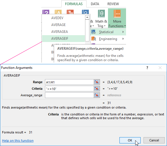
The result of using the function «AVERAGEIF» by the condition «>=10» is next:
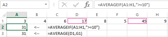
The third argument «Averaging Range» is omitted. Firstly, it is not necessary. Secondly, the range analyzed by the program contains ONLY numeric values. In the cells specified in the first argument, the search will be performed according to the condition specified in the second argument.
Attention! You can specify the search criteria in the cell. And in the formula make a reference to it.
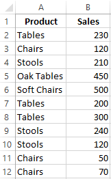
Let’s find the average value of numbers by the text criterion. For example, the average sales of goods «Tables».
The function will look like this:
Range is a column with the names of goods. Search criteria is a link to a cell with the word «Tables» (you can insert the word «Tables» instead of the A7 link). The averaging range is the cells from which data will be taken to calculate the arithmetic mean.
We get the following value as a result of calculating using the function:
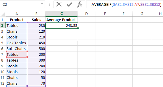
Attention! It is mandatory to point the averaging range for the text criterion (condition).
How to calculate the weighted average price in Excel?
How to calculate the average percentage in Excel? For this purpose, the SUMPRODUCTS and SUM functions are suitable. Table for an example:
How did we know the weighted average price?
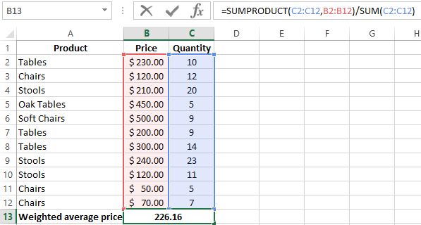
Using the formula =SUMPRODUCT() we learn the total revenue after the realization of the entire quantity of goods. And the =SUM() function sums the goods quantity. We found a weighted average price having divided the total revenue from the sale of goods by the total number of units of the goods. This indicator takes into account the «weight» of each price and its share in the total mass of values.
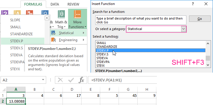
The standard deviation: the formula in Excel
There is a standard deviation in the entire population and in the sampling. In the first case, this is the square root of the general variance. In the second, this is a square root of the sampling variance.
A dispersion formula is compiled to calculate this statistical indicator. The square root is extracted from it. But in Excel, there is a ready-made function for finding the root-mean-square deviation.
The root-mean-square deviation is related to the scope of the initial data. This is not enough for a figurative representation of the variation of the analyzed range. The coefficient of variation is calculated to obtain the relative level of the data variability.
standard deviation / arithmetic mean
The formula in Excel is as follows:
STDEV.P (range of values) / AVERAGE (range of values).
The coefficient of variation is considered as a percentage. Therefore, set the percentage format in the cell set.
Источник
AVERAGE Function
Summary
The Excel AVERAGE function calculates the average (arithmetic mean) of supplied numbers. AVERAGE can handle up to 255 individual arguments, which can include numbers, cell references, ranges, arrays, and constants.
Purpose
Return value
Arguments
- number1 — A number or cell reference that refers to numeric values.
- number2 — [optional] A number or cell reference that refers to numeric values.
Syntax
Usage notes
The AVERAGE function calculates the average of numbers provided as arguments. To calculate the average, Excel sums all numeric values and divides by the count of numeric values.
AVERAGE takes multiple arguments in the form number1, number2, number3, etc. up to 255 total. Arguments can include numbers, cell references, ranges, arrays, and constants. Empty cells, and cells that contain text or logical values are ignored. However, zero (0) values are included. You can ignore zero (0) values with the AVERAGEIFS function, as explained below.
The AVERAGE function will ignore logical values and numbers entered as text. If you need to include these values in the average, see the AVERAGEA function.
If the values given to AVERAGE contain errors, AVERAGE returns an error. You can use the AGGREGATE function to ignore errors.
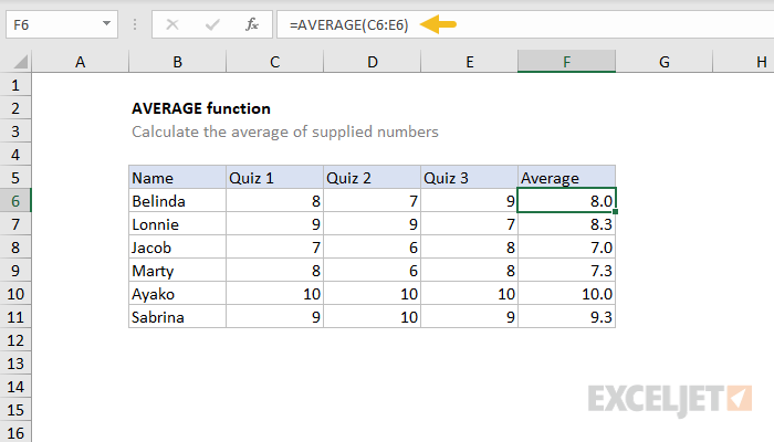
Basic usage
A typical way to use the AVERAGE function is to provide a range, as seen below. The formula in F3, copied down, is:

At each new row, AVERAGE calculates an average of the quiz scores for each person.
Blank cells
The AVERAGE function automatically ignores blank cells. In the screen below, notice cell C4 is empty, and AVERAGE simply ignores it and computes an average with B4 and D4 only:
![]()
However, note the zero (0) value in C5 is included in the average, since it is a valid numeric value. To exclude zero values, use AVERAGEIF or AVERAGEIFS instead. In the example below, AVERAGEIF is used to exclude zero values. Like the AVERAGE function, AVERAGEIF automatically excludes empty cells.

Mixed arguments
The numbers provided to AVERAGE can be a mix of references and constants:

Average with criteria
To calculate an average with criteria, use AVERAGEIF or AVERAGEIFS. In the example below, AVERAGEIFS is used to calculate the average score for Red and Blue groups:

The AVERAGEIFS function can also apply multiple criteria.
Average top 3
By combining the AVERAGE function with the LARGE function, you can calculate an average of top n values. In the example below, the formula in column I computes an average of the top 3 quiz scores in each row:

Weighted average
To calculate a weighted average, you’ll want to use the SUMPRODUCT function, as shown below:
Average without #DIV/0!
The average function automatically ignores empty cells in a set of data. However, if the range contains no numeric values, AVERAGE will return a #DIV/0! error. To avoid this problem, you can check the count of values with the COUNT function and the IF function like this:
When the count of numeric values is zero, IF returns an empty string («»). When the count is greater than zero, AVERAGE returns the average. This example explains this idea in more detail.
Manual average
To calculate the average, AVERAGE sums all numeric values and divides by the count of numeric values. This behavior can be replicated with the SUM and COUNT functions manually like this:
Источник
На чтение 1 мин
Функция СРЗНАЧ в Excel используется для вычисления среднего арифметического из заданного диапазона данных.
Содержание
- Что возвращает функция
- Синтаксис
- Аргументы функции
- Дополнительная информация
- Примеры использования функции СРЗНАЧ в Excel
Что возвращает функция
Возвращает число, соответствующее среднему арифметическому от заданного диапазона данных.
 Больше лайфхаков в нашем Telegram Подписаться
Синтаксис
=AVERAGE(number1, [number2], …) — английская версия
=СРЗНАЧ(число1;[число2];…) — русская версия
Аргументы функции
- number1 (число1) — первое число, диапазон чисел, из которого необходимо вычислить среднее арифметическое;
- [number2] ([число2]) (Опционально) — второе число, диапазон чисел, из которого необходимо вычислить среднее арифметическое. Максимальное количество аргументов функции — 255.
Дополнительная информация
- Аргументами функции СРЗНАЧ (AVERAGE) в Excel могут быть числа, именованные диапазоны, ссылки на ячейки, содержащие числовые значения;
- Ссылки на ячейки содержащими текст, логические значения или пустые ячейки игнорируются функцией. Вместе с тем, ячейки со значением «0» учитываются при вычислении среднего арифметического;
- Учитываются логические значения и текстовые представления чисел, которые вы вводите непосредственно в список аргументов;
- Аргументы с ошибками не могут быть учтены и использованы при работе функции.
Примеры использования функции СРЗНАЧ в Excel
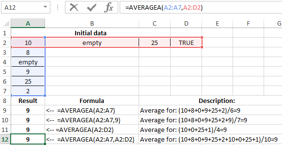
AVERAGE and AVERAGEA functions are used to calculate the arithmetic average of the arguments of interest in Excel. The average is calculated in the classical way — summing all the numbers and dividing the sum by the number of these numbers. The main difference between these functions is that they process differently non-numeric types of values that are in Excel cells. More about everything in more detail.
Examples of using the AVERAGE function in Excel
AVERAGE function refers to the Statistical group. Therefore, to call this function in Excel, you must select the tool: “FORMULAS” — “Functions Library” — “More functions” — “Statistical” — “AVERAGE”. Or call the «Insert Function» dialog box (SHIFT + F3) and select the «Statistical» option from the «Category:» drop-down list. After that, in the “Select function:” field there will be a list of categories with statistical functions where the AVERAGE is located, as well as AVERAGEA.
If there is a range of B2:B8 cells with numbers, then the formula =AVERAGE(B2:B8) will return the average value of the given numbers in this range:
The syntax is the following: =AVERAGE(number1,[number2],…), where the first number is a required argument, and all subsequent arguments (up to the number 255) are optional for filled. That is, the number of selected source ranges cannot exceed more than 255:
The argument can have a numeric value, be a reference to a range or array. Text and logical values in the range are completely ignored.
The arguments of the AVERAGE function can be represented not only by numbers, but also by names or references to a specific range (cell) containing a number. The logical value and textual representation of the number, which is directly entered into the argument list, is taken into account.
If the argument is represented by a reference to a range (cell), then its text or logical value (reference to an empty cell) is ignored. In this case, cells that contain zero are counted. If the argument contains errors or text that cannot be converted to a number, then this results in a common error. To take into account logical values and the textual representation of numbers, it is necessary to use in the calculations the AVERAGEA function, which will be discussed further.
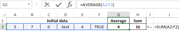
The result of the function in the example in the picture below is the number 4, since logical and text objects are ignored. Therefore:
(5 + 7 + 0 + 4) / 4 = 4
When calculating averages, you need to take into account the difference between a blank cell and a cell containing a zero value, especially if the «Show a zero in cells that have zero values» option is cleared in the Excel dialog box. When checked, empty cells are ignored, but zero values are not. To remove or set this flag, open the “FILE” tab, then click on “Options” and select in the category “Advanced” group “Display options for this worksheet:”, where it is possible to check the box:
The results of another 4 tasks are summarized in the table below:
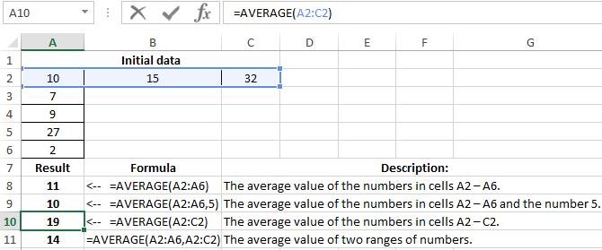
As you can see in the example, in cell A9, the AVERAGE function has 2 arguments: 1 — a range of cells, 2 — an additional number 5. The same can be specified in the arguments and additional ranges of cells with numbers. For example, as in cell A11.
Formulas with examples of using the AVERAGEA function
AVERAGEA function differs from AVERAGE in that the true logical value of “TRUE” in the range is equal to 1, and the false logical value of “FALSE” or the text value in the cells is equal to zero. Therefore, the result of calculating the AVERAGEA function is different:
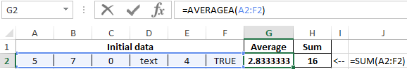
The result of the function returns the number in the example 2,833333, since the text and logical values are taken as zero, and the logical TRUE is equal to one. Consequently:
(5 + 7 + 0 + 0 + 4 + 1) / 6 = 2.83
Syntax:
=AVERAGEA(value1,[value2],…)
The arguments of the AVERAGEA function are subject to the following properties:
- «Value1» is mandatory, and «value2» and all values that follow it are optional. The total number of cell ranges or their values can be from 1 to 255 cells.
- The argument can be a number, a name, an array, or a reference containing a number, as well as a textual representation of the number or a logical value, for example, “true” or “false”.
- The logical value and textual representation of the number entered in the argument list is taken into account.
- An argument containing the value “true” is interpreted as 1. An argument containing the value “false” is interpreted as 0 (zero).
- Text contained in arrays and references is interpreted as 0 (zero). An empty text («») is also interpreted as 0 (zero).
- If the argument is an array or reference, then only the values included in this array or reference are used. Empty cells and text in the array and reference are ignored.
- Arguments that are error values or text that cannot be converted to numbers cause errors.
The results of the feature of AVERAGEA are summarized in the table below:
Download examples with functions AVERAGE for Excel
Attention! When calculating the mean values in Excel, you need to take into account the differences between a blank cell and a cell containing a zero value (especially if the “Show a zero in cells that have zero values” in “Option” is unchecked in the options dialog box). When checked, empty cells are not counted, and zero values are counted. To check the box on the “FILE” tab, select the “Option” command, go to the “Advanced” category, where find the section “Show options for the next sheet” and set the flag there.