Do not sum duplicates in excel

Data analysis usually involves large data sets, and at some point, one may need to find out the number of values that appear only once in the dataset. In this case, you will be counting without duplicates. Unique values are values that appear only once in a dataset.

If you are faced with mountains of data, then counting without duplicates might be very arduous. More so, Excel does not have a special formula for counting without duplicates. However, there is always a way out! This tutorial will serve as a guide on how to count unique and distinct values without duplicating them.

Take a look at the numbers in the table above; the unique values are not duplicated. They don’t appear more than once. Whereas, distinct values are the different numbers in the collection. In the table below, we have separated the unique values from distinct values.

1. Using the array COUNTIF formula

The COUNTIF function counts the frequency of occurrence of each value within the range. To get the number of the unique values, you have to sum them up. You can do this efficiently by combining SUM and COUNTIF functions. A combo of two functions can count unique values without duplication.

Below is the syntax:

=SUM(IF(COUNTIF(data, data)=1,1,0)).

The formula contains three separate functions – SUM, IF, and COUNTIF.

COUNTIF function» counts how many times a particular number appears within the range.

«IF function» analysis the results returned by the «COUNTIF» function. It maintains the 1’s for unique values and replaces other values with «0.»

Note: Always press Ctrl + Shift + Enter when entering your array formula.

CTRL+SHIFT+ENTER allow excel to recognize the formula as an array function.  unique value= =SUM(IF(COUNTIF(A2:A10, A2:A10)=1,1,0))

Alternatively, you can use the SUMPRODUCT formula to avoid the use of CTRL+SHIFT+ENTER.

Below is the syntax:

=SUMPRODUCT(1/COUNTIF(range, criteria)).

In the example below, we have a list of items with duplicates.

If we use the SUM formula to count the total number of items, there will be duplicates. To exclude the duplicates, you have to follow these steps.

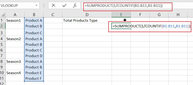
Step 1: Go to cell D1 and enter this formula “=SUMPRODUCT(1/COUNTIF( B1:B11,B1:B11)). B1:B11 is the array range you want to count the total number of unique values in the list.

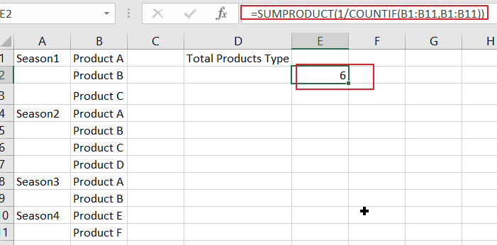
Step 2: Press enter and the results will be displayed in cell D1. From the displayed results (6) we can see there are no duplicates.

The above formula counts the values of the six items A/B/C/D/E/F.  

2. Using a combination of SUM, IF, FREQUENCY, MATCH, and ROW Function

If we want to count unique values that exclude all duplicates (that appear in more than one product), use the combination of these functions.

• The sum function allows you to add the values.
• For each true condition of IF function, assign value 1.
• The FREQUENCY function allows you to count the number of values ignoring texts and zeros. In the first occurrence of the distinct value, it returns an equal number to the number of occurrences of that value. It returns zero for the occurrences that have the same value after the first occurrence.
• The MATCH function returns the position of the text value in an array range. The return value acts as the function argument for FREQUENCY.
• The ROW function returns the row reference number. 

Example: Enter the following formula to count unique values by excluding all duplicates

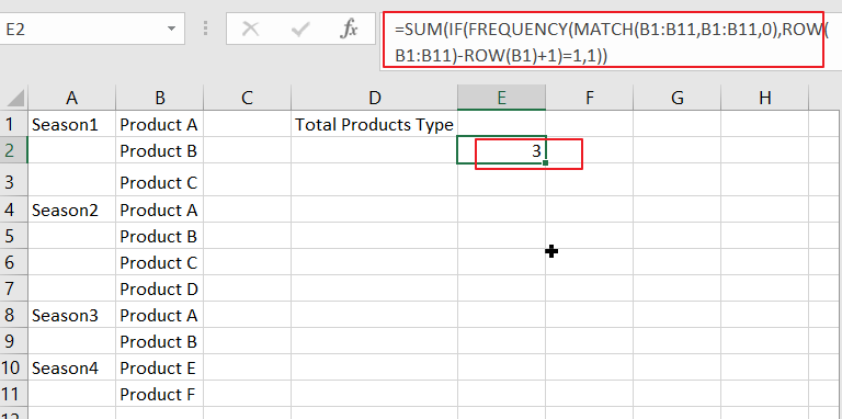
=SUM(IF(FREQUENCY(MATCH(B1:B11,B1:B11,0),ROW(B1:B11)-ROW(B1)+1)=1,1))

Press enter. The unique value is 3 (Item D/E/F).

3. Using ISNUMBER Function to count numeric numbers

The function we used earlier counts, both texts and numbers, without duplicating. To count only numerals without duplicating, you have to include ISNUMBER function in the formula for finding unique values.

=SUM(IF(ISNUMBER(A2:A10)*COUNTIF(A2:A10,A2:A10)=1,1,0))

Note: Always press Ctrl + Shift + Enter when entering your array formula.

Meanwhile, the lowdown in this function is that it also counts dates and times.

4. Using ISTEXT Function to count text values

You can count the number of texts without duplicating by including the ISTEXT function in the array formula as stated below:

=SUM(IF(ISTEXT(A2:A10)*COUNTIF(A2:A10,A2:A10)=1,1,0))

This formula will display the number of unique texts. It excludes errors, blank cells, logical numbers, numbers, etc.

Always press Ctrl + Shift + Enter when entering your array formula.

5. Using Pivot Table to count text values

Easies way to count the value is by creating the pivot table and using the Count of items

1. Create a pivot table

2. Use Count of Items

3. Output Table

6. Using A Filter

The Filter method is the simplest approach that allows you to remove duplicates and remain with unique values. You can, therefore, use two tricks to get unique values as discussed below.

6.1: Filtering for Unique Values

Steps:

1. Select and make sure the range of cells you want to make unique is in a table.

2. Click on Data then select the Advanced option in the soft & filter group.

3. When the Advanced Filter box pops up, you can filter the range of cells or tables by clicking on the Filer the List, in-place option.

4. You can also copy the result of the filter to another location by clicking on the Copy to another location option.

5. Enter a cell reference in the Copy To box.

6. Alternatively, you can click the Collapse Dialog option to hide the popup window temporarily, select a cell on the worksheet, and then click the Expand option.

7. Finish by checking the Unique Records Only and click OK.

6.2: Removing The Duplicates

The method only affects the values in the range of cells or tables and not values outside. After removing the duplicates, you will keep the first occurrence of the value in the list, while the identical values will be deleted. Therefore, remember to copy the original range of cells to the table to another worksheet before deleting duplicates.

Steps:

1. Start by selecting the active range of cells in a table.

2. Select the Data Tab and click Remove Duplicates in the Data Tools group.

3. You can select one or more columns under the Columns face. Alternatively, you can click Select All to select all columns quickly or Unselect All to clear all columns quickly.

4. Click OK and a message will pop up showing how many duplicates you have removed or how many unique values remain. To dismiss the message, click OK.

5. You can undo the change by clicking Undo or pressing Ctrl + Z

7. Using Amazing Excel Tools

Another simple way to count without duplicates in excel is tools like Kutools by the following steps.

1. Select a blank cell to output the result.

2. Click Kutools>Formula>Helper>Formula Helper.

3. Do the following steps in the formula helper dialog;

• Check and select Count unique values in the Choose a formula box. You can check the filter box and type some words to filter the formula names.
• Then choose the range in which you want to count unique values in the range box.
• Press the OK button.

8. Using A Data Model with A Pivot Table to Count Unique Values

The method applies to newer versions of Microsoft Excel, including Microsoft 365, Excel 2019, Excel 2016, and Excel 2013. To count unique values using this approach, follow these steps:

1. Select any cell in the data and click on the Insert tab in the ribbon.

2. Click on Pivot Table to open a dialogue box.

3. Select the Add this data to the Data Model at the bottom and click OK.

4. In the resulting window, drag the Name column into the Name field and the Profession column or any other in the dataset into the Values field.  

5. Click on the small arrow next to the Count of Profession option in the Pivot Table fields.

6. Select the Value Field Settings at the bottom.

7. Finish by selecting the Distinct Count or Unique Count option and click OK.

8. You will have your unique values in the Pivot Table.

9. Using Power Pivot

Power Pivot is also another powerful method you can use to count unique values. However, you will need an enabled Power Pivot tab in your ribbon. That means if your Excel version does not have an already-enabled Power Pivot add-in, you will have to enable it first. Once you have enabled it, you can proceed with the following steps:

1. Go to the Data Model and select the Manage Button.

2. This will open a new blank window if it is your first time importing data.

3. Click on Home Tab and select the “Get External Data” option.

4. You will see various sources and options to upload data. Since you want to upload simple Excel, select the «From Other Sources» option.

5. Scroll down to the end of a new dialogue box opened, select “Excel File”, and click Next.

6. You will need to rename the connection created. For simplicity, you can rename it “Excel”. After that, click on “Browse” to choose an Excel file path.

7. You can click on the “Use the first row as column header” option to make the top column the header. Click on the Next Button to finish.

8. You will see the file imported to the Data Model. Click the Finish button.

9. After importing all the rows successfully, hit the Close Button.

10. With your new worksheet, you will have to create a Pivot Table by clicking on Home and then Pivot Table.

11. Click on the small triangle next to it to expand the columns. That is because you already have the data on the first sheet.

12. After dragging and dropping all the data in their respective fields, you will get a simple Pivot Table.

13. Go back to the Power Pivot window and select the Measure option to create a New Measure.

14. Add your desired description name by typing in the box and the suggestions will pop up automatically. Since you want to count unique values, select the Unique Count function.

15. Press the Tab button or use the bracket to select which column you need the unique count for. For example, if you want the unique count for Profession, your formula will be like this;

=DISTINCTCOUNT (Sheet1[Profession]))

16. Select the Number category since you want to count unique values.

17. Change the format to “Whole Number’ and hit OK to create a new column with unique entries.

I hope this tutorial is comprehensive. Kindly share with friends & thanks for reading!

Combine duplicate rows and sum the values with Consolidate function

1. Click a cell where you want to locate the result in your current worksheet.
2. Go to click Data > Consolidate, see screenshot:
3. In the Consolidate dialog box:
4. After finishing the settings, click OK, and the duplicates are combined and summed.

Can I combine duplicates in Excel?

In Excel, there is often a need to combine duplicate rows in a range and sum them in a separate column.In the Consolidate window, leave the default Function (Sum), and click on the Reference icon to select a range for consolidation. 3. Select the data range you want to consolidate (e.g., B1:C17), and click Enter.

How do I sum duplicate values in Excel using Vlookup?

Vlookup and sum matches in a row or multiple rows with formulas

1. =SUM(VLOOKUP(A10, $A$2:$F$7, {2,3,4,5,6}, FALSE))
2. Notes:
3. =SUMPRODUCT((A2:A7=A10)*B2:F7)
4. =SUM(INDEX(B2:F7,0,MATCH(A10,B1:F1,0)))

How do you sum in Excel without duplicates?

Count Unique Values Excluding All Duplicates by Formula in Excel. Step 1: In E2 which is saved the total product type number, enter the formula “=SUM(IF(FREQUENCY(MATCH(B1:B11,B1:B11,0),ROW(B1:B11)-ROW(B1)+1)=1,1))”, B1:B11 is the range you want to count the unique values. Step2: Click Enter and get the result in E2.

How do I sum values from a group in Excel?

Sum values by group with using formula
Select next cell to the data range, type this =IF(A2=A1,””,SUMIF(A:A,A2,B:B)), (A2 is the relative cell you want to sum based on, A1 is the column header, A:A is the column you want to sum based on, the B:B is the column you want to sum the values.)

How do you use Sumif formula?

If you want, you can apply the criteria to one range and sum the corresponding values in a different range. For example, the formula =SUMIF(B2:B5, “John”, C2:C5) sums only the values in the range C2:C5, where the corresponding cells in the range B2:B5 equal “John.”

What is an Xlookup in Excel?

Use the XLOOKUP function to find things in a table or range by row.With XLOOKUP, you can look in one column for a search term, and return a result from the same row in another column, regardless of which side the return column is on.

How do you highlight duplicates in Excel?

Find and remove duplicates

1. Select the cells you want to check for duplicates.
2. Click Home > Conditional Formatting > Highlight Cells Rules > Duplicate Values.
3. In the box next to values with, pick the formatting you want to apply to the duplicate values, and then click OK.

How do I count only duplicate names in Excel?

Part 2: Count Duplicate Values Once with Case Insensitive
This time we count number with case insensitive. Step 1: In B2 enter the formula =SUMPRODUCT((A2:A11<>””)/COUNTIF(A2:A11,A2:A11&””)). Step 2: Press Enter directly to get result.

How do I merge duplicates in Excel without losing data?

Combine rows in Excel with Merge Cells add-in

1. Select the range of cells where you want to merge rows.
2. Go to the Ablebits Data tab > Merge group, click the Merge Cells arrow, and then click Merge Rows into One.
3. This will open the Merge Cells dialog box with the preselected settings that work fine in most cases.

How do I combine unique data in Excel?

How to merge duplicate rows in Excel

1. On Step 1 select your range.
2. On Step 2 choose the key columns with duplicate records.
3. On Step 3 indicate the columns with the values to merge and choose demiliters.
4. All the duplicates are merged according to the key columns.

How do I merge and delete duplicates in Excel?

Remove Duplicates

1. Open a workbook with two worksheets you’d like to merge.
2. Select all data in the first worksheet, and then press “Ctrl-C” to copy it to the clipboard.
3. Select all data in the new workbook, and then click the Data tab’s “Remove Duplicates” command, located in the Data Tools command group.

How do I SUM rows and groups in Excel?

To group rows or columns:

1. Select the rows or columns you want to group. In this example, we’ll select columns A, B, and C.
2. Select the Data tab on the Ribbon, then click the Group command. Clicking the Group command.
3. The selected rows or columns will be grouped. In our example, columns A, B, and C are grouped together.

What is sum range in Excel?

The Excel SUMIF function returns the sum of cells that meet a single condition. Criteria can be applied to dates, numbers, and text.sum_range – [optional] Range to sum. If omitted, cells in range are summed.

How do you sum text in Excel?

In the Choose a formula list box, click to select Sum based on the same text option; Then, in the Arguments input section, select the range of cells containing the text and numbers that you want to sum in the Range textbox, and then, select the text cell you want to sum values based on in the Text textbox.

Is Xlookup better than VLOOKUP?

The XLOOKUP defaults to an exact match where the VLOOKUP defaults to an approximate match. As the exact match is used most often, this setting would make the XLOOKUP more effective. On top of this, the XLOOKUP offers an additional option of an approximate match returning the next larger value.

Is Xlookup better than index match?

Performance of XLOOKUP vs. INDEX/MATCH and INDEX/XMATCH.Because calculation times for VLOOKUP and INDEX/MATCH are on a similar level, the performance of XLOOKUP compared to INDEX/MATCH doesn’t surprise much: XLOOKUP is significantly slower than INDEX/MATCH as well. But more: Excel also has a new XMATCH function.

How do I use xmatch in Excel?

The Excel XMATCH function performs a lookup and returns a position.
Excel XMATCH Function

1. lookup_value – The lookup value.
2. lookup_array – The array or range to search.
3. match_mode – [optional] 0 = exact match (default), -1 = exact match or next smallest, 1 = exact match or next larger, 2 = wildcard match.

How do I highlight duplicate colors in Excel?

Select the data range you want to color the duplicate values, then click Home > Conditional Formatting > Highlight Cells Rules > Duplicate Values.

1. Then in the popping dialog, you can select the color you need to highlight duplicates from the drop down list of values with.
2. Click OK.

How do I highlight duplicates in sheets?

Google Sheets: How to highlight duplicates in a single column

1. Open your spreadsheet in Google Sheets and select a column.
2. For instance, select column A > Format > Conditional formatting.
3. Under Format rules, open the drop-down list and select Custom formula is.
4. Enter the Value for the custom formula, =countif(A1:A,A1)>1.

How do I count unique values in Excel?

Count the number of unique values by using a filter

1. Select the range of cells, or make sure the active cell is in a table.
2. On the Data tab, in the Sort & Filter group, click Advanced.
3. Click Copy to another location.
4. In the Copy to box, enter a cell reference.
5. Select the Unique records only check box, and click OK.

Are you able to add another column for additional criteria?

For example, if you add another column (let’s say it’s in column A) with the formula

=IF(COUNTIF($R$50:R50,R50)=1,1,0)

The formula above will return a 1 if the value in Cell R50 is unique, and a 0 if it is not. Now change your SumIf function to SumIfs. You could use

=SUMIFS($AG$50:$AG$54,$R$50:$R$54,R50,$A$50:$A$54,1)

to return the sum of only unique values.

The SumIfs function is pretty much a SumIf function, but with the ability to use multiple criteria without the need for an array function. SumIf criteria is SUMIFS(sum_range, criteria_range1, criteria1, [criteria_range2, criteria2], ...), so we are returning the sum of all values in AG50:AG54 where the value in R50:R54 matches that of R50 AND the unique flag in A50:A54 equals 1.

Edit
I should clarify that the SUMIFS formula isn’t available in Office 2003 and below. If this means you cannot use SUMIFS, I believe you will need an array formula, let me know.

We enter a list of numbers or products and there are some duplicates in the list, if we want to just do count for the unique values and exclude the duplicates, how can we do? Now you can follow the below steps to solve this question by formula quickly.

Prepare a list of products and there are some duplicates among the list. See example below:

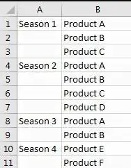
And we want to count the total product type in one year, how can we do count?

If we just use sum formula to do count, then duplicates will be included, so we need another formula to do count excludes the duplicates. See steps below.

Step 1: In E2 which is saved the total product type number, enter the formula:

=SUMPRODUCT(1/COUNTIF(B1:B11,B1:B11))

Where B1:B11 is the range you want to count the unique values.

Step 2: Click Enter and get the result in E2. We can check the result is 6, and the duplicates are not included.

In above sample, we do count for unique values and get the result 6, because we have six products ABCDEF, and if we want to only count the unique values exclude all duplicates like product ABC (they appeared more than one season) how can we do count? See below steps.

2. Count Unique Values Excluding All Duplicates by Formula in Excel

Step 1: In E2 which is saved the total product type number, enter the formula:

=SUM(IF(FREQUENCY(MATCH(B1:B11,B1:B11,0),ROW(B1:B11)-ROW(B1)+1)=1,1))

Where B1:B11 is the range you want to count the unique values.

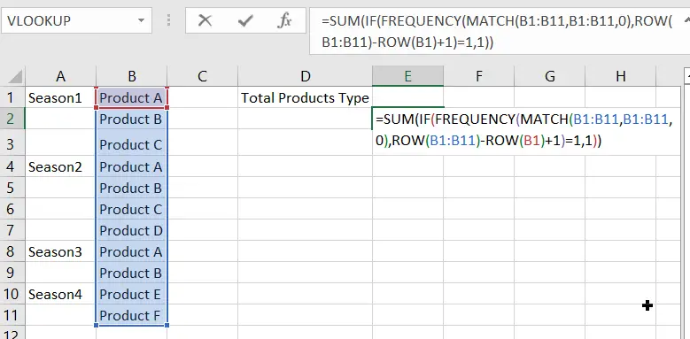
Step2: Click Enter and get the result in E2. We can check the result is 3 (Product DEF are unique values and only appeared in one season).

3. Video: Count Only Unique Values Excluding Duplicates

If you want to learn how to count only unique values excluding duplicates in Excel, this video will show you a simple and effective formula that you can use in any situation.

• Excel SUMPRODUCT function
  The Excel SUMPRODUCT function multiplies corresponding components in the given one or more arrays or ranges, and returns the sum of those products.The syntax of the SUMPRODUCT function is as below:= SUMPRODUCT (array1,[array2],…)…
• Excel COUNTIF function
  The Excel COUNTIF function will count the number of cells in a range that meet a given criteria. This function can be used to count the different kinds of cells with number, date, text values, blank, non-blanks, or containing specific characters.etc.= COUNTIF (range, criteria)…
• Excel ROW function
  The Excel ROW function returns the row number of a cell reference.The ROW function is a build-in function in Microsoft Excel and it is categorized as a Lookup and Reference Function.The syntax of the ROW function is as below:= ROW ([reference])….
• Excel MATCH function
  The Excel MATCH function search a value in an array and returns the position of that item.The syntax of the MATCH function is as below:= MATCH  (lookup_value, lookup_array, [match_type])…
• Excel IF function
  The Excel IF function perform a logical test to return one value if the condition is TRUE and return another value if the condition is FALSE. The IF function is a build-in function in Microsoft Excel and it is categorized as a Logical Function.The syntax of the IF function is as below:= IF (condition, [true_value], [false_value])….
• Excel SUM function
  The Excel SUM function will adds all numbers in a range of cells and returns the sum of these values. You can add individual values, cell references or ranges in excel.The syntax of the SUM function is as below:= SUM(number1,[number2],…)…