
This formula will count only numbers <> 0, excluding blanks, error messages, etc. BUT it will not exclude the cells that display ###### (but really contain a number) if the reason for that is a column that is too narrow, or a negative date or time value.
=SUMPRODUCT(--ISNUMBER(A2:A200))-COUNTIF(A2:A200,0)
If you really want to avoid counting cells that display ####### when the underlying contents is a number not equal to zero, you will need to use a UDF to act on the Text property of the cell. In addition, narrowing or widening the column to produce that affect will not trigger a calculation event that would update the formula, so you need to somehow do that in order to ensure the formula results are correct.
That is why I added Application.Volatile to the code, but it is still possible to produce a situation where the result of the formula does not agree with the display in the range being checked, at least until the next calculation event takes place.
To enter this User Defined Function (UDF), alt-F11 opens the Visual Basic Editor.
Ensure your project is highlighted in the Project Explorer window.
Then, from the top menu, select Insert/Module and
paste the code below into the window that opens.
To use this User Defined Function (UDF), enter a formula like
=CountNumbersNEZero(A2:A200)
in some cell.
Option Explicit
Function CountNumbersNEZero(rg As Range) As Long
Application.Volatile
    Dim C As Range
    Dim L As Double
For Each C In rg
    If IsNumeric(C.Text) Then
        If C.Text <> 0 Then L = L + 1
    End If
Next C
CountNumbersNEZero = L
End Function
Предположим, у вас есть диапазон данных, который включает несколько нулевых значений и пустых ячеек, как показано на скриншоте ниже, и ваша задача — подсчитывать ячейки, игнорируя как нулевые значения, так и пустые ячейки, как вы можете быстро их правильно подсчитать?

 Подсчет без учета нулей и пустых ячеек с формулой
Вот формула со стрелкой, которая поможет вам подсчитать ячейки, игнорируя нули и пустые ячейки.
Выберите пустую ячейку, в которую вы хотите поместить результат подсчета, и введите эту формулу =COUNT(IF(A1:E5<>0, A1:E5)) в это нажмите Shift + Ctrl + Enter ключ для получения результата.

![]()
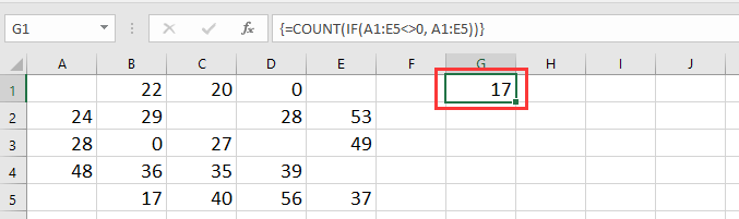
Совет: В формуле A1: E5 — это диапазон ячеек, который вы хотите подсчитать, игнорируя пустые ячейки и нулевые значения.
Считайте, игнорируя нули и пустые ячейки с помощью Kutools for Excel
Если вы хотите подсчитать ячейки, исключая нули и пустые ячейки, а затем выбрать их, вы можете применить Kutools for ExcelАвтора Выбрать определенные ячейки чтобы быстро с этим справиться.
После бесплатная установка Kutools for Excel, пожалуйста, сделайте следующее:
1. Выберите ячейки, которые нужно подсчитать, и нажмите Кутулс > Выберите > Выбрать определенные ячейки. Смотрите скриншот:
2. в Выбрать определенные ячейки диалог, проверьте Ячейка под Тип выбора раздел и выберите Не равно критерий из первого раскрывающегося списка под Конкретный тип раздел, затем введите 0 в следующее текстовое поле. Смотрите скриншот: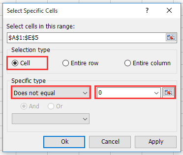
3. Нажмите Ok or Применить, теперь появляется диалоговое окно, напоминающее вам, сколько ячеек выбрано, и тем временем были выбраны все ячейки, за исключением нулевых значений и пустых ячеек.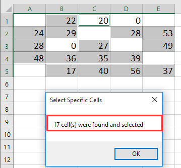
Щелкните здесь, чтобы узнать больше о выборе конкретных ячеек.
Подсчет без учета пустых ячеек только со строкой состояния
Если вы хотите, чтобы подсчет ячеек игнорировал только пустые ячейки, вы можете выбрать ячейки, а затем просмотреть результат подсчета в строке состояния.
Выберите ячейки, в которых вы хотите подсчитать только ячейки, за исключением пустых ячеек, а затем перейдите в правый нижний угол строки состояния, чтобы просмотреть результат подсчета. Смотрите скриншот: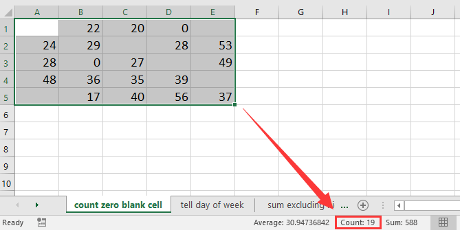
- Как посчитать в Excel ячейки с нулями, но не с пробелами?
- Как посчитать / суммировать ячейки по цветам с условным форматированием в Excel?
- Как посчитать количество символов, букв и цифр в ячейке?
- Как посчитать количество листов в рабочей тетради?
Лучшие инструменты для работы в офисе
Kutools for Excel Решит большинство ваших проблем и повысит вашу производительность на 80%
- Снова использовать: Быстро вставить сложные формулы, диаграммы и все, что вы использовали раньше; Зашифровать ячейки с паролем; Создать список рассылки и отправлять электронные письма …
- Бар Супер Формулы (легко редактировать несколько строк текста и формул); Макет для чтения (легко читать и редактировать большое количество ячеек); Вставить в отфильтрованный диапазон…
- Объединить ячейки / строки / столбцы без потери данных; Разделить содержимое ячеек; Объединить повторяющиеся строки / столбцы… Предотвращение дублирования ячеек; Сравнить диапазоны…
- Выберите Дубликат или Уникальный Ряды; Выбрать пустые строки (все ячейки пустые); Супер находка и нечеткая находка во многих рабочих тетрадях; Случайный выбор …
- Точная копия Несколько ячеек без изменения ссылки на формулу; Автоматическое создание ссылок на несколько листов; Вставить пули, Флажки и многое другое …
- Извлечь текст, Добавить текст, Удалить по позиции, Удалить пробел; Создание и печать промежуточных итогов по страницам; Преобразование содержимого ячеек в комментарии…
- Суперфильтр (сохранять и применять схемы фильтров к другим листам); Расширенная сортировка по месяцам / неделям / дням, периодичности и др .; Специальный фильтр жирным, курсивом …
- Комбинируйте книги и рабочие листы; Объединить таблицы на основе ключевых столбцов; Разделить данные на несколько листов; Пакетное преобразование xls, xlsx и PDF…
- Более 300 мощных функций. Поддерживает Office/Excel 2007-2021 и 365. Поддерживает все языки. Простое развертывание на вашем предприятии или в организации. Полнофункциональная 30-дневная бесплатная пробная версия. 60-дневная гарантия возврата денег.
")
Вкладка Office: интерфейс с вкладками в Office и упрощение работы
- Включение редактирования и чтения с вкладками в Word, Excel, PowerPoint, Издатель, доступ, Visio и проект.
- Открывайте и создавайте несколько документов на новых вкладках одного окна, а не в новых окнах.
- Повышает вашу продуктивность на 50% и сокращает количество щелчков мышью на сотни каждый день!
")
Комментарии (0)
Оценок пока нет. Оцените первым!
Excel has special functions to calculate the average of the number in a range of cells and also calculate the average of cells based on specified criteria, like AVERAGE and AVERAGEIF functions. But there are situations where cells in a range are Blank or may contain zeros, so it may affect the result. So you need to take Excel average without zeros and average if not blank. In this case, you need to use AVERAGEIF function to average cells based on criteria.
The AVERAGEIF function in Excel
AVERAGEIF function averages cells based on supplied criteria in Excel as per its syntax. The syntax of AVERAGEIF function is as follows;
=AVERAGEIF (range, criteria, [average_range])
Here,
range – This argument contains the range of cells on which criteria are tested.
criteria – This argument contains the condition to determine which cells to average. It may contain numeric or text values, a logical expression, cell reference or other functions as the condition to meet.
average_range – This argument consists of the range of cells that contain numbers you want to average. It is the optional argument and if you omit this argument in function then function averages cells given in range argument.
Ignore zeros when finding the average
In this case, as you need to average ignoring zeros in a range argument, so you do not need to supply average_range argument in the AVERAGEIF function here. You need to supply only range argument and criteria argument to find the average.
In the criteria argument, you need to test the criteria “Not Equal to Zero”. This is done by using logical expression Not Equal To (<>) with Zero, enclosed in double quotation marks (“”).
Ignore Blanks When Finding the Average
Remember that like AVERAGE function, AVERAGEIF function automatically ignores Blank cells and cells containing text values. So you do not need to make any special arrangements to average ignoring blanks and text values in the range. But where cells contain zeros, you need to use AVERAGEIF function based on criteria “Not Equal to Zero.”
In this example you need Excel average ignoring Zeros and Blank cells and how it is different from the simple average of these cells. Suppose you have a range of cells A1:A11 that contains numbers, zeros, and blank cells. By using the AVERAGEIF function with criteria expression Not Equal to Zero (“<>0”) you will average cells ignoring zero and Blank values. The formula, in this case, would be;
=AVERAGEIF(A1:A11,"<>0")
This formula eliminates zero values as a result of the criteria expression and Blank cells as default functionality of AVERAGEIF function, so it only counts cells in Excel average without zeros and average if not blank.
As you are aware that AVERAGE function by default ignores Blank cells, but it does not ignore zeros, so that why its result is different from the AVERAGEIF function ignoring zeros and blanks. You can see the difference of results by averaging the same range of values A1:A11 as a result of these two functions, such as;
=AVERAGE(A1:A11)
AND
=AVERAGEIF(A1:A11,"<>0")
Still need some help with Excel formatting or have other questions about Excel? Connect with a live Excel expert here for some 1 on 1 help. Your first session is always free. 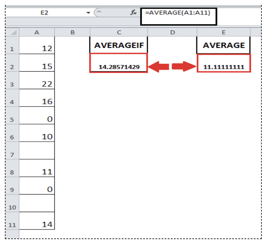
Are you still looking for help with the Average function? View our comprehensive round-up of Average function tutorials here.
Watch Video – How to Hide Zero Values in Excel + How to Remove Zero Values
In case you prefer reading over watching a video, below is the complete written tutorial.
Sometimes in Excel, you may want to hide zero values in your dataset and show these cells as blanks.
Suppose you have a dataset as shown below and you want to hide the value 0 in all these cells (or want to replace it with something such as a dash or the text ‘Not Available’).
While you can do this manually with a small dataset, you’ll need better ways when working with large datasets.
In this tutorial, I will show you multiple ways to hide zero values in Excel and one method to select and remove all the zero values from the dataset.
Important Note: When you hide a 0 in a cell using the methods shown in this tutorial, it will only hide the 0 and not remove it. While the cells may look empty, those cells still contain the 0s. And in case you use these cells (that have hidden zeroes) in any formula, these will be used in the formula.
Let’s get started and dive into each of these methods!
Automatically Hide Zero Value in Cells
Excel has an inbuilt functionality that allows you to automatically hide all the zero values for the entire worksheet.
All you have to do is uncheck a box in Excel options, and the change will be applied to the entire worksheet.
Suppose you have the sales dataset as shown below and you want to hide all the zero values and show a blank cells instead.
Below are the steps to hide zeros from all the cells in a workbook in Excel:
- Open the workbook in which you want to hide all the zeros
- Click the File tab

- Click on Options

- In the Excel Options dialog box that opens, click on the ‘Advanced’ option in the left pane

- Scroll down to the section that says ‘Display option for this worksheet’, and select the worksheet in which you want to hide the zeros.

- Uncheck the ‘Show a zero in cells that have zero value’ option

- Click Ok


The above steps would instantly hide zeros in all the cells in the selected worksheet.
This change is also applied to cells where zero is a result of a formula.
Remember that this method only hides the 0 value in the cells and doesn’t remove these. The 0 is still there, it’s just hidden.
This is the best and fastest method to hide zero values in Excel. But this is useful only if you want to hide zero values in the entire worksheet. In case you only want this to hide zero values in a specific range of cells, it’s better to use other methods covered next in this tutorial.
Hide Zero Value in Cells using Conditional Formatting
While the above method is the most convenient one, it doesn’t allow you to hide zeros only in a specific range (rather it hides zero values in the entire worksheet).
In case you only want to hide zeros for a specific dataset (or multiple datasets), you can use conditional formatting.
With conditional formatting, you can apply a specific format based on the value in the cells. So, if the value in some cells is 0, you can simply program conditional formatting to hide it (or even highlight it if you want).
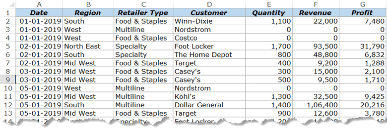
Suppose you have a dataset as shown below and you want to hide zeros in the cells.
Below are the steps to hide zeros in Excel using conditional formatting:
- Select the dataset
- Click the ‘Home’ tab

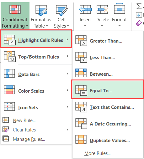
- In the ‘Styles’ group, click on ‘Conditional Formatting’.

- Place the cursor over the ‘Highlight Cells Rules’ options and in the options that show up, click on the ‘Equal to’ option.

- In the ‘Equal To’ dialog box, enter ‘0’ in the left field.

- Select the Format drop-down and click on ‘Custom Format’.

- In the ‘Format Cells’ dialog box, select the ‘Font’ tab.
- From the Color drop-down, choose the white color.

- Click OK.
- Click OK.


The above steps change the font color of the cells that have the zeros to white, which make these cells look blank.
This workaround works only when you have a white background in your worksheet. In case there is any other background-color in the cells, the white color may still keep the zeros visible.
In case you want to truly hide the zeros in the cells, where the cells look blank no matter what background color is given to the cells, you can use the steps below.
- Select the dataset
- Click the ‘Home’ tab
- In the ‘Styles’ group, click on ‘Conditional Formatting’.
- Place the cursor over the ‘Highlight Cells Rules’ options and in the options that show up, click on the ‘Equal to’ option.
- In the ‘Equal To’ dialog box, enter 0 in the left field.
- Select the Format drop-down and click on Custom Format.
- In the ‘Format Cells’ dialog box, select the ‘Number’ tab and click on the ‘Custom’ option in the left pane.
- In the Custom format option, enter the following in the Type field: ;;; (three semi-colons without space)
- Click OK.
- Click OK.

The above steps change the custom formatting of cells that have the value 0.
When you use three semi-colons as the format, it hides everything in the cell (be it numeric or text). And since this format is applied only to those cells which have the value 0 in it, it only hides the zeros and not the rest of the dataset.
You can also use this method to highlight these cells in a different color (such as red or yellow). To do this, just add another step (after Step  where you need to select the Fill tab in the ‘Format cells’ dialog box and then select the color in which you want to highlight the cells.
Both the methods covered above also work when 0 is a result of a formula in a cell.
Note: Both the method covered in this section only hide the zero values. It doesn’t remove these zeros. This means that in case you use these cells in calculations, all the zeros will be used as well.
Hide Zero Value using Custom Formatting
Another way to hide zero values from a dataset is by creating a custom format that hides the value in cells that have 0s, while any other value is displayed as expected.
Below are the steps to use a custom format to hide zeros in cells:
- Select the entire dataset for which you want to apply this format. If you want this for the entire worksheet, select all the cells
- With the cells selected, click the Home tab
- In the Cells group, click the Format option

- From the drop-down option, click on Format Cells. This will open the Format cells dialog box

- In the Format Cells dialog box, select the Number tab

- In the option on the left pane, click on the Custom option.
- In the options on the right, enter the following format in the Type field: 0;-0;;@
- Click OK


The above steps would apply a custom format to the selected cells where only those cells which have the value 0 are formatted to hide the value, while the rest of the cells display the data as expected.
How does this custom format work?
In Excel, there are four types of data formats that you specify:
- Positive numbers
- Negative numbers
- Zeros
- Text
And for each of these data types, you can specify a format.
In most cases, there is a default format – General, which keeps all these data types visible. But you have the flexibility of creating a specific format for each of these data types.
Below is the custom format structure you need to follow in case you are applying a custom format to each of these data types:
<Positive Numbers>;<Negative Numbers>;<Zeros>;<Text>
In the method covered above, I have specified the format to:
0;-0;;@
The above format does the following:
- Positive numbers are shown as is
- Negative numbers are shown with a negative sign
- Zeros are hidden (as no format is specified)
- Text is shown as is
Replace Zeros with Dash or Some Specific Text
In some cases, you may want to not just hide the zeros in the cells, but replace these with something more meaning.
For example, you may want to remove the zeros and replace it with a dash or a text such as “Not Available” or “Data Yet to Come”
This is again made possible using custom number formatting, where you can specify what a cell should display instead of a zero.
Below are the steps to convert a 0 to a dash in Excel:
- Select the entire dataset for which you want to apply this format. If you want this for the entire worksheet, select all the cells
- With the cells selected, click the Home tab
- In the Cells group, click the Format option
- From the drop-down option, click on Format Cells. This will open the Format cells dialog box
- In the Format Cells dialog box, select the Number tab
- In the option on the left pane, click on the Custom option.
- In the options on the right, enter the following format in the Type field: 0;-0;–;@

- Click OK

The above steps would keep all the other cells as is and change the cells with the value 0 to show a dash (–).
Note: In this example, I have chosen to replace the zero with a dash, but you can use any text as well. For example, if you want to show the NA in the cells, you can use the following format: 0;-0;”NA”;@
Pro Tip: You can also specify a few text colors in custom number formatting. For example, if you want the cells with zeros to show the text NA in red color, you can use the following format: 0;-0;[Red]”NA”;@
Hide Zero Values in Pivot Tables
There can be two scenarios where a Pivot Table shows the value as 0:
- The source data cells that are summarized in the Pivot Table has 0 values
- The source data cells that are summarized in the Pivot Table are blanks and the Pivot table has been formatted to show the empty cells as zero
Let’s see how to hide the zeros in the Pivot table in each scenario:
When Source Data cells have 0s
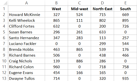
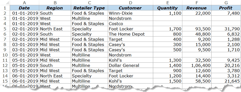
Below is a sample dataset that I have used to create a Pivot table. Note that the Quantity/Revenue/Profit numbers for all the records for ‘West’ are 0.
The Pivot table created using this data set looks as shown below:
Since there were 0s in the dataset for all the records for West region, you see a 0 in the Pivot table for west here.
If you want to hide zero in this Pivot Table, you can use conditional formatting to do this.
However, conditional formatting in the Pivot Table in Excel works a little different than regular data.
Here are the steps to apply conditional formatting to Pivot Table to hide zeros:
- Select any cell in the column that has 0s in the Pivot Table summary (Do not select all the cells, but only one cell)
- Click the Home tab
- In the ‘Styles’ group, click on ‘Conditional Formatting’.
- Place the cursor over the ‘Highlight Cells Rules’ options and in the options that show up, click on the ‘Equal to’ option.
- In the ‘Equal To’ dialog box, enter 0 in the left field.
- Select the Format drop-down and click on Custom Format.
- In the ‘Format Cells’ dialog box, select the Number tab and click on the ‘Custom’ option in the left pane.
- In the Custom format option, enter the following in the Type field: ;;; (three semi-colons without space)
- Click OK. You will see small Formatting Options icon at the right of the selected cell.
- Click on this ‘Formatting Options’ icon

- In the options that become available, choose – All cells showing “Sum of Revenue” values for “Region”.


The above steps hide the zero in the Pivot Table in such a way that if you change the Pivot Table structure (by adding more rows/columns headers to it, the zeros will continue to be hidden).
If you want to learn more about how this works, here is a detailed tutorial on the right way to apply conditional formatting to Pivot Tables.
When Source Data cells have empty cells
Below is an example where I have a dataset that has empty cells for all the records for West.
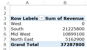
If I create a Pivot Table using this data, I will get the result as shown below.
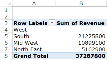
By default, the Pivot Table shows you empty cells when all the cells in the source data are blank. But in case you still see a 0 in this case, follow the below steps to hide the zero and show blank cells:
- Right-click on any of the cells in the Pivot Table
- Click on ‘Pivot Table Options’

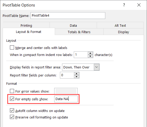
- In the ‘PivotTable Options’ dialog box, click on the ‘Layout & Format’ tab
- In the Format options, check the options and ‘For empty cells show:’ and leave it blank.

- Click OK.


The above steps would hide the zeros in the Pivot Table and show a blank cell instead.
In case you want the Pivot Table to show something instead of the 0, you can specify that in step 4. For example, if you want to show the text – ‘Data not Available’, instead of the 0, type this text in the field (as shown below).
Find and Remove Zeros in Excel
In all the methods above, I have shown you ways to hide the 0 value in the cell, but the value still remains in the cell.
In case you want to remove the zero values from the dataset (which would leave you with blank cells), use the below steps:
- Select the dataset (or the entire worksheet)
- Click the Home tab
- In the ‘Editing’ group, click on ‘Find & Select’
- In the options that are shown in the drop-down, click on ‘Replace’

- In the ‘Find and Replace’ dialog box, make the following changes:
- In the ‘Find what’ field, enter 0
- In the ‘Replace with’ field, enter nothing (leave it empty)
- Click on Options button and check the ‘Match entire cell contents’ option

- Click on Replace All


The above steps would instantly replace all the cells that had zero value with a blank.
In case you don’t want to remove the zeros right away and first select the cells, use the following steps:
- Select the dataset (or the entire worksheet)
- Click the Home tab
- In the ‘Editing’ group, click on ‘Find & Select’
- In the options that are shown in the drop-down, click on ‘Replace’
- In the ‘Find and Replace’ dialog box, make the following changes:
- In the ‘Find what’ field, enter 0
- In the ‘Replace with’ field, enter nothing (leave it empty)
- Click on Options button and check the ‘Match entire cell contents’ option
- Click on the ‘Find All’ button. This will give you a list of all the cells that have 0 in it
- Press Control-A (hold the control key and press A). This will select all the cells that have 0 in it.


Now, that you have all the cells with 0 selected, you can delete these, replace these with something else, or change the color and highlight these.
Hiding the Zeros Vs. Removing The Zeros
When treating the cells with 0s in it, you need to know the difference between hiding these and removing these.
When you hide the zero value in a cell, it is not visible to you, but it still remains in the cell. This means that if you have a dataset and you use it for calculation, that 0 value will also be used in the calculation.
On the contrary, when you have a blank cell, using it in formulas may mean that Excel automatically ignores these cells (depending on which formula you’re using).
For example, below is what I get when I use the AVERAGE formula to get the average for two columns (the result is in row 14). Column A has cells where the 0 value has been hidden (but is still there in the cell) and Column B has cells where the 0 value has been removed.
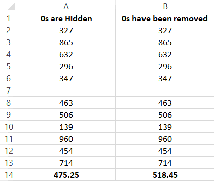
You can see the difference in the result despite the fact that the dataset for both datasets looks the same.
This happens as the AVERAGE formula ignores blank cells in column B, but it uses the ones in Column A (as the ones in column A still has the value 0 in it).
You may also like the following Excel tutorials:
- How to Hide a Worksheet in Excel
- Delete Rows Based on a Cell Value
- Delete Blank Rows in Excel
- How to Delete Every Other Row in Excel (or Every Nth Row)
- Show Formulas in Excel Instead of the Values
- Change Negative Number to Positive in Excel
- How to Remove Leading Zeros in Excel
-
#2
Assuming the range of values is in C2:C5
Try:
=COUNTIF(C2:C5,»<>0″)
-
#3
Funny.
I’m using the following formula: =COUNTIF(B57;B66;B75;B84,»<> 0″)
Excel stops and highlights B75. B57=0, B66=1, B75=1 and B84=1. Why does it not like B75? I get the error that states there is something wrong with my formula and I have the option to click OK of Help.
Thanks
-
#4
Countif only takes 2 arguments, A range and Criteria. You’ve supplied 5 arguments, 4 ranges and a criteria…
Are you trying to count every 9 rows (starting at 57) if NOT 0 ?
-
#5
If you want Excel to review the contents of cells B57, B66, B75 and B84 use:
=COUNTIF(B57,B66,B75,B84″<> 0″)
If you want it to review the two ranges B57-B66 and B75-B84 use:
=COUNTIF(B57:B66,B75:B84″<> 0″)
hope this helps
-
#6
Hmmm, so maybe COUNT is not the formula of choice.
There are 4 cells that I want to check, every 9 cells. Inbetween that range are values that do not relate to the 4 cells in question. Unless I rearrange my data. Something I want to avoid due to the vast amoutn od data that there is.
Thanks for your input.
-
#7
Try =SUM(B57<>0,B66<>0,B75<>0,B84<>0)
-
#8
Try this
=SUMPRODUCT(—(MOD(ROW(A57:A84)+6,9)=0),—(B57:B84<>0))
Counts how many are NOT 0, but only Every 9 Rows starting From row 57.
-
#9
Looks like…
=SUMPRODUCT(—(MOD(ROW(B57:B94)-ROW(B57),9)=0),—ISNUMBER(B57:B94),—(B57:B94<>0))
Hi All,
I want to COUNT the occurance that any number appears in a cell (I do not want to SUM them). How can I exclude «0» from being counted? I’d rather not leave the cell blank.
Thank you.
-
#10
Any ideas why this won’t work? =COUNTIF(G132:G6503, «<>0»)
I am using excel version 14.0.6129.5000 (32bit)