
Excel for Microsoft 365 Excel for Microsoft 365 for Mac Excel for the web Excel 2021 Excel 2021 for Mac Excel 2019 Excel 2019 for Mac Excel 2016 Excel 2016 for Mac Excel 2013 Excel 2010 Excel 2007 Excel for Mac 2011 More…Less
Multiplying and dividing in Excel is easy, but you need to create a simple formula to do it. Just remember that all formulas in Excel begin with an equal sign (=), and you can use the formula bar to create them.
Multiply numbers
Let’s say you want to figure out how much bottled water that you need for a customer conference (total attendees × 4 days × 3 bottles per day) or the reimbursement travel cost for a business trip (total miles × 0.46). There are several ways to multiply numbers.
Multiply numbers in a cell
To do this task, use the * (asterisk) arithmetic operator.
For example, if you type =5*10 in a cell, the cell displays the result, 50.
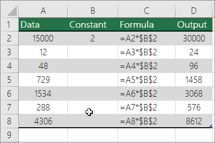
Multiply a column of numbers by a constant number
Suppose you want to multiply each cell in a column of seven numbers by a number that is contained in another cell. In this example, the number you want to multiply by is 3, contained in cell C2.
-
Type =A2*$B$2 in a new column in your spreadsheet (the above example uses column D). Be sure to include a $ symbol before B and before 2 in the formula, and press ENTER.
Note: Using $ symbols tells Excel that the reference to B2 is «absolute,» which means that when you copy the formula to another cell, the reference will always be to cell B2. If you didn’t use $ symbols in the formula and you dragged the formula down to cell B3, Excel would change the formula to =A3*C3, which wouldn’t work, because there is no value in B3.
-
Drag the formula down to the other cells in the column.
Note: In Excel 2016 for Windows, the cells are populated automatically.
Multiply numbers in different cells by using a formula
You can use the PRODUCT function to multiply numbers, cells, and ranges.
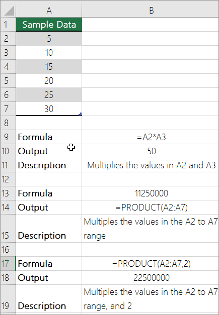
You can use any combination of up to 255 numbers or cell references in the PRODUCT function. For example, the formula =PRODUCT(A2,A4:A15,12,E3:E5,150,G4,H4:J6) multiplies two single cells (A2 and G4), two numbers (12 and 150), and three ranges (A4:A15, E3:E5, and H4:J6).
Divide numbers
Let’s say you want to find out how many person hours it took to finish a project (total project hours ÷ total people on project) or the actual miles per gallon rate for your recent cross-country trip (total miles ÷ total gallons). There are several ways to divide numbers.
Divide numbers in a cell
To do this task, use the / (forward slash) arithmetic operator.
For example, if you type =10/5 in a cell, the cell displays 2.
Important: Be sure to type an equal sign (=) in the cell before you type the numbers and the / operator; otherwise, Excel will interpret what you type as a date. For example, if you type 7/30, Excel may display 30-Jul in the cell. Or, if you type 12/36, Excel will first convert that value to 12/1/1936 and display 1-Dec in the cell.
Note: There is no DIVIDE function in Excel.
Divide numbers by using cell references
Instead of typing numbers directly in a formula, you can use cell references, such as A2 and A3, to refer to the numbers that you want to divide and divide by.
Example:
The example may be easier to understand if you copy it to a blank worksheet.
How to copy an example
-
Create a blank workbook or worksheet.
-
Select the example in the Help topic.
Note: Do not select the row or column headers.

Selecting an example from Help
-
Press CTRL+C.
-
In the worksheet, select cell A1, and press CTRL+V.
-
To switch between viewing the results and viewing the formulas that return the results, press CTRL+` (grave accent), or on the Formulas tab, click the Show Formulas button.

|
A |
B |
C |
|
|
1 |
Data |
Formula |
Description (Result) |
|
2 |
15000 |
=A2/A3 |
Divides 15000 by 12 (1250) |
|
3 |
12 |
Divide a column of numbers by a constant number
Suppose you want to divide each cell in a column of seven numbers by a number that is contained in another cell. In this example, the number you want to divide by is 3, contained in cell C2.
|
A |
B |
C |
|
|
1 |
Data |
Formula |
Constant |
|
2 |
15000 |
=A2/$C$2 |
3 |
|
3 |
12 |
=A3/$C$2 |
|
|
4 |
48 |
=A4/$C$2 |
|
|
5 |
729 |
=A5/$C$2 |
|
|
6 |
1534 |
=A6/$C$2 |
|
|
7 |
288 |
=A7/$C$2 |
|
|
8 |
4306 |
=A8/$C$2 |
-
Type =A2/$C$2 in cell B2. Be sure to include a $ symbol before C and before 2 in the formula.
-
Drag the formula in B2 down to the other cells in column B.
Note: Using $ symbols tells Excel that the reference to C2 is «absolute,» which means that when you copy the formula to another cell, the reference will always be to cell C2. If you didn’t use $ symbols in the formula and you dragged the formula down to cell B3, Excel would change the formula to =A3/C3, which wouldn’t work, because there is no value in C3.
Need more help?
You can always ask an expert in the Excel Tech Community or get support in the Answers community.
See Also
Multiply a column of numbers by the same number
Multiply by a percentage
Create a multiplication table
Calculation operators and order of operations
Need more help?
Want more options?
Explore subscription benefits, browse training courses, learn how to secure your device, and more.
Communities help you ask and answer questions, give feedback, and hear from experts with rich knowledge.
How to divide columns in Excel
- Divide two cells in the topmost row, for example: =A2/B2.
- Insert the formula in the first cell (say C2) and double-click the small green square in the lower-right corner of the cell to copy the formula down the column. Done!
Contents
- 1 How do I split a column into two in Excel?
- 2 How do I split a whole column in sheets?
- 3 How do you divide columns in sheets?
- 4 How do I split a column into multiple columns?
- 5 How do you split a column by space in Excel?
- 6 What is the shortcut to divide in Excel?
- 7 How do you divide columns in numbers?
- 8 How do you multiply on a spreadsheet?
- 9 What is division formula?
- 10 What’s another symbol for divide?
- 11 How do you divide numbers?
- 12 Can I split a cell in Excel?
- 13 How do I split text in Excel formula?
- 14 How do I split text by space in Excel?
- 15 What is short division method?
How do I split a column into two in Excel?
Turn One Data Column into Two in Excel 2016
- Select the data that needs dividing into two columns.
- On the Data tab, click the Turn to Columns button.
- Choose the Delimited option (if it isn’t already chosen) and click Next.
- Under Delimiters, choose the option that defines how you will divide the data into two columns.
How do I split a whole column in sheets?
Using the DIVIDE Formula
Click on an empty cell and type =DIVIDE(,) into the cell or the formula entry field, replacing and with the two numbers you want to divide. Note: The dividend is the number to be divided, and the divisor is the number to divide by.
How do you divide columns in sheets?
Split data into columns
- On your computer, open a spreadsheet in Google Sheets.
- At the top, click Data.
- To change which character Sheets uses to split the data, next to “Separator” click the dropdown menu.
- To fix how your columns spread out after you split your text, click the menu next to “Separator”
How do I split a column into multiple columns?
So, you can split the Sales Rep first name and last name into two columns. Select the “Sales Rep” column, and then select Home > Transform > Split Column. Select Choose the By Delimiter. Select the default Each occurrence of the delimiter option, and then select OK.
How do you split a column by space in Excel?
Click the “Data” tab in the ribbon, then look in the “Data Tools” group and click “Text to Columns.” The “Convert Text to Columns Wizard” will appear. In step 1 of the wizard, choose “Delimited” > Click [Next]. A delimiter is the symbol or space which separates the data you wish to split.
What is the shortcut to divide in Excel?
You can insert a division symbol by shortcut key in Excel. Select a cell you will insert division symbol, hold the Alt key, type 0247 and then release the Alt key. Then you can see the ÷ symbol is showing in the selected cell. Note: The number 0247 you typed must in the numeric keypad.
How do you divide columns in numbers?
Divide a column of numbers by a constant number
In this example, the number you want to divide by is 3, contained in cell C2. Type =A2/$C$2 in cell B2. Be sure to include a $ symbol before C and before 2 in the formula. Drag the formula in B2 down to the other cells in column B.
How do you multiply on a spreadsheet?
How to multiply two numbers in Excel
- In a cell, type “=”
- Click in the cell that contains the first number you want to multiply.
- Type “*”.
- Click the second cell you want to multiply.
- Press Enter.
- Set up a column of numbers you want to multiply, and then put the constant in another cell.
What is division formula?
The division formula is used for splitting a number into equal parts. Symbols that we use to indicate division are (÷) and (/). Thus, “p divided by q” can be written as: (p÷q) or (p/q).
What’s another symbol for divide?
Other symbols for division include the slash or solidus /, the colon :, and the fraction bar (the horizontal bar in a vertical fraction).
How do you divide numbers?
Divide whole numbers
Multiply the quotient by the divisor and write the product under the dividend. Subtract that product from the dividend. Bring down the next digit of the dividend. Repeat from Step 1 until there are no more digits in the dividend to bring down.
Can I split a cell in Excel?
Split cells
In the table, click the cell that you want to split. Click the Layout tab. In the Merge group, click Split Cells. In the Split Cells dialog, select the number of columns and rows that you want and then click OK.
How do I split text in Excel formula?
1st method
You can do so, click on the header ( A , B , C , etc.). Then click the little triangle and select “Insert 1 right”. Repeat to create a second free column. In the first free column, write =SPLIT(B1,”-“) , with B1 being the cell you want to split and – the character you want the cell to split on.
How do I split text by space in Excel?
Select the text you wish to split, and then click on the Data menu > Split text to columns. Select the Space.
What is short division method?
In arithmetic, short division is a division algorithm which breaks down a division problem into a series of easier steps. It is an abbreviated form of long division — whereby the products are omitted and the partial remainders are notated as superscripts.
![]()
Download Article
![]()
Download Article
This wikiHow will show you how to divide one column by another column in Microsoft Excel for Windows or macOS. In Excel, the forward-slash (/) acts as a division symbol, making it easy to divide cells with a simple formula.
-
1
Open your project in Excel. You can either open your project within Excel by navigating to File > Open or by right-clicking the file in Finder and selecting Open With > Excel.
-
2
Select the column where you want to put the division results. For example, if you want to divide column A by column B, you might select column C. Click the letter above a column to select all of its cells.
Advertisement
-
3
Type «=A1/B1» in the formula bar. Replace «A1» and «B1» with the actual cell locations you want to divide. For example, if you want to divide column A by column B and the first values appear in row 1, you’d use A1 and B1. Although you’re entering specific cells now, you’ll be applying the formula to the whole column in a moment.[1]
- The formula bar is right above the sheet.
-
4
Press Ctrl+↵ Enter (Windows) or ⌘ Cmd+⏎ Return (Mac). This applies the formula to the entire selected column so the selected column will divide A by B.[2]


Advertisement
Ask a Question
200 characters left
Include your email address to get a message when this question is answered.
Submit
Advertisement
Thanks for submitting a tip for review!
References
About This Article
Article SummaryX
1. Open your project in Excel.
2. Select the column where you want to put your division results.
3. Enter «=A1/B1» in the formula bar.
4. Press Ctrl + Enter (Windows) or Cmd + Return (Mac).
Did this summary help you?
Thanks to all authors for creating a page that has been read 24,523 times.
Is this article up to date?
See all How-To Articles
This tutorial will demonstrate how to divide cells and columns in Excel and Google Sheets.
The Divide Symbol
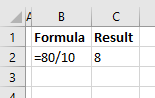
The divide symbol in Excel is the forward slash on the keyboard (/). This is the same as using the division sign (÷) in mathematics. When you divide two numbers in Excel, start with an equal sign (=), which will create a formula. Then type in the first number (the number you want to divide), followed by the forward slash, and then the number you wish to divide by.
=80/10The result of this formula would then be 8.
Divide With a Cell Reference and a Constant
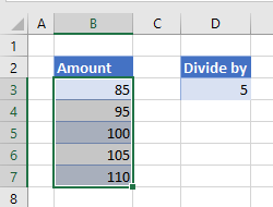
For greater flexibility in your formula, use the reference of a cell as the number to be divided and a constant as the number to divide by.
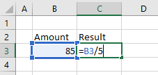
To divide B3 by 5, type the formula:
=B3/5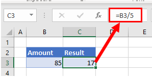
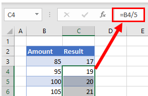
Then copy this formula down the column to the rows below. The constant number (5) will remain the same but the cell address for each row will change according to the row you are in due to Relative Cell referencing.
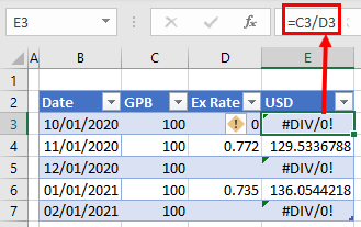
Divide a Column With Cell References
You can also use a cell reference for the number to divide by.
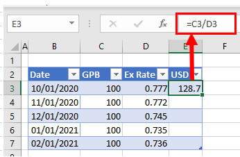
To divide cell C3 by cell D3, type the formula:
=C3/D3Since the formula uses cell addresses, you can then copy this formula down to the rest of the rows in the table.
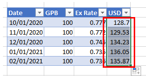
As the formula uses Relative Cell addresses, the formula will change according to the row it is copied down to.
Note: that you can also divide numbers in Excel by using the QUOTIENT Function.
Divide a Column With Paste Special
You can divide a column of numbers by a divisor, and return the result as a number within the same cell.
- Select the divisor (in this case, 5) and in the Ribbon, go to Home > Copy, or press CTRL + C.
- Highlight the cells to be divided (in this case B3:B7).
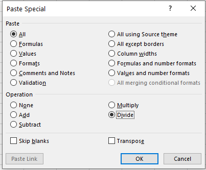
- In the Ribbon, go to Home > Paste > Paste Special.
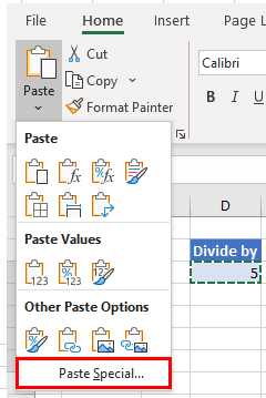
- In the Paste Special dialog box, select Divide and then click OK.
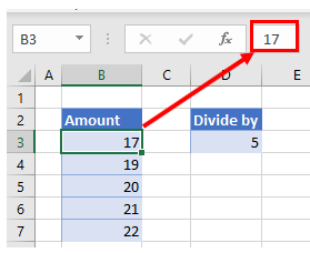
The values in the highlighted cells will be divided by the divisor that was copied and the result will be returned in the same location as the highlighted cells. In other words, you will overwrite your original values with the new divided values; cell references are not used in this this method of calculation.
The #DIV/0! Error
If you try and divide a number by zero, you will get an error as there is no answer when a number is divided by zero.
You will also get an error if you try and divide a number by a blank cell.
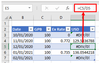
To prevent this from happening, you can use the IFERROR Function in your formula.
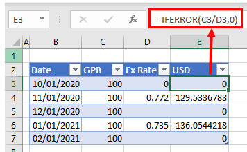
Using the methods above, you can also add, subtract, or multiply cells and columns in Excel.
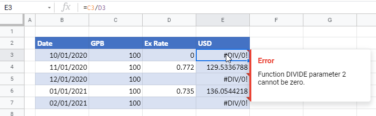
How to Divide Cells and Columns in Google Sheets
Apart from the divide Paste Special function (which does not work in Google Sheets), all of the above examples will work in exactly the same way in Google Sheets.
When working with data and spreadsheets, readability, and structure matter a lot.
It makes the data easier to skim through and work with. One of the best ways to make your data more readable is to split it into chunks so that it is easier to access the right information.
When entering data from scratch, it’s possible to ensure that we structure the data to be more readable. However, sometimes you need to work with data that someone else has created.
If the volume of the data is very large then it’s usually quite difficult to structure the data’s readability.
For example, you might have got data with a list of names, and you might want to arrange the names in alphabetical order of surnames.

In other cases, you might have got a list of addresses, but want to organize this data properly so you can clearly see how many of the people reside in, say, New York.
The best way to work through the above two problems is by splitting one column into multiple columns.
The new versions of Excel provide a special feature that lets you do that using the ‘Data’ menu.
Let’s see how this can be achieved in both the above cases.
Say you have a list of names that you want to split into columns Name and Surname.
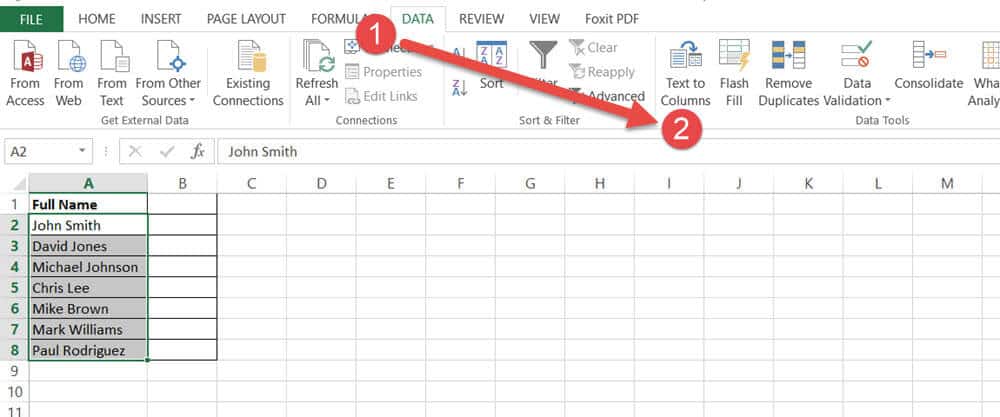
- Select the column that you want to split

- From the Data ribbon, select “Text to Columns” (in the Data Tools group). This will open the Convert Text to Columns wizard.

- Here you’ll see an option that allows you to set how you want the data in the selected cells to be delimited. Make sure this option is selected. If you’re not familiar with the term ‘delimited’, it is the character that specifies how the data in the cells are separated from each other, for example, the first name and last name in each cell are separated by a space. This means the delimiter here is a space character.

- Click Next
- Here are the settings you need to do in the second steps of the Tetx to Columns wizard:
- By default, you’ll find the Tab delimiter checked. But we don’t want to use that. We want to use Space delimiter. So uncheck the Tab delimiter and check the Space option (1).
- There is also a checkbox that lets you specify if you want to treat consecutive delimiters as one(2). That means if you have two spaces between names by mistake, do you want to treat it as one space?
- You can see how your data is going to look after the split in the data preview area (3) at the bottom of the dialog box. Notice when the space option is checked we get exactly the result we want.
- Finally Click Next (4)
- You’ll now see an option where you can specify the format for the data in the columns. By default, the General option is selected, which ensures that the columns have the same format as the original cells. Leave it with the General option selected and then click Finish.


We now have two columns of data, with the first name in Column A and last name in Column B.

It’s important to note that when you split the contents of a cell, Excel does not insert new cells to hold the contents.
So the new cells will overwrite the contents in the next cell on the right. Therefore, you should make sure that you leave an empty space on the right before splitting.
You also have the option to select the destination of the split data.
You can specify this during Step 7 by typing in the location where you want the split cells to be displayed in the destination input box. You can also select the destination cell from here.
It goes without saying that the number of columns that your data will be split into depends on the delimiters that you selected.
That means if you have a comma as a delimiter and in some cells, you have three words separated by commas then your data will be split into three columns.
How to Split Multiple Lines in a Cell into Multiple Cells
Now let’s discuss how to go about cases where you have a lot of information provided in separate lines of a cell.
Take for example the sheet below.
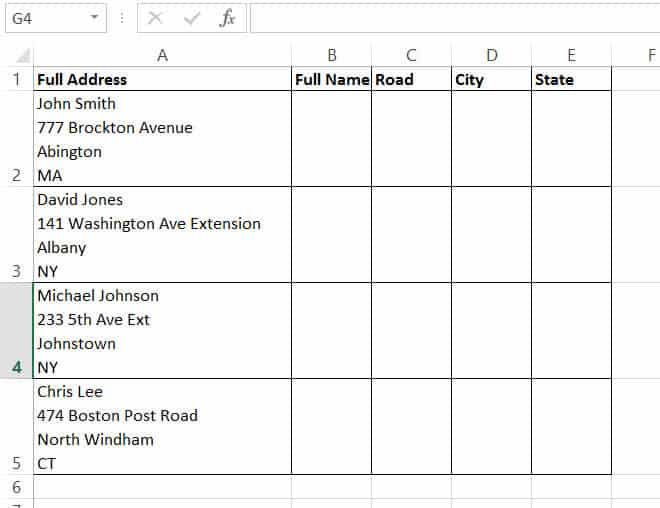
Here you can see a whole address given in each cell. Each part of the address is on a separate line of a cell. Separating this column into four different columns that can show the full name of the person, Street, City and Country would make it much easier to identify patterns in the data.
Unfortunately separating cells with multiple lines is not as easy as the method given above. But it’s not too tough either. Here’s how you can go about this problem.
- Select the column that you want to split
- From the Data ribbon, select “Text to Columns” (in the Data Tools group). This will open the Convert Text to Columns wizard.
- Here you’ll see an option that allows you to set how you want the data in the selected cells to be delimited. Make sure this option is selected.
- Click Next
- By default, you’ll find the Tab delimiter checked. Uncheck all the checked delimiters and select the ‘Other’ option. In the small box next to this option, you need to specify the delimiter character that you want to use. If you want to specify a line break character. Press Ctrl + J on your keyboard. This will show a tiny blinking dot inside the box. This means that the line break delimiter has been inserted.

You can see how your data is going to look after the split in the data preview area at the bottom of the dialog box.
Notice we get exactly the result we want. We have all the names in the first column, the second lines (Street names) in the second column, the city names in the third column, and the country names in the fourth column.
- Click Next.
- You’ll now see an option where you can specify the format for the data in the columns. By default, the General option is selected, which ensures that the columns have the same format as the original cells.
- Here we also want all the columns to appear from column B onwards so the new cells don’t overwrite the existing column. Next to Destination, we see the cell ‘$A$2’ written. We can change this by selecting our required destination cell ‘$B$2’ and then click Finish.
- You might get a dialog box asking you if you want to replace the data that is already present in the destination cells. Click on OK.


Once this is done, you will find columns B through E each containing a separate element of the address that was present in Column A.

How to Split up a Merged Cell
Before we end the article we want to add one more case. You may have more than one cells merged together and be looking for a way to unmerge or split these cells. We would like to also address this issue, in case you landed on our page looking for a solution to that. Here are the steps:
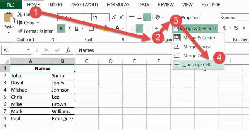
- Click on the merged cell. If there is more than one cell that you want to un-merge, select all of them.

- Under the Home Tab’s Alignment tools, you will see a drop-down next to the option that says Merge and Center. Click on the dropdown arrow and select “Unmerge Cells”.

- This will split the merged cell back to the original number of cells.

Note that Excel does not have the option to split an unmerged cell into smaller cells (as is possible in MS Word).
We have discussed how you can split cells in Excel into separate cells using different types of delimiters. We have also taken a brief look at how to split cells that had been previously merged.
The above steps have been specified assuming that you are using Excel versions 2013 to 2019. However, Microsoft keeps updating its menus, tabs, and options in every new version it brings out.
So we cannot say for sure if the methods we mentioned will work on later versions of Excel.
I hope you found this tutorial useful!
Other Excel tutorials you may find useful:
- How to Find Merged Cells in Excel
- How to Merge First and Last Name in Excel
- How to Make all Cells the Same Size in Excel (AutoFit Rows/Columns)
- How to Remove Apostrophe in Excel
- How to Remove Commas in Excel (from Numbers or Text String)
- How to Flip Data in Excel (Columns, Rows, Tables)?
- How to Convert Columns to Rows in Excel?
- How to Combine Two Columns in Excel (with Space/Comma)
Introduction to Divide in Excel
In Excel, the division is an arithmetic operation commonly used to divide numbers or values of the cell. It is one of the basic mathematical functions essential for solving complex numeric problems. Unlike addition, which has built-in functions such as the SUM function, no such function is available for division in Excel. To divide numbers or values of a cell in Excel, you need to start with an equal sign (=), followed by the numbers you want to divide, and put a forward slash (/) between the numbers.
Businesses often use the divide formula in Excel to calculate and perform various financial and work management tasks. For instance, they might calculate profit margins, monthly budgets, employee wages, expenditure reports, and other important metrics.
Let’s start by understanding how you can perform division in Excel.
Divide Formula in Excel
The arithmetic operation or formula for division in Excel starts with an equal sign (=) followed by entering the values or cell references you want to divide and a forward slash (/) between them.
![]()
How to Divide Numbers in a Cell in Excel?
To divide numbers in a cell, directly type the numbers within the cell and apply the divide formula. For example, if you want to divide 10 by 5, enter “=10/5” in a cell and press “Enter”. The division formula “=10/5” will give a result of 2.
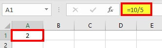
Note: Please start the formula with an equal sign (=) and use the (/) operator between two values in each cell to get the output. Or else Excel will consider the equation as a date. For instance, If you only type 10/5 in a cell, Excel will display 05-Oct.
Example #1
You can download this Divide Formula Excel Template here – Divide Formula Excel Template
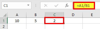
How to Divide Numbers Using Cell References?
You can divide the numbers of two cells by specifying the cell references in the divide formula.
For example, we want to divide the Cell A1 value by the Cell B1 value and display the result in Cell C1.
Solution:
Enter the formula “=A1/B1” in Cell C1 and press “Enter”, where the Cell A1 value is the dividend and Cell B2 value is the divisor. The result will be displayed in Cell C1.
Example #2
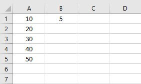
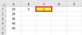
How to Divide a Column of Numbers by a Constant Number?
Suppose you want to divide the value of each cell of a column by a certain number obtained in another cell. You can easily do this task. In the below example, you will learn how to divide the values of column A by the value of Cell B1.
Solution:
Step 1: Click on Cell C1
Step 2: Enter the formula =”A1/$B$1” and press “Enter”.
Note: The symbol $ in Excel is used for absolute cell references. If you place a dollar sign ($) in front of a row, that row is fixed, and if you place a dollar sign ($) in front of a column, that column is fixed. In the formula =”A1/$B$1”, the value of the divisor is constant as the value of Cell B1.
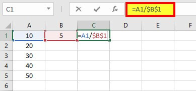
Result 2 is displayed in cell C1.
Step 3: Now, drag the cell with the formula to get the desired output.
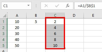
Congratulations, you have successfully done this task.
Example #3
How to Divide Columns in Excel?
You can divide column 1 with column 2 by using the division formula. Consider the below table with numbers in columns A and B. Follow the below steps to learn how to divide two columns in Excel.
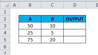
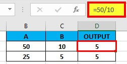
Solution:
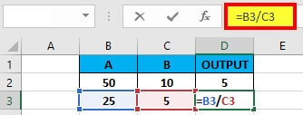
Step 1: Click on the Cell D3.
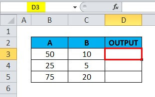
Step 2: Enter the formula “=B3/C3” in Cell D3, as shown below.
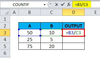
Result 5 is displayed in Cell D3.
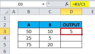
Step 3: Drag the formula on the corresponding cell to get the following output.
Example #4
How to Use the Division (/) Operator with Subtraction Operators (-) in Excel?
Under this method, you will learn to use division operators with other arithmetic operators like subtraction to solve complex division problems.
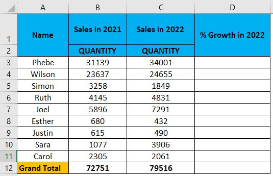
For example, you have the below data of salespersons and their actual sales in 2021 and 2022. You have to calculate the sales growth percentage for the respective salesperson in 2022. Here, you have to use the division formula along with the subtraction and percentage operator.
Solution:
Step 1: Click on the Cell D3
Step 2: Enter the formula “=(C3-B3)/B3” in Cell D3
Note: Using this formula, “=(C3-B3)/B3”, you can calculate the sales growth percentage for the respective salesperson.
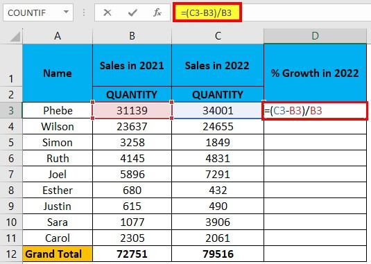
The output is 9%.
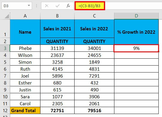
Note: The answer to the formula “=(C3-B3)/B3” is 0.091910466. For converting the decimal value into a percentage, select Cell D3, go to the “Home” tab, and click “Percentage” in the Number section. The result is 9%, as shown in the above image.
Step 3: Drag the cell with the formula downwards to get the desired output
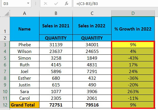
The above result shows the sales growth percentage for the individual salesperson.
Example # 5
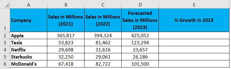
We have the sales data for five famous companies (Apple, Tesla, Netflix, Starbucks, and McDonald’s) for 2021 and 2022 and the estimated figures for 2023. We need to calculate the percentage growth rate for each company for 2023 using basic mathematical operators such as division, subtraction, and the percentage operator.
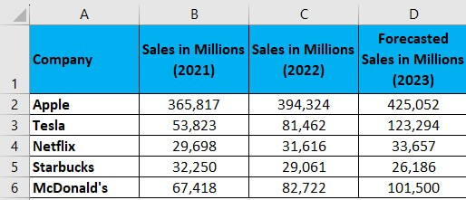
Solution:
Step 1: Add the title “% Growth in 2023” to column E, as shown below.
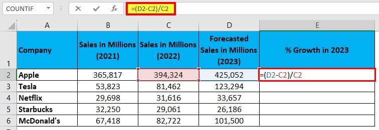
Step 2: Click on Cell E2.
Step 3: Enter the formula “=(D2-C2)/C2”, as shown below.
According to this formula, we will subtract the sales value of 2022 from 2023 and then divide the result by the sales value of 2022. The output is the percentage increase in sales from 2022 to 2023.
Note: In this example, we used the formula’s opening and closing parenthesis, “( )”.
The output is 8%, as shown below.
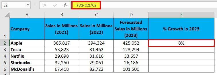
Note: The formula “=(B2+C2)/D2” will give a decimal value. Thus, convert this decimal value into %.
Step 4: Now, drag the cell with the formula to get the result, as shown below.
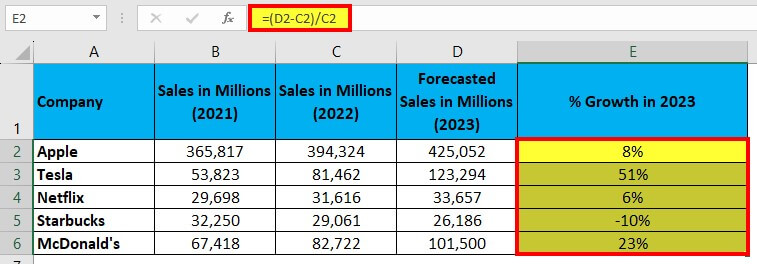
The future sales growth in percentage for all five companies in 2023 is now ready.
How to Use the Division Operator (/) with Addition (+)?
Under this method, you will learn to use the division operator with the addition operator (+) with the help of the following examples.
Example #6
Using Nested Parentheses in Division Operator Using Addition (+)
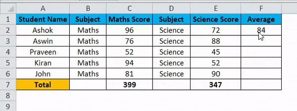
In this example, we will calculate the average of the student’s marks in maths and science by using the division and addition operator.
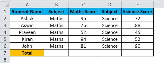
The formula for calculating the average marks of students is:“Total Number of Marks Scored / Number of Subjects.
Solution:
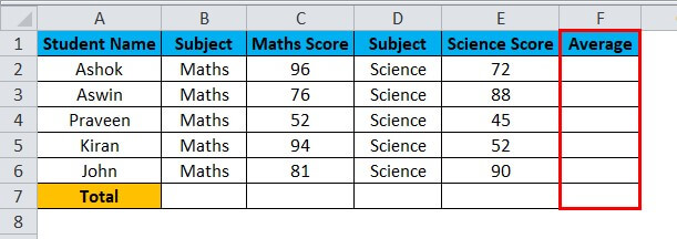
Step 1: Add a new column, “Average”, as shown below.
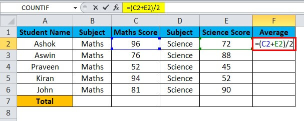
Step 2: Enter the formula “=(C2+E2)/2” in Cell F2.
The formula states to add the marks of Maths and Science subjects and then divide by the total subject, i.e., 2.
Result 84 is displayed, as shown in the below image.
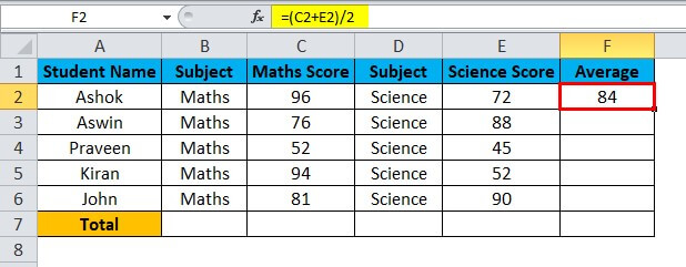
Step 3: Now, drag the cell with the formula to the rest of the cells.
The average score of the students in Maths and Science subjects is displayed.
How to Handle #DIV/0! Error Using IF Function?
While executing the division operation on a data set, Excel will display the error of #DIV/0! when the formula tries to divide a number by an empty cell or 0. In the following example, you will learn how to use the IF function, such as the “IFERROR” condition, to prevent and resolve the #DIV/0! Error.
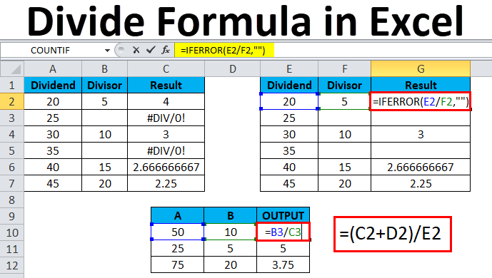
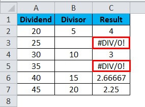
Suppose you have the below table of dividends and divisors. You have applied the division formula to this data, and Excel has shown error #DIV/0! in Cell C3 and Cell C5 because Cell B3 and Cell B5 have no value. Now, you want to overcome this problem.
Solution:
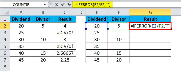
Step 1: Click Cell G2 of the Result column.
Step 2: Enter the IFERROR formula “=IFERROR(E2/F2,””)” as shown below and press “Enter”.
Note: The Formula “=IFERROR(E2/F2,””)” indicates that divide the value of Cell E2 by Cell F2, and if there is an empty cell or 0 value, then leave the cell blank in the result column to avoid displaying of the #DIV/0! Error.
Output 4 is displayed.
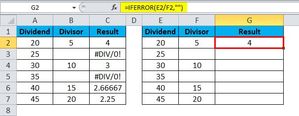
Step 3: Drag the cell with the formula as shown below.
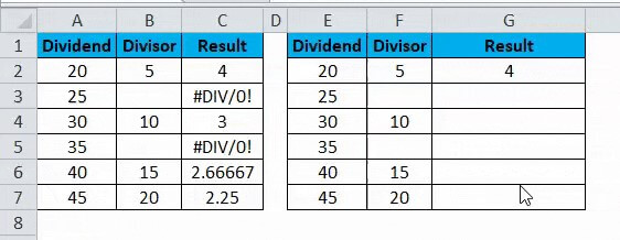
The result is displayed above, and Cell G3 and Cell G5 are blank instead of #DIV/0! Error.
Things to Remember while Using the Divide Function in Excel
- Put an equal sign (=) in the cell before using the divide formula.
- While selecting the data for calculation, do not select the row or column headers.
- If there is an empty cell or 0 value in the Cell, then Excel will throw an #DIV/0!
- You should properly use the opening and closing parenthesis in the division formula. For example, formulas like “=10/4-2” will give 0.5 output, and “=10/(4-2)” will give 5 output. Always remember, the “PEDMAS” is the order of calculations in Excel.
- If you want to display only the integer value of a division operation, use the QUOTIENT function of Excel.
Frequently Asked Questions (FAQS)
Q1. What is the symbol for the divide in Excel?
Answer: The symbol or arithmetic operator used to represent divide or division in Microsoft Excel is “/”, a forward slash. The Excel division formula is “=x/y,” where x is the dividend and y is the divisor.
Q2. How to divide in Excel?
Answer: There are various methods to divide in Excel. You can directly type the numbers in a cell or divide two (or more) numbers by referring to a cell or constant number. As seen in the image below, you must use an equal sign (=) before the division formula and a forward slash (/) between the numbers or cells you want to divide.
Q3. What is the other method for division in Excel?
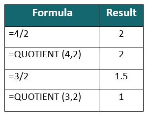
Answer: The alternate method for dividing numbers is using the “QUOTIENT” formula. When you want to display only the integer part of a division, use the formula “QUOTIENT(numerator, denominator)”. If a division equation has a remainder value, the QUOTIENT function will only return the integer value as an output. For example,” =3/2” returns 1.5 whereas “=QUOTIENT(3,2)” returns 1, where 1.5 is the remainder, and 1 is the integer/quotient.
Recommended Articles
This article has been a guide to Dividing in Excel. Here we discuss the Divide Formula in Excel and How to use Divide Formula in various scenarios using practical examples. You also get a downloadable Excel template for your reference. Furthermore, you can read our other suggested articles.
- Divide Cell in Excel
- Formatting Text in Excel
- Statistics in Excel
- Carriage Return in Excel
In Excel, you can divide in a cell, cells, columns of cells, a range of cells by a constant number, and by using the QUOTIENT function.

In Excel, you can divide within a cell, cell by cell, columns of cells, range of cells by a constant number, and divide using QUOTIENT function.
Dividing using Divide symbol in a cell
The easiest method to divide numbers in excel is by using the divide operator. In MS Excel, the divide operator is a forward slash (/).
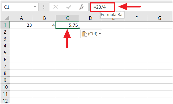
To divide numbers in a cell, simply, start a formula with the ‘=’ sign in a cell, then enter the dividend, followed by a forward slash, followed by the divisor.
=number/numberFor example, to divide 23 by 4, you type this formula in a cell: =23/4
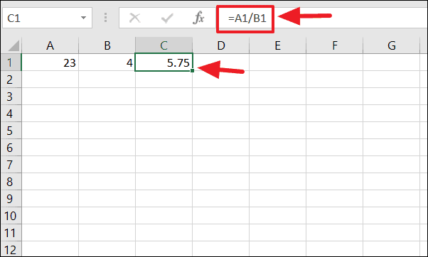
Dividing Cells in Excel
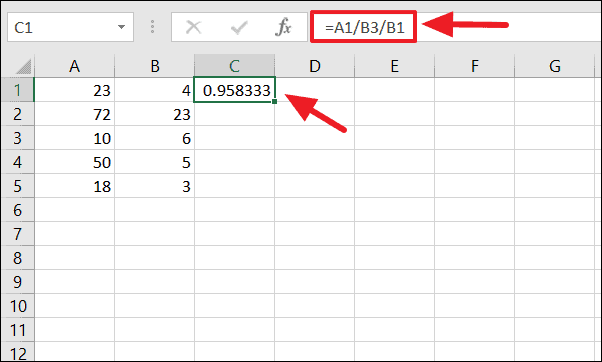
To divide two cells in Excel, enter the equals sign (=) in a cell, followed by two cell references with the division symbol in between. For example, to divide the cell value A1 by B1, type ‘=A1/B1’ in cell C1.
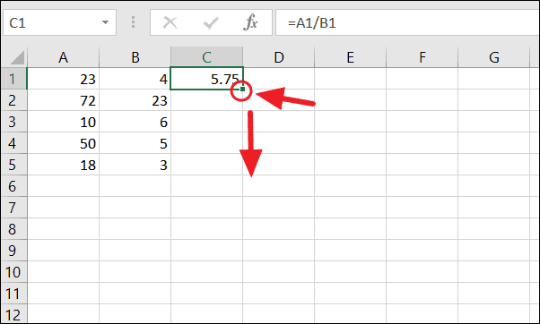
Dividing Columns of Cells in Excel
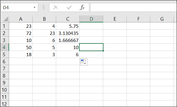
To divide two columns of numbers in Excel, you can use the same formula. After you, typed the formula in the first cell (C1 in our case), click on the small green square in the lower-right corner of cell C1 and drag it down to cell C5.
Now, the formula is copied from C1 to C5 of column C. And column A is divided by column B, and the answers were populated in column C.
For example, to divide the number in A1 by the number in B2, and then divide the result by the number in B1, use the formula in the following image.
Dividing a Range of Cells by a Constant Number in Excel
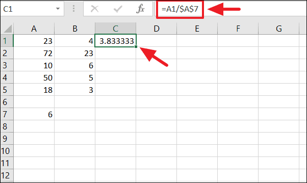
If you want to divide a range of cells in a column by a constant number, you can do that by fixing the reference to the cell that contains the constant number by adding the dollar ‘$’ symbol in front of the column and row in the cell reference. This way, you can lock that cell reference so it won’t change no matter where the formula is copied.
For example, we created an absolute cell reference by placing a $ symbol in front of the column letter and row number of cell A7 ($A$7). First, enter the formula in cell C1 to divide the value of cell A1 by the value of cell A7.
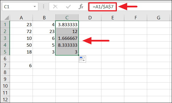
To divide a range of cells by a constant number, click on the small green square in the lower-right corner of cell C1 and drag it down to cell C5. Now, the formula is applied to C1:C5 and cell C7 is divided by a range of cells (A1:A5).
Divide a Column by the Constant Number with Paste Special
You can also divide a range of cells by the same number with Paste Special method. To do that, right-click on the cell A7 and copy (or press CTRL + c).
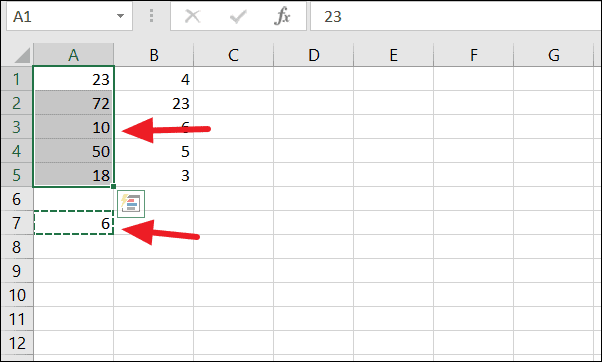
Next, select the cell range A1:A5 and then right-click, and click ‘Paste Special’.
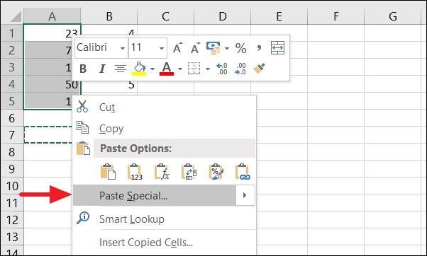
Select ‘Divide’ under ‘Operations’ and click the ‘OK’ button.
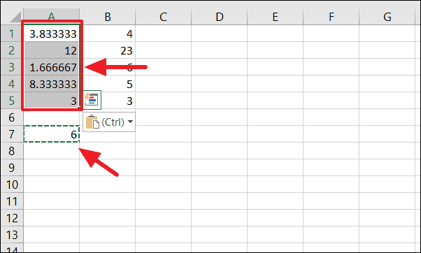
Now, cell A7 is divided by the column of numbers (A1:A5). But the original cell values of A1:A5 will be replaced with the results.
Dividing in Excel using QUOTIENT Function
Another way to divide in Excel is by using the QUOTIENT function. However, dividing numbers of cells using the QUOTIENT returns only the integer number of a division. This function discards the remainder of a division.
The Syntax for QUOTIENT function:
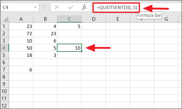
=QUOTIENT(numerator, denominator)When you divide two numbers evenly without remainder, the QUOTIENT function returns the same output as the division operator.
For example, both =50/5 and =QUOTIENT(50, 5) yields 10.
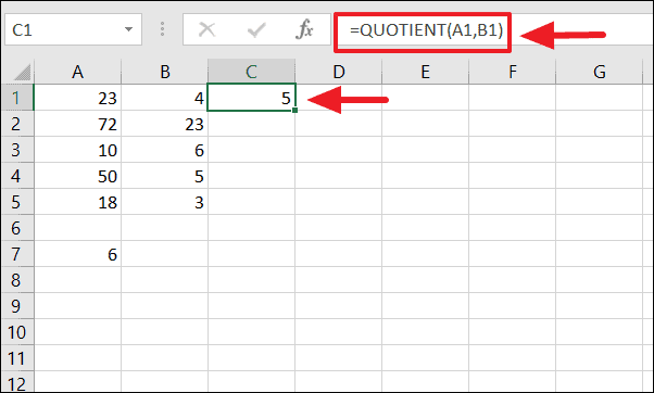
But, when you divide two numbers with a remainder, the divide symbol produces a decimal number while the QUOTIENT returns only the integer part of the number.
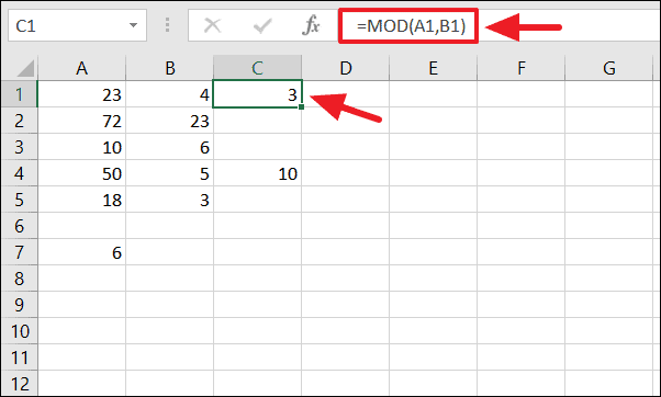
For example, =A1/B1 returns 5.75 and =QUOTIENT(A1,B1) returns 5.
If you only want the remainder of a division, not an integer, then use the Excel MOD function.
For example, =MOD(A1,B1) or =MOD(23/4) returns 3.
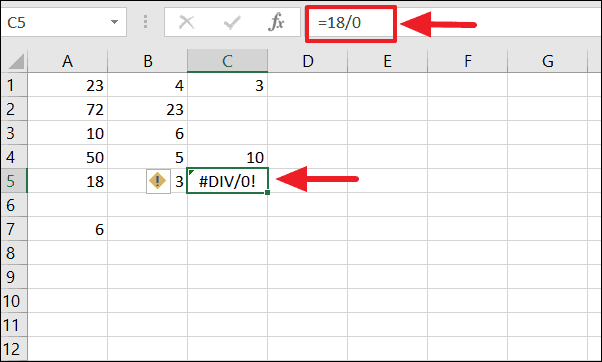
#DIV/O! Error
#DIV/O! error value is one of the most common errors associated with division operations in Excel. This error will be displayed when the denominator is 0 or the cell reference is incorrect.
We hope this post helps you divide in Excel.
Do you have any tricks on how to split columns in excel? When working with Excel, you may need to split grouped data into multiple columns. For instance, you might need to separate the first and last names into separate columns.
With Excel’s “Text to Feature” there are two simple ways of splitting your columns. If there is an evident delimiter such as a comma, use the “Delimited” option. However, the “Fixed method is ideal for splitting the columns manually.”
To learn how to split a column in excel and make your worksheet easy-to-read, follow these simple steps. You can also check our Microsoft Office Excel Cheat Sheet here. But, first, why should you split columns in excel?
Jump to:
- Why you need to split cells
- How do you split a column in excel?
- Method 1- Delimited Option
- Method 2- Fixed Width
- How to Split One Column into Multiple Columns in Excel
- Method 3- Split Columns by Flash Fill
- Method 4- Use LEFT, MID and RIGHT text string functions
Why you need to split cells
If you downloaded a file that Excel can’t divide, then you need to separate your columns. You should split a column in excel if you want to divide it with a specific character. Some examples of familiar characters are commas, colons, and semicolons.
How do you split a column in excel?
Method 1- Delimited Option
This option works best if your data contains characters such as commas or tabs. Excel only splits data when it senses specific characters such as commas, tabs, or spaces. If you have a Name column, you can separate it into First and Last name columns
- First, open the spreadsheet that you want to split a column in excel
- Next, highlight the cells to be divided. Hold the SHIFT key and click the last cell on the range
- Alternatively, right-click and drag your mouse to highlight the cells
- Now, click the Data tab on your spreadsheet.
- Navigate to and click on the “Text to Columns” From the Convert Text to Columns Wizard dialog box, select Delimited and click “Next.”
- Choose your preferred delimiter from the options given and click “Next.”
- Now, highlight General as your Column Data Format
- “General” format converts all your numeric values to numbers. Date values are converted to dates, and the rest of the data is converted to text. “Text” format only converts the data into text. “Date” allows you to select your desired date format. You can skip the column by choosing “Do not import column.”
- Afterward, type the “Destination” field for your new column. Otherwise, Excel will replace the initial data with the divided data
- Click “Finish” to split your cells into two separate columns.
Method 2- Fixed Width
This option is ideal if spaces separate your column data fields. So, Excel splits your data based on the character counts, be it 5th or 10th characters.
- Open your spreadsheet and select the column you wish to split. Otherwise, the “Text Columns” will be inactive.
- Next, click Text Columns in the “Data” Tab
- Click Fixed Width and then Next
- Now you can adjust your column breaks in the “Data preview.” Unlike the “Delimited” option that focuses on characters, in “Fixed Width,” you select the position of splitting the text.
- Tips: Click the preferred position to CREATE a line break. Double-Click on the line to delete it. Click and drag a column break to move it
- Click Next if you’re satisfied with the results
- Select your preferred Column Data Format
- Next, type the “Destination” field for your new column. Otherwise, Excel will replace the initial data with the divided data.
- Finally, click Finish to confirm the changes and divide your column into two
How to Split One Column into Multiple Columns in Excel
A single column can be split into multiple columns using the same steps outlined in this guide
Tip: The number of columns depends on the number of delimiters that you select. For instance, Data will be split into three columns if it contains three commas.
Method 3- Split Columns by Flash Fill
If you are using Excel 2013 and 2016, you are in luck. These versions are integrated with a Flash fill feature that extracts data automatically once it recognizes a pattern. You can use flash fill to split the first and last name in your column. Alternatively, this feature combines separate columns into one column.
If you don’t have these professional versions, quickly upgrade your Excel version. Follow these steps to divide your columns using Flash Fill.
- Assume your data resembles the one in the image below

- Next, in cell B2, type the First Name as below

- Navigate to the Data Tab and click Flash Fill. Alternatively, use the shortcut CTRL+E
- Selecting this option automatically separates all the First Names from the given column
Tip: Before clicking Flash Fill, ensure that cell B2 is selected. Otherwise, a warning appears that
- Flash Fill cannot recognize a pattern to extract the values. Your extracted values will look like this:

- Apply the same steps for the last name as well.

Now, you have learned to split a column in excel into multiple cells
Method 4- Use LEFT, MID and RIGHT text string functions
Alternatively, use LEFT, MID, and RIGHT string functions to split your columns in Excel 2010, 2013 and 2016.
- LEFT function: Returns the first character or characters on your left, depending on the specific number of characters you require.
- MID Function: Returns the middle number of characters from string text beginning from where you specify.
- RIGHT Function: Gives the last character or characters from your text field, depending on the specified number of characters on your right.
However, this option is not valid if your data contains a formula such as VLOOKUP. In this example, you’ll learn how to split Address, City, and zip code columns.

To extract the Addresses using the LEFT function:
- First select cell B2
- Next, apply the formula =LEFT(A2,4)
Tip: 4 represents the number of characters representing the address
3. Click, hold and drag down the cell to copy the formula to the entire column

To extract the City data, use the MID function as follows:
- First, Select cell C2
- Now, apply the formula =MID(A2,5,2)
Tip: 5 represents the fifth character. 2 is the number of characters representing the city.
- Right-click and drag down the cell to copy the formula in the rest of the column
Finally, to extract the last characters in your data, use the Right text function as follows:
- Select Cell D2
- Next, apply the formula =RIGHT(A2,5)
Tip: 5 represents the number of characters representing the Zip Code
- Click, hold and drag down the cell to copy the formula in the entire column

Tips to remember
- The shortcut key for Flash Fill is CTRL+E
- Always try to identify a shared value in your column before splitting it
- Familiar characters when splitting columns include commas, tabs, semicolons, and spaces.
Text Columns is the best feature to split a column in excel. It might take you several attempts to master the process. But once you get the hang of it, it will only take you a couple of seconds to split your columns. The results are professional, clean, and eye-catching columns.
If you’re looking for a software company you can trust for its integrity and honest business practices, look no further than SoftwareKeep. We are a Microsoft Certified Partner and a BBB Accredited Business that cares about bringing our customers a reliable, satisfying experience on the software products they need. We will be with you before, during, and after all the sales.
Microsoft Excel is a widely used Microsoft Office application. It helps you to manage and analyze data in a spreadsheet format. More often than not, you are required to maintain large sets of data that become hard to handle. However, Excel helps you overcome this problem by providing a wide range of shortcuts and formulas. You can easily add, subtract, multiply and divide numbers in Excel.
In this article, I will help you to learn one of the arithmetic functions of Excel, that is, Division. I will focus on the different ways you can divide numbers in Excel. You will learn how to divide numbers in a cell, columns, rows, and also some additional formulas.
But before we go ahead, there are certain rules that have to be followed while applying ANY arithmetic formula in Excel.
Points to Remember When you Divide Numbers in Excel
- Always start your formula with an equal sign (=). This is a very important step because, without the equal sign, Excel would not recognize it as a formula.
Say you want to divide and you put the formula as 25/5, then Excel would consider it as a date and not a formula. So if you want to divide 25 by 5, you must use the formula as =25/5
- The next thing to focus on while writing the formula is that there should be no space in it. So if you are diving number 10 by 2, you cannot write the formula as = 10 / 2. It has to be =10/2
- Always remember the order of operations Exel uses in an arithmetic formula. You can remember the order by the acronym PEMDAS: Parenthesis, Exponentiation, Multiplication, Division, Addition, Subtraction). You can easily understand this by the example given below

Division Symbol in Excel
When you are manually doing division, you use the obelus symbol (÷). However, in Excel, you have to use the forward-slash (/) as the division symbol.
So you have to use a simple formula of =a/b for division, where :
a = dividend (the number you want to divide)
b = divisor (the number by which you want to divide the dividend)
Now that we have learned about the different rules and the symbol of division, let us dive into the article and learn about the different ways you can divide numbers in Excel.
How to Divide Numbers in a Single Cell?
This is the simplest and most common way to divide in Excel. All you have to do is write the formula in the cell where you want the answer.
Also, read How to Copy Conditional Formatting in Microsoft Excel
To perform this function you have to follow the following steps:
- Select the cell where you want to perform the division formula.
- Start by typing the equal sign (=)
- Then write the number you want to divide (dividend) and then put a forward slash (/)
- After that write the number you want your dividend to be divided by (divisor).
Here I’ve taken 100 divided by 20. So I will type =100/20

How to Divide Cells in Excel?
To divide two or more cells, you need to use the same division formula, but instead of the numbers, you have to use the cell reference.
For instance:
- To divide the cell A2 by 10, you will use the formula =A2/2

- To divide the cell A2 by cell A3, you will use the formula =A2/A3

- Lastly, if you want to divide multiple cells, all you have to do is type the cell references separated by the division symbol. So, if you wish to divide A2 by A3 and then divide its result by A4, you have to use the formula =A2/A3/A4

How to Divide Columns in Excel?
To divide columns in Excel is a pretty easy task. All you have to do is apply the division formula in the topmost cell and then copy it vertically.
To divide columns in Excel you have to follow the following steps:
- Start by selecting the top cell and apply the division formula to it.
Here I’ve taken Cell C2, where I want the result for A2/B2. So I will type the formula as =A2/B2.
- Now, you have to drag the little square at the left bottom of cell C2 vertically.

- Press enter and you have your result.

How to Divide a Column by a Constant Number?
This can be done in two ways. Now that you have learned how to divide two columns, this becomes easy to perform. Let us dive straight into it.
The first way to do it is by selecting the topmost cell in the column where you want results (say C2). Here you will type the formula as =A2/5 (assuming that you want to divide the column A by constant number 5). Now simply drag the little square and you will have your result.


To perform this function in a second way, you have to follow these steps:
- Type the constant number (divisor) in a separate cell. Here I have typed the number 5 in cell B2.
- Now in the column, you want the results, select the topmost cell (say C2) and type the formula as =A2/$B$2

- Press enter and you will have your result in the given cell. Now, all you have to do is drag the little box vertically, and you will get the result.

Note: Remember to put the cell reference in Divisor’s place in the formula. If you put the value of the cell, then the result would be the same for each cell when you drag it. You can see the example below.
Here I’ve put the value 100 in the formula instead of the cell reference of A2. So what happens now is that when you copy down the formula, each cell would show the result as 20 because each cell shows the result for the formula =100/5

How to Divide Rows in Excel?
This one becomes quite easy if you already know how to divide columns. You have to follow the same steps as dividing columns to divide rows.
Select the Left most cell in the row and apply the division formula to it. Now drag the little box horizontally and you will have your result.
You can have a look at the screenshot to understand this in a better way

How to Divide Using the QUOTIENT Function in Excel?
To understand this function, you first need to understand what a quotient is. It is the final number you get when you divide a number. It is the integer portion of the division. It discards the remainder.
The formula for using the Quotient function is =QUOTIENT (numerator, denominator)
Where:
Numerator= Dividend
Denominator= Divisor
Now you need to remember that when two numbers divide evenly without leaving any remainder, the QUOTIENT function and the simple divide method give the same result.
For instance, I want to divide 10 by 5
So I can do it in two ways,
- =10/5
- QUOTIENT(10,5)
Both of these formulas will give me the same result as 20.
However, when the two numbers do not divide evenly and leave remainder after division, the QUOTIENT function gives the answer as the integer part and leaves out the remainder. Whereas the divide method shows the answer in decimals.
For instance, I want to divide 5 by 4
- =5/4 will show the result as 1.25
- =QUOTIENT(5,4) shows the result as 1

How to Divide Using the MOD Function in Excel?
The MOD function in Excel gives you the remainder of the division. Just like the QUOTIENT function which gives you the integer after the division.
When you divide two numbers that do not divide evenly, the MOD function gives you the remainder left after division.
For Instance,
If I have to divide two numbers, say 1250 by 7. Then using the MOD function, i.e, =MOD (dividend, divisor), I will get the result as 4.
Here 4 is the remainder left after dividing 1250 and 7.

Important: the MOD function and the QUOTIENT function often show different results, even though both are dividing the given two numbers. So if I take the above example and divide 1250 by 7 using the QUOTIENT function, I will get a different answer.

You are all set to Divide in Excel!
I have covered each and every method you can use to divide in Excel. Now you can save your time by easily applying the formulas whenever you need to divide numbers in an Excel Sheet.
Go grab your laptop and give these features a try!