
Excel for Microsoft 365 Excel for Microsoft 365 for Mac Excel for the web Excel 2021 Excel 2021 for Mac Excel 2019 Excel 2019 for Mac Excel 2016 Excel 2016 for Mac Excel 2013 Excel 2010 Excel 2007 Excel for Mac 2011 More…Less
Multiplying and dividing in Excel is easy, but you need to create a simple formula to do it. Just remember that all formulas in Excel begin with an equal sign (=), and you can use the formula bar to create them.
Multiply numbers
Let’s say you want to figure out how much bottled water that you need for a customer conference (total attendees × 4 days × 3 bottles per day) or the reimbursement travel cost for a business trip (total miles × 0.46). There are several ways to multiply numbers.
Multiply numbers in a cell
To do this task, use the * (asterisk) arithmetic operator.
For example, if you type =5*10 in a cell, the cell displays the result, 50.
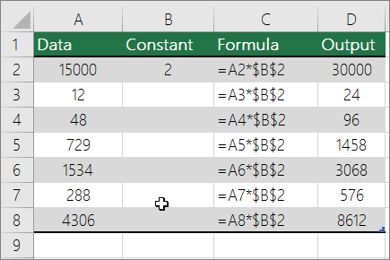
Multiply a column of numbers by a constant number
Suppose you want to multiply each cell in a column of seven numbers by a number that is contained in another cell. In this example, the number you want to multiply by is 3, contained in cell C2.
-
Type =A2*$B$2 in a new column in your spreadsheet (the above example uses column D). Be sure to include a $ symbol before B and before 2 in the formula, and press ENTER.
Note: Using $ symbols tells Excel that the reference to B2 is «absolute,» which means that when you copy the formula to another cell, the reference will always be to cell B2. If you didn’t use $ symbols in the formula and you dragged the formula down to cell B3, Excel would change the formula to =A3*C3, which wouldn’t work, because there is no value in B3.
-
Drag the formula down to the other cells in the column.
Note: In Excel 2016 for Windows, the cells are populated automatically.
Multiply numbers in different cells by using a formula
You can use the PRODUCT function to multiply numbers, cells, and ranges.
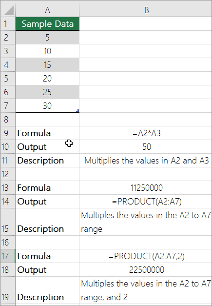
You can use any combination of up to 255 numbers or cell references in the PRODUCT function. For example, the formula =PRODUCT(A2,A4:A15,12,E3:E5,150,G4,H4:J6) multiplies two single cells (A2 and G4), two numbers (12 and 150), and three ranges (A4:A15, E3:E5, and H4:J6).
Divide numbers
Let’s say you want to find out how many person hours it took to finish a project (total project hours ÷ total people on project) or the actual miles per gallon rate for your recent cross-country trip (total miles ÷ total gallons). There are several ways to divide numbers.
Divide numbers in a cell
To do this task, use the / (forward slash) arithmetic operator.
For example, if you type =10/5 in a cell, the cell displays 2.
Important: Be sure to type an equal sign (=) in the cell before you type the numbers and the / operator; otherwise, Excel will interpret what you type as a date. For example, if you type 7/30, Excel may display 30-Jul in the cell. Or, if you type 12/36, Excel will first convert that value to 12/1/1936 and display 1-Dec in the cell.
Note: There is no DIVIDE function in Excel.
Divide numbers by using cell references
Instead of typing numbers directly in a formula, you can use cell references, such as A2 and A3, to refer to the numbers that you want to divide and divide by.
Example:
The example may be easier to understand if you copy it to a blank worksheet.
How to copy an example
-
Create a blank workbook or worksheet.
-
Select the example in the Help topic.
Note: Do not select the row or column headers.

Selecting an example from Help
-
Press CTRL+C.
-
In the worksheet, select cell A1, and press CTRL+V.
-
To switch between viewing the results and viewing the formulas that return the results, press CTRL+` (grave accent), or on the Formulas tab, click the Show Formulas button.
|
A |
B |
C |
|
|
1 |
Data |
Formula |
Description (Result) |
|
2 |
15000 |
=A2/A3 |
Divides 15000 by 12 (1250) |
|
3 |
12 |
Divide a column of numbers by a constant number
Suppose you want to divide each cell in a column of seven numbers by a number that is contained in another cell. In this example, the number you want to divide by is 3, contained in cell C2.
|
A |
B |
C |
|
|
1 |
Data |
Formula |
Constant |
|
2 |
15000 |
=A2/$C$2 |
3 |
|
3 |
12 |
=A3/$C$2 |
|
|
4 |
48 |
=A4/$C$2 |
|
|
5 |
729 |
=A5/$C$2 |
|
|
6 |
1534 |
=A6/$C$2 |
|
|
7 |
288 |
=A7/$C$2 |
|
|
8 |
4306 |
=A8/$C$2 |
-
Type =A2/$C$2 in cell B2. Be sure to include a $ symbol before C and before 2 in the formula.
-
Drag the formula in B2 down to the other cells in column B.
Note: Using $ symbols tells Excel that the reference to C2 is «absolute,» which means that when you copy the formula to another cell, the reference will always be to cell C2. If you didn’t use $ symbols in the formula and you dragged the formula down to cell B3, Excel would change the formula to =A3/C3, which wouldn’t work, because there is no value in C3.
Need more help?
You can always ask an expert in the Excel Tech Community or get support in the Answers community.
See Also
Multiply a column of numbers by the same number
Multiply by a percentage
Create a multiplication table
Calculation operators and order of operations
Need more help?
OBJECTS
Worksheets: The Worksheets object represents all of the worksheets in a workbook, excluding chart sheets.
Range: The Range object is a representation of a single cell or a range of cells in a worksheet.
PREREQUISITES
Worksheet Name: Have a worksheet named Analysis.
Value Range: If using the same VBA code the range of values that you want to divide need to be captured in range («B3:C7») in the Analysis worksheet.
Number to divide by: If using the same VBA code the number that you want to divide the range of values by needs to be captured in cell («E3») in the Analysis worksheet.
ADJUSTABLE PARAMETERS
Value Range: Select the range of values that you want to divide by changing the range reference («B3:C7») in the VBA code to any cell in the worksheet, that doesn’t conflict with formula.
Number to divide by: Select the number that want to divide the range of values by changing the value in cell («E3») or changing the cell reference («E3»), in the VBA code, to any cell in the worksheet that captures the number that you want to divide by and doesn’t conflict with formula.
ADDITIONAL NOTES
Note 1: The VBA code returns the divided numbers in the same range where the numbers that you are dividing by are captured.
![]()
Written by Allen Wyatt (last updated October 23, 2021)
This tip applies to Excel 2007, 2010, 2013, 2016, 2019, and Excel in Microsoft 365
In some worksheets Mustafa has many tables that contain values in the millions (six digits) and he wants to reduce them to, for example, thousands. He wonders if there is a simple shortcut to make that reduction without going into each cell and dividing by 1,000.
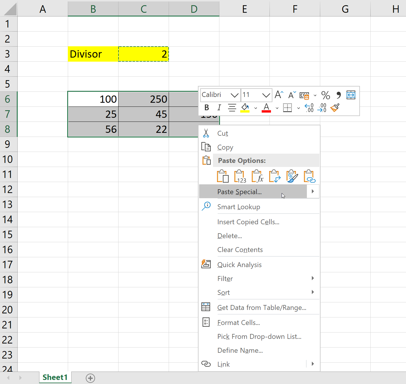
Assuming you don’t want to take the route of creating a formula that actually does the division, there are a couple of ways to go about this. First, if you really want to divide the values by 1,000, you could use the Paste Special feature of Excel:
- In a blank cell somewhere, enter the value 1000.
- Select the cell and press Ctrl+C. This copies the value to the Clipboard.
- Select the cells that you want to divide by 1,000.
- On the Home tab of the ribbon, click the down-arrow under the Paste tool. Excel displays a few options for your pasting pleasure.
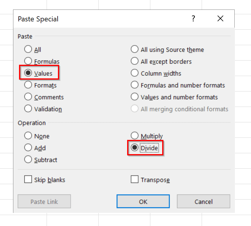
- Choose the Paste Special option. Excel displays the Paste Special dialog box. (See Figure 1.)
- In the Operation area of the dialog box, select the Divide radio button.
- Click OK.
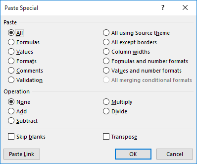
Figure 1. The Paste Special dialog box.
That’s it; all the cells you selected in step 3 are divided by 1000. You can also delete the value you placed in the cell in step 1.You should be aware that the Paste Special will work on all cells you selected, even if those cells are in hidden rows or columns.
If you don’t want to permanently modify your data, you could create a custom format that will display your data as if it were divided by 1,000. To do this, follow these steps:
- Select the range of cells you want to format.
- Right-click the range to display a Context menu, from which you should choose Format Cells. Excel displays the Format Cells dialog box.
- Make sure the Number tab is displayed.
- In the Category list, choose Custom. (See Figure 2.)
- In the Type box enter «##,##0.00,» (without the quote marks).
- Click OK.
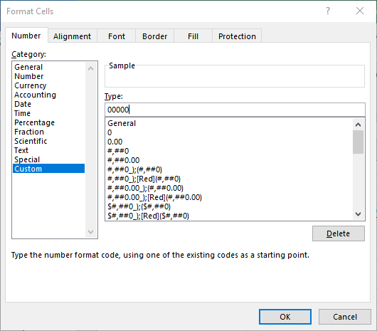
Figure 2. The Number tab of the Format Cells dialog box.
The cells now appear as if they’ve been divided by 1,000, even though the original values remain in the cells. If you prefer to «divide» by 1,000,000, then you can place two trailing commas in the custom format in step 5.
ExcelTips is your source for cost-effective Microsoft Excel training.
This tip (11229) applies to Microsoft Excel 2007, 2010, 2013, 2016, 2019, and Excel in Microsoft 365.
Author Bio
With more than 50 non-fiction books and numerous magazine articles to his credit, Allen Wyatt is an internationally recognized author. He is president of Sharon Parq Associates, a computer and publishing services company. Learn more about Allen…
MORE FROM ALLEN
Footnotes within Footnotes
Need to add footnotes to your footnotes? It’s actually allowed by some style guides, but Word doesn’t make it so easy.
Discover More
Offering Options in a Macro
It is often helpful to get user input within a macro. Here’s a quick way to present some options and get the user’s response.
Discover More
Getting Rid of Hidden Text in Many Files
Hidden text is a great boon if you want to make sure something doesn’t show up on the screen or on a printout. If you …
Discover More
Содержание
- Distribute the contents of a cell into adjacent columns
- Need more help?
- Multiply and divide numbers in Excel
- Multiply numbers
- Multiply numbers in a cell
- Multiply a column of numbers by a constant number
- Multiply numbers in different cells by using a formula
- Divide numbers
- Divide numbers in a cell
- Divide numbers by using cell references
- Multiply and divide numbers in Excel
- Multiply numbers
- Multiply numbers in a cell
- Multiply a column of numbers by a constant number
- Multiply numbers in different cells by using a formula
- Divide numbers
- Divide numbers in a cell
- Divide numbers by using cell references
- How to divide in Excel and handle #DIV/0! error
- Divide symbol in Excel
- How to divide numbers in Excel
- How to divide cell value in Excel
- Divide function in Excel (QUOTIENT)
- 3 things you should know about QUOTIENT function
- How to divide columns in Excel
- How to divide two columns in Excel by copying a formula
- How to divide one column by another with an array formula
- How to divide a column by a number in Excel
- Divide a column by number with a formula
- Divide a column by the same number with Paste Special
- How to divide by percentage in Excel
- Excel DIV/0 error
- Suppress #DIV/0 error with IFERROR
- Handle Excel DIV/0 error with IF formula
- How to divide with Ultimate Suite for Excel
Distribute the contents of a cell into adjacent columns
You can divide the contents of a cell and distribute the constituent parts into multiple adjacent cells. For example, if your worksheet contains a column Full Name, you can split that column into two columns—a First Name column and Last Name column.
For an alternative method of distributing text across columns, see the article, Split text among columns by using functions.
You can combine cells with the CONCAT function or the CONCATENATE function.
Follow these steps:
Note: A range containing a column that you want to split can include any number of rows, but it can include no more than one column. It’s important to keep enough blank columns to the right of the selected column, which will prevent data in any adjacent columns from being overwritten by the data that is to be distributed. If necessary, insert a number of empty columns that will be sufficient to contain each of the constituent parts of the distributed data.
Select the cell, range, or entire column that contains the text values that you want to split.
On the Data tab, in the Data Tools group, click Text to Columns.
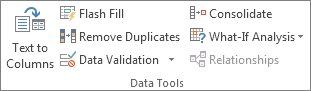
Follow the instructions in the Convert Text to Columns Wizard to specify how you want to divide the text into separate columns.
Note: For help with completing all the steps of the wizard, see the topic, Split text into different columns with the Convert Text to Columns Wizard, or click Help  in the Convert to Text Columns Wizard.
This feature isn’t available in Excel for the web.
If you have the Excel desktop application, you can use the Open in Excel button to open the workbook and distribute the contents of a cell into adjacent columns.
Need more help?
You can always ask an expert in the Excel Tech Community or get support in the Answers community.
Источник
Multiply and divide numbers in Excel
Multiplying and dividing in Excel is easy, but you need to create a simple formula to do it. Just remember that all formulas in Excel begin with an equal sign (=), and you can use the formula bar to create them.
Multiply numbers
Let’s say you want to figure out how much bottled water that you need for a customer conference (total attendees × 4 days × 3 bottles per day) or the reimbursement travel cost for a business trip (total miles × 0.46). There are several ways to multiply numbers.
Multiply numbers in a cell
To do this task, use the * (asterisk) arithmetic operator.
For example, if you type =5*10 in a cell, the cell displays the result, 50.
Multiply a column of numbers by a constant number
Suppose you want to multiply each cell in a column of seven numbers by a number that is contained in another cell. In this example, the number you want to multiply by is 3, contained in cell C2.
Type =A2*$B$2 in a new column in your spreadsheet (the above example uses column D). Be sure to include a $ symbol before B and before 2 in the formula, and press ENTER.
Note: Using $ symbols tells Excel that the reference to B2 is «absolute,» which means that when you copy the formula to another cell, the reference will always be to cell B2. If you didn’t use $ symbols in the formula and you dragged the formula down to cell B3, Excel would change the formula to =A3*C3, which wouldn’t work, because there is no value in B3.
Drag the formula down to the other cells in the column.
Note: In Excel 2016 for Windows, the cells are populated automatically.
Multiply numbers in different cells by using a formula
You can use the PRODUCT function to multiply numbers, cells, and ranges.
You can use any combination of up to 255 numbers or cell references in the PRODUCT function. For example, the formula =PRODUCT(A2,A4:A15,12,E3:E5,150,G4,H4:J6) multiplies two single cells (A2 and G4), two numbers (12 and 150), and three ranges (A4:A15, E3:E5, and H4:J6).
Divide numbers
Let’s say you want to find out how many person hours it took to finish a project (total project hours ÷ total people on project) or the actual miles per gallon rate for your recent cross-country trip (total miles ÷ total gallons). There are several ways to divide numbers.
Divide numbers in a cell
To do this task, use the / (forward slash) arithmetic operator.
For example, if you type =10/5 in a cell, the cell displays 2.
Important: Be sure to type an equal sign ( =) in the cell before you type the numbers and the / operator; otherwise, Excel will interpret what you type as a date. For example, if you type 7/30, Excel may display 30-Jul in the cell. Or, if you type 12/36, Excel will first convert that value to 12/1/1936 and display 1-Dec in the cell.
Note: There is no DIVIDE function in Excel.
Divide numbers by using cell references
Instead of typing numbers directly in a formula, you can use cell references, such as A2 and A3, to refer to the numbers that you want to divide and divide by.
The example may be easier to understand if you copy it to a blank worksheet.
How to copy an example
Create a blank workbook or worksheet.
Select the example in the Help topic.
Note: Do not select the row or column headers.

Selecting an example from Help
In the worksheet, select cell A1, and press CTRL+V.
To switch between viewing the results and viewing the formulas that return the results, press CTRL+` (grave accent), or on the Formulas tab, click the Show Formulas button.
Источник
Multiply and divide numbers in Excel
Multiplying and dividing in Excel is easy, but you need to create a simple formula to do it. Just remember that all formulas in Excel begin with an equal sign (=), and you can use the formula bar to create them.
Multiply numbers
Let’s say you want to figure out how much bottled water that you need for a customer conference (total attendees × 4 days × 3 bottles per day) or the reimbursement travel cost for a business trip (total miles × 0.46). There are several ways to multiply numbers.
Multiply numbers in a cell
To do this task, use the * (asterisk) arithmetic operator.
For example, if you type =5*10 in a cell, the cell displays the result, 50.
Multiply a column of numbers by a constant number
Suppose you want to multiply each cell in a column of seven numbers by a number that is contained in another cell. In this example, the number you want to multiply by is 3, contained in cell C2.
Type =A2*$B$2 in a new column in your spreadsheet (the above example uses column D). Be sure to include a $ symbol before B and before 2 in the formula, and press ENTER.
Note: Using $ symbols tells Excel that the reference to B2 is «absolute,» which means that when you copy the formula to another cell, the reference will always be to cell B2. If you didn’t use $ symbols in the formula and you dragged the formula down to cell B3, Excel would change the formula to =A3*C3, which wouldn’t work, because there is no value in B3.
Drag the formula down to the other cells in the column.
Note: In Excel 2016 for Windows, the cells are populated automatically.
Multiply numbers in different cells by using a formula
You can use the PRODUCT function to multiply numbers, cells, and ranges.
You can use any combination of up to 255 numbers or cell references in the PRODUCT function. For example, the formula =PRODUCT(A2,A4:A15,12,E3:E5,150,G4,H4:J6) multiplies two single cells (A2 and G4), two numbers (12 and 150), and three ranges (A4:A15, E3:E5, and H4:J6).
Divide numbers
Let’s say you want to find out how many person hours it took to finish a project (total project hours ÷ total people on project) or the actual miles per gallon rate for your recent cross-country trip (total miles ÷ total gallons). There are several ways to divide numbers.
Divide numbers in a cell
To do this task, use the / (forward slash) arithmetic operator.
For example, if you type =10/5 in a cell, the cell displays 2.
Important: Be sure to type an equal sign ( =) in the cell before you type the numbers and the / operator; otherwise, Excel will interpret what you type as a date. For example, if you type 7/30, Excel may display 30-Jul in the cell. Or, if you type 12/36, Excel will first convert that value to 12/1/1936 and display 1-Dec in the cell.
Note: There is no DIVIDE function in Excel.
Divide numbers by using cell references
Instead of typing numbers directly in a formula, you can use cell references, such as A2 and A3, to refer to the numbers that you want to divide and divide by.
The example may be easier to understand if you copy it to a blank worksheet.
How to copy an example
Create a blank workbook or worksheet.
Select the example in the Help topic.
Note: Do not select the row or column headers.
Selecting an example from Help
In the worksheet, select cell A1, and press CTRL+V.
To switch between viewing the results and viewing the formulas that return the results, press CTRL+` (grave accent), or on the Formulas tab, click the Show Formulas button.
Источник
How to divide in Excel and handle #DIV/0! error
 by Svetlana Cheusheva, updated on March 17, 2023
The tutorial shows how to use a division formula in Excel to divide numbers, cells or entire columns and how to handle Div/0 errors.
As with other basic math operations, Microsoft Excel provides several ways to divide numbers and cells. Which one to use depends on your personal preferences and a particular task you need to solve. In this tutorial, you will find some good examples of using a division formula in Excel that cover the most common scenarios.
Divide symbol in Excel
The common way to do division is by using the divide sign. In mathematics, the operation of division is represented by an obelus symbol (Г·). In Microsoft Excel, the divide symbol is a forward slash (/).
With this approach, you simply write an expression like =a/b with no spaces, where:
- a is the dividend — a number you want to divide, and
- b is the divisor — a number by which the dividend is to be divided.
How to divide numbers in Excel
To divide two numbers in Excel, you type the equals sign (=) in a cell, then type the number to be divided, followed by a forward slash, followed by the number to divide by, and press the Enter key to calculate the formula.
For example, to divide 10 by 5, you type the following expression in a cell: =10/5
The screenshot below shows a few more examples of a simple division formula in Excel: 
When a formula performs more than one arithmetic operation, it is important to remember about the order of calculations in Excel (PEMDAS): parentheses first, followed by exponentiation (raising to power), followed by multiplication or division whichever comes first, followed by addition or subtraction whichever comes first.
How to divide cell value in Excel
To divide cell values, you use the divide symbol exactly like shown in the above examples, but supply cell references instead of numbers.
- To divide a value in cell A2 by 5: =A2/5
- To divide cell A2 by cell B2: =A2/B2
- To divide multiple cells successively, type cell references separated by the division symbol. For example, to divide the number in A2 by the number in B2, and then divide the result by the number in C2, use this formula: =A2/B2/C2

Divide function in Excel (QUOTIENT)
I have to say plainly: there is no Divide function in Excel. Whenever you want to divide one number by another, use the division symbol as explained in the above examples.
However, if you want to return only the integer portion of a division and discard the remainder, then use the QUOTIENT function:
- Numerator (required) — the dividend, i.e. the number to be divided.
- Denominator (required) — the divisor, i.e. the number to divide by.
When two numbers divide evenly without remainder, the division symbol and a QUOTIENT formula return the same result. For example, both of the below formulars return 2.
When there is a remainder after division, the divide sign returns a decimal number and the QUOTIENT function returns only the integer part. For example:
=QUOTIENT(5,4) yields 1 
3 things you should know about QUOTIENT function
As simple as it seems, the Excel QUOTIENT function still has a few caveats you should be aware of:
- The numerator and denominator arguments should be supplied as numbers, references to cells containing numbers, or other functions that return numbers.
- If either argument is non-numeric, a QUOTIENT formula returns the #VALUE! error.
- If denominator is 0, QUOTIENT returns the divide by zero error (#DIV/0!).
How to divide columns in Excel
Dividing columns in Excel is also easy. It can done by copying a regular division formula down the column or by using an array formula. Why would one want to use an array formula for a trivial task like that? You will learn the reason in a moment 🙂
How to divide two columns in Excel by copying a formula
To divide columns in Excel, just do the following:
- Divide two cells in the topmost row, for example: =A2/B2
- Insert the formula in the first cell (say C2) and double-click the small green square in the lower-right corner of the cell to copy the formula down the column. Done!
Since we use relative cell references (without the $ sign), our division formula will change based on a relative position of a cell where it is copied: 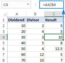
Tip. In a similar fashion, you can divide two rows in Excel. For example, to divide values in row 1 by values in row 2, you put =A1/A2 in cell A3, and then copy the formula rightwards to as many cells as necessary.
How to divide one column by another with an array formula
In situations when you want to prevent accidental deletion or alteration of a formula in individual cells, insert an array formula in an entire range.
For example, to divide the values in cells A2:A8 by the values in B2:B8 row-by-row, use this formula: =A2:A8/B2:B8
To insert the array formula correctly, perform these steps:
- Select the entire range where you want to enter the formula (C2:C8 in this example).
- Type the formula in the formula bar and press Ctrl + Shift + Enter to complete it. As soon as you do this, Excel will enclose the formula in , indicating it’s an array formula.
As the result, you will have the numbers in column A divided by the numbers in column B in one fell swoop. If someone tries to edit your formula in an individual cell, Excel will show a warning that part of an array cannot be changed.
To delete or modify the formula, you will need to select the whole range first, and then make the changes. To extend the formula to new rows, select the entire range including new rows, change the cell references in the formula bar to accommodate new cells, and then press Ctrl + Shift + Enter to update the formula. 
How to divide a column by a number in Excel
Depending on whether you want the output to be formulas or values, you can divide a column of numbers by a constant number by using a division formula or Paste Special feature.
Divide a column by number with a formula
As you already know, the fastest way to do division in Excel is by using the divide symbol. So, to divide each number in a given column by the same number, you put a usual division formula in the first cell, and then copy the formula down the column. That’s all there is to it!
For example, to divide values in column A by the number 5, insert the following formula in A2, and then copy it down to as many cells as you want: =A2/5 
As explained in the above example, the use of a relative cell reference (A2) ensures that the formula gets adjusted properly for each row. That is, the formula in B3 becomes =A3/5 , the formula in B4 becomes =A4/5 , and so on.
Instead of supplying the divisor directly in the formula, you can enter it in some cell, say D2, and divide by that cell. In this case, it’s important that you lock the cell reference with the dollar sign (like $D$2), making it an absolute reference because this reference should remain constant no matter where the formula is copied.
As shown in the screenshot below, the formula =A2/$D$2 returns exactly the same results as =A2/5 . 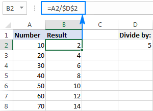
Divide a column by the same number with Paste Special
In case you want the results to be values, not formulas, you can do division in the usual way, and then replace formulas with values. Or, you can achieve the same result faster with the Paste Special > Divide option.
- If you don’t want to override the original numbers, copy them to the column where you want to have the results. In this example, we copy numbers from column A to column B.
- Put the divisor in some cell, say D2, like shown in the screenshot below.
- Select the divisor cell (D5), and press Ctrl + C to copy it to the clipboard.
- Select the cells you want to multiply (B2:B8).
- Press Ctrl + Alt + V , then I , which is the shortcut for Paste Special >Divide, and hit the Enter key.

Alternatively, right-click the selected numbers, select Paste Special… from the context menu, then select Divide under Operation, and click OK. 
Either way, each of the selected numbers in column A will be divided by the number in D5, and the results will be returned as values, not formulas: 
How to divide by percentage in Excel
Since percentages are parts of larger whole things, some people think that to calculate percentage of a given number you should divide that number by percent. But that is a common delusion! To find percentages, you should multiply, not divide. For example, to find 20% of 80, you multiply 80 by 20% and get 16 as the result: 80*20%=16 or 80*0.2=16.
In what situations do you divide a number by percentage? For instance, to find X if a certain percent of X is Y. To make things clearer, let’s solve this problem: 100 is 25% of what number?
To get the answer, convert the problem to this simple equation:
With Y equal to 100 and P to 25%, the formula takes the following shape: =100/25%
Since 25% is 25 parts of a hundred, you can safely replace the percentage with a decimal number: =100/0.25
As shown in the screenshot below, the result of both formulas is 400: 
For more examples of percentage formulas, please see How to calculate percentages in Excel.
Excel DIV/0 error
Division by zero is an operation for which there exists no answer, therefore it is disallowed. Whenever you try to divide a number by 0 or by an empty cell in Excel, you will get the divide by zero error (#DIV/0!). In some situations, that error indication might be useful, alerting you about possible faults in your data set.
In other scenarios, your formulas can just be waiting for input, so you may wish to replace Excel Div 0 error notations with empty cells or with your own message. That can be done by using either an IF formula or IFERROR function.
Suppress #DIV/0 error with IFERROR
The easiest way to handle the #DIV/0! error in Excel is to wrap your division formula in the IFERROR function like this:
The formula checks the result of the division, and if it evaluates to an error, returns an empty string («»), the result of the division otherwise.
Please have a look at the two worksheets below. Which one is more aesthetically pleasing? 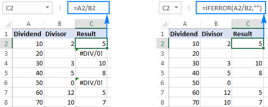
Note. Excel’s IFERROR function disguises not only #DIV/0! errors, but all other error types such as #N/A, #NAME?, #REF!, #VALUE!, etc. If you’d like to suppress specifically DIV/0 errors, then use an IF formula as shown in the next example.
Handle Excel DIV/0 error with IF formula
To mask only Div/0 errors in Excel, use an IF formula that checks if the divisor is equal (or not equal) to zero.
If the divisor is any number other than zero, the formulas divide cell A2 by B2. If B2 is 0 or blank, the formulas return nothing (empty string). 
Instead of an empty cell, you could also display a custom message like this:
=IF(B2<>0, A2/B2, «Error in calculation») 
How to divide with Ultimate Suite for Excel
If you are making your very first steps in Excel and do not feel comfortable with formulas yet, you can do division by using a mouse. All it takes is our Ultimate Suite installed in your Excel.
In one of the examples discussed earlier, we divided a column by a number with Excel’s Paste Special. That involved a lot of mouse movement and two shortcuts. Now, let me show you a shorter way to do the same.
- Copy the numbers you want to divide in the «Results» column to prevent the original numbers from being overridden.
- Select the copied values (C2:C5 in the screenshot below).
- Go to the Ablebits tools tab >Calculate group, and do the following:
- Select the divide sign (/) in the Operation box.
- Type the number to divide by in the Value box.
- Click the Calculate button.
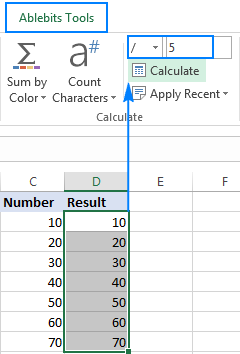
Done! The entire column is divided by the specified number in the blink of an eye: 
As with Excel Paste Special, the result of division is values, not formulas. So, you can safely move or copy the output to another location without worrying about updating formula references. You can even move or delete the original numbers, and your calculated numbers will be still safe and sound.
That is how you divide in Excel by using formulas or Calculate tools. If are curious to try this and many other useful features included with the Ultimate Suite for Excel, you are welcome to download 14-day trial version.
To have a closer look at the formulas discussed in this tutorial, feel free to download our sample workbook below. I thank you for reading and hope to see you on our blog next week!
Источник
There’s no DIVIDE function in Excel. Simply use the forward slash (/) to divide numbers in Excel.
1. The formula below divides numbers in a cell. Use the forward slash (/) as the division operator. Don’t forget, always start a formula with an equal sign (=).

2. The formula below divides the value in cell A1 by the value in cell B1.

3. Excel displays the #DIV/0! error when a formula tries to divide a number by 0 or an empty cell.

4. The formula below divides 43 by 8. Nothing special.

5. You can use the QUOTIENT function in Excel to return the integer portion of a division. This function discards the remainder of a division.

6. The MOD function in Excel returns the remainder of a division.

Take a look at the screenshot below. To divide the numbers in one column by the numbers in another column, execute the following steps.
7a. First, divide the value in cell A1 by the value in cell B1.

7b. Next, select cell C1, click on the lower right corner of cell C1 and drag it down to cell C6.

Take a look at the screenshot below. To divide a column of numbers by a constant number, execute the following steps.
8a. First, divide the value in cell A1 by the value in cell A8. Fix the reference to cell A8 by placing a $ symbol in front of the column letter and row number ($A$8).

8b. Next, select cell B1, click on the lower right corner of cell B1 and drag it down to cell B6.

Explanation: when we drag the formula down, the absolute reference ($A$8) stays the same, while the relative reference (A1) changes to A2, A3, A4, etc.
If you’re not a formula hero, use Paste Special to divide in Excel without using formulas!
9. For example, select cell C1.

10. Right click, and then click Copy (or press CTRL + c).
11. Select the range A1:A6.
12. Right click, and then click Paste Special.
13. Click Divide.

14. Click OK.

Note: to divide numbers in one column by numbers in another column, at step 9, simply select a range instead of a cell.
You can use the «divisible by» operation in Excel documents to solve problems such as uniformly allocating resources to a certain number of people. Even though this operation is not part of the list of standard operations, you can define it using two other functions, if and mod. These use the idea that if the remainder for the division of two numbers is 0, then the first number is divisible by the second.
-
You can combine the two expressions into a single one, so you don’t have to use two cells to express the divisibility property. Type «=IF(MOD(cell1,cell2)=0,’Divisible’,’Not divisible’)» (without double quotes) into an empty cell, where cell1 and cell2 are the names of the two cells holding the numbers.
Launch your Microsoft Excel document. Locate the two numbers you want to check the divisibility property for and note the name of their corresponding cells. The name of a cell is composed of a letter and a number. For example, the first cell of the first row in your document is labeled «A1.»
Click on an empty cell in your document and type «=MOD(cell1,cell2)» (without the quotes) inside it, where cell1 and cell2 are the names of the cells holding the two numbers. Press «Enter» to compute the remainder for the division of the two numbers.
Click on another empty cell and type «=IF(cell=0,’Divisible’,’Not divisible’)» (without double quotes) inside it, where cell is the name of the cell holding the remainder of the division. Press «Enter.» If the first number is divisible by the second one, Excel displays «Divisible» in this cell. if it isn’t, the software shows the message «Not divisible.»
Tips
How to Divide in Excel: Division Formula and Examples (2023)
If Microsoft Excel can do complex calculations and analysis, then performing simple calculations like division is as easy as pie 😎
Though you can let Excel do the math for you, you must understand how to divide numbers in Excel so you can work more accurately and efficiently 👨🏫
In this article, you’ll learn different methods of how to divide in Excel and some useful tips about dividing in Excel along the way.
Let’s dive in! 😀
Division in Excel
There is no DIVIDE function in Excel.
So when you want to divide numbers in Excel, use the forward slash (/) arithmetic operator.
To divide two numbers in Excel, you need to follow the division formula =a/b where:
- a – the dividend, the number you want to divide
- b – the divisor, the number you want the dividend to be divided by
It’s important to note that you need to first type the equal sign (=) in the cell before you type the numbers and the forward-slash (/) arithmetic operator.
If you don’t, Excel will interpret what you type as a date.
Say you want to divide 10 by 2, to do that…
- Double-click an empty cell.
- Type the formula =10/2 in the cell or in the formula bar.

- Press Enter.

Excel displays 5 as the quotient.
Here are other examples of how to do simple division formula in Excel 😊

What’s amazing in Excel is that you can use cell references in the division formula instead of typing numbers directly.
Learn more about this in the next section 👇
How to divide cells in Excel (using references)
As you know, you can input values in the cells of your worksheet.
So when you divide in Excel, you can just click the cell that contains the numbers you want to divide and divide by 😀
For example, if you want to divide 10 by 2, you can click the cell references that contain these numbers.
You can find the cell reference in the name box found to the left of the formula bar.

Let’s try it 💪
Let’s divide 10 by 2 again but this time using cell references.
- Double-click an empty cell and type the equal sign (=) to start the formula.

- Instead of typing 10, click the cell reference which has a cell value of 10.
In our example, it’s cell B3.
Then type the forward slash (/) arithmetic operator.

- Next, instead of typing 2, click the cell reference which has a cell value of 2.
In our example, it’s cell B5.

- Press Enter.

Excel shows you the quotient of the formula which is 5 👍
Below are other examples of how to divide in Excel using cell references.

If you divide a number by 0 or select an empty cell reference, Excel displays the #DIV/0! error.
So, make sure you click the cell references correctly when you divide numbers.
With the use of cell references, you’re not typing numbers directly in the cell.
This is super helpful especially when you have data already entered into the cells of the worksheet.
Easy, right? 😊
Order of operations
When performing arithmetic operations in Excel, it’s important for you to recall and understand the order of operations.
Without understanding the order of operations, the results may not what you expect 🤔
The order in which Excel performs operations in formulas is PEMDAS.
PEMDAS stands for Parentheses, Exponents, Multiplication or Division (whichever comes first), Addition or Subtraction (whichever comes first).
For example, in the Excel formula =10/2+3, you need to perform two arithmetic operations: division and addition 👨🏫
Following the PEMDAS, you need to perform first the division and then addition.
So Excel divides 10 by 2 first and then adds 3.
Excel displays 8 as the result.
The table below shows more examples of how the order of operations can impact division formulas.

PROTIP:
You can also use the QUOTIENT function in Excel. The quotient returns only the integer portion of a division and discards the remainder.
The QUOTIENT function has the syntax: =QUOTIENT(numerator,denominator)
Where:
- Numerator (required) – the dividend, the number you want to divide
- Denominator (required) – the divisor, the number you want the dividend to be divided by
You can see the difference between the simple formula for division and the QUOTIENT function in the table below 😊

As you can see, the QUOTIENT function only returns the integer portion of a division and discards the remainder.
So, Excel displays 3.
That’s it – Now what?
You got it! 👏
Though dividing is such a basic operation, it’s important that you understand how division works in Excel.
Now, you can confidently perform basic Excel formulas and functions in Excel 😀
Excel formulas and functions are what make Microsoft Excel a powerful spreadsheet program. It’s also the most used, that’s why Excel skills are in high demand 🚀
Kickstart your Excel journey and build your Excel skills to stand out.
Join my FREE Excel Beginner Training where you’ll learn the basics of Excel in the way you want–easy, on-point, and free 😊
Other resources
When using cell references in your Excel formulas, it’s important to know the difference between absolute, mixed, and relative cell references.
Read our Cell References article to learn more.
You might come across the #DIV/0 Error when you divide numbers in Excel. This article will guide you how to fix this Excel error.
I hope you find these helpful 🤗
Kasper Langmann2023-03-27T11:22:19+00:00
Page load link
This guide will show you how you can divide a range of cells by a number in Excel.
This operation is useful if you need to scale down an entire range of values. We will show you how to do this using the Paste Special tool and your typical Excel formulas.
Let’s take a look at a quick example where we might need to divide a range of cells by a specific number.
We have a list of values that range from 1 to 200. These values correspond to examination results for a test given to college students. We want to divide all values by 200 to get the percentage.
How do we do this easily in Microsoft Excel?
There are two quick methods to get the result we need. First, we can use the Paste Special option to apply a Divide operation on the entire range. Second, we can use a formula to create a second range of quotients from the input range.
To better understand how useful this operation is, let’s look at some examples of this formula working in Excel.
A Real Example of Dividing a Range of Cells by a Number in Excel
This section will show a real example of dividing a range of cells in an Excel spreadsheet.
In the example below, we have a range of values in B6:D8. Using simple Excel formulas, we can create another range of values, but all the numbers have been halved this time.
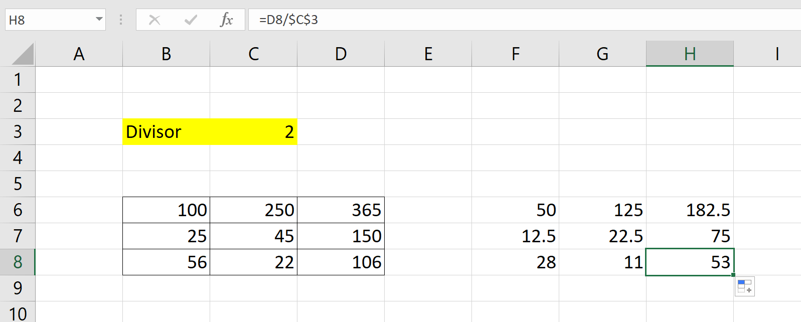
To get the values in Column C, we just need to use the following formula:
=B6/$C$3
The formula above will give us the upper-leftmost value in the range. We created an absolute reference to cell C3 so that we can fill the rest of the range without changing the divisor.
In the example below, we’ve used the same technique to divide the range B12:C17 by 200. The result is equivalent to the percentage of the original value with respect to the maximum score of 200.

We can change the formatting of the new range to create a more readable percentage.

You can make your own copy of the spreadsheet above using the link attached below.
All the sheets above will also work with the Paste Special tool. If you’re ready to learn about how you can achieve this in Excel, head over to the next section!
This section will explain each step needed to divide an entire range of cells by a single number. You’ll learn how we can use the Paste Special tool and basic Excel formulas to achieve this result.
First, we’ll explain how you can use the Paste Special technique.
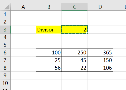
- Select the cell that holds the divisor. This is the number we want to divide the range by. In this example, we’ll be dividing the range B6:D8 by two.

- After selecting the cell, press Ctrl + C to copy the cell’s contents.

- Next, select the entire range we’ll be dividing by two. In the example below, we’ve selected the cell range B6:D8.

- Right-click anywhere within the range to bring up the menu. Select the Paste Special… option. We can also press Ctrl + Alt + V to bring up the Paste Special dialog menu.

- In the Past Special pop-up menu, select the following settings below. We will select Values to indicate that we want the numerical value we copied earlier for the Paste option. We select Divide for the Operation option. This allows values within the range to be divided by the number we’ll be “pasting” in this action.

Click OK to perform the operation. - Your original range should now be divided by the specified number. In the example below, you can see that the range has been halved.


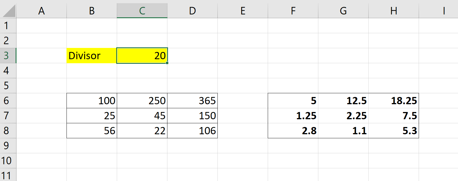
Alternatively, we can use Excel formulas to create a new range. This has the benefit of keeping the original values. We can also dynamically change the divisor later on if needed.
- We simply have to divide each cell by the given divisor using cell references for this to work. To easily fill out the range later on, we can make an absolute reference to our divisor so that it remains the same value.

- In the example below, we expanded the formula outward to achieve the same result.

- Changing the value of our divisor will dynamically change the values in our new range as well.


Frequently Asked Questions (FAQ)
- What is the difference between Paste and Paste Special?
The Paste Special feature is more powerful than your typical Paste operation. This feature gives you control over whether to copy the value, formatting or other source cell properties when pasting to another cell. The Paste Special feature also lets you perform operations on target cells, which is why it’s useful for dividing a range of cells.
That’s all you need to remember to start using the Paste Special tool in Microsoft Excel to divide an entire range. This step-by-step guide shows how easy it is to scale multiple values down by a certain number. We can use this tip to find percentages easily.
Using functions to divide a range of cells by a single number is just one example of a time-saving trick that you can apply in Excel. With so many other Excel functions out there, you can surely find a few that makes your spreadsheets more powerful.
Are you interested in learning more about what Excel can do? Make sure to subscribe to our newsletter to be the first to know about the latest guides and tutorials from us.

Get emails from us about Microsoft Excel.
Our goal this year is to create lots of rich, bite-sized tutorials for Microsoft Excel users like you. If you liked this one, you’d love what we are working on! Readers receive ✨ early access ✨ to new content.

Hi! I’m a Software Developer with a passion for data analytics. Google Sheets has helped me empower my teams to make data-driven decisions. There’s always something new to learn, so let’s explore how you can make life so much easier with spreadsheets!
In the past here at Chandoo.org and at many many other sites, people have asked the question “How can I display a number Multiplied or Divided by 10, 100, 1000, 1000000 etc, but still have the cell maintain the original number for use in subsequent calculations“.
Typically the answer has been limited to “It can’t be done” or “It can only be done in multiples of 1000”.
Well thanks to a tip I picked up from Kyle who responded to a post here at Chandoo.org they are all wrong.
It is possible to Multiply or Divide any cell contents by any power of 10 using Custom Number Formats !
That is:

How does this work:
When using custom number format we have two possibilities to modify the display number
- Use a Comma to divide by 1000; or
- Use a % to Multiply by 100
So using a combination of these any power of 10 can be obtained.

So using the correct combination of , and % can result in any power of 10 multiplier we require.
The problem is that using a % adds a % to the number!
The trick which Kyle added is that adding a Ctrl J to the Custom Number format allows us to hide the % signs on a second row of text, then by adjusting the cell to have word wrap and adjusting the row height the second row is not visible.
The Ctrl J must be added after the ,’s and before the %’s
So using the examples above the table is:

The Ctrl J adds a Carriage Return, chr(10), to the Format String.
Finally after applying the Custom Number Format the Cell must be edited to enable Word Wrap.
Select the Cells with the custom Formats, Ctrl 1, Alignment

You can see the hidden % symbols if you increase the Row Height.

Combination with Regular Custom Formats
These Custom Number Formats can of course still be combined with regular Custom Number Formats, just make sure that the Ctrl J is inserted before the % signs:

No Loss of the Cells Value
It is also worth noting that the original number is still maintained internally in the cell and that cells dependent on the cells don’t have to adjust for the display value.

Multi Line Formats
By extension we can now use this technique to add multiple Lines of Text to a Custom Number Format

Downloads
You can download a file containing all the above example here: Download Here
Other Links to Custom Number Formats
Here:
http://chandoo.org/wp/2008/02/25/custom-cell-formatting-in-excel-few-tips-tricks/
http://chandoo.org/wp/2011/11/02/a-technique-to-quickly-develop-custom-number-formats/
http://chandoo.org/wp/2011/08/19/selective-chart-axis-formating/
http://chandoo.org/wp/2011/08/22/custom-chart-axis-formating-part-2/
http://chandoo.org/wp/tag/custom-cell-formatting/
Elsewhere
http://www.ozgrid.com/Excel/CustomFormats.htm
http://peltiertech.com/Excel/NumberFormats.html
Thanx
Just a quick final Thank You to Kyle for highlighting this Custom Number Format feature/trick last week
I look forward to your comments below:
Share this tip with your colleagues

Get FREE Excel + Power BI Tips
Simple, fun and useful emails, once per week.
Learn & be awesome.
-
60 Comments -
Ask a question or say something… -
Tagged under
Custom Number Format
-
Category:
Excel Howtos, Huis, Posts by Hui

Welcome to Chandoo.org
Thank you so much for visiting. My aim is to make you awesome in Excel & Power BI. I do this by sharing videos, tips, examples and downloads on this website. There are more than 1,000 pages with all things Excel, Power BI, Dashboards & VBA here. Go ahead and spend few minutes to be AWESOME.
Read my story • FREE Excel tips book


Excel School made me great at work.
5/5

From simple to complex, there is a formula for every occasion. Check out the list now.

Calendars, invoices, trackers and much more. All free, fun and fantastic.

Power Query, Data model, DAX, Filters, Slicers, Conditional formats and beautiful charts. It’s all here.

Still on fence about Power BI? In this getting started guide, learn what is Power BI, how to get it and how to create your first report from scratch.

- Excel for beginners
- Advanced Excel Skills
- Excel Dashboards
- Complete guide to Pivot Tables
- Top 10 Excel Formulas
- Excel Shortcuts
- #Awesome Budget vs. Actual Chart
- 40+ VBA Examples
Related Tips
60 Responses to “Custom Number Formats (Multiply & Divide by any Power of 10)”
-
 Luke M says:
 Okay, that is pretty awesome. Thanks for the tip Kyle & Hui!
-
Steve Slaman says:
This gets me closer to a solution for reporting financial in (000’s) but I am still left with the rounding problem when adding these numbers. As an example 1,234,567 using 0,###, I get 1,235 which is great but when I sum 1,234,567 and 1,234,567 in this format 1,235 + 1,235 I get 2,469 instead of 2,470. 2,469 is technically correct, but for those who cannot see the full number the sum appears incorrect. Is there a fix for this?
-
Cameron says:
Steve, I often have to display numbers in a similar fashion. I have to ask though, is it wise or even necessary to force the display to ‘2,470’? As long as it is understood that some rounding is going on, it should be acceptable that the numbers won’t add up on screen. In fact displaying these incorrectly (outside of the realm of rounding) seems misleading?
Often, I will include somewhere on the page, prominently enough to be seen but not obtrusive, «In Thou.» or «In Mils.»
Alternatively you could make the custom format «#,K» which automatically suggests rounding.
-
Steve Slaman says:
I hear you, but that all numbers tie is absolutely expected at my company. As a former CFO explained to me years ago, if the numbers don’t add up it brings into question the validity of the report (as he chucked my report into the trash). Experience has taught me that he was absolutely right. This can take Sr. Management and Board of Directors off the focus of what the report and presentation is about. So the hours it takes me to tick and tie the reports is well spent (and cheap) compared to the time spent and repercussions up the ladder. I wish we could show the complete numbers in these presentation reports (30 slides per quarter) but it is just too busy on the screen.
I do put (000’s) at the top left of each report (we report in thousands).
Thanks for your response!
-
Kyle McGhee says:
Well, there really is no way to solve it other than rounding to the nearest X. (since that is what Excel is doing with the format, rounding to the nearest 1000)
Here is a formula, for a total, that rounds each number in A1 to A100 to the nearest 1000 and then sums it up.
=SUMPRODUCT(ROUND(A1:A100,-3))
It has the same effect has rounding each individually but it leaves the individual items alone so you can keep accurate percentages.-
Steve Slaman says:
You are right, the fact is we are taking away three places in each number by rounding to thousands and holes are naturally created that must be filled or explained. But it is still great to have the discussion. I learn about how others think and put another tool or two in my Excel toolbox.
I greatly appreciate this!!
-
-
-
-
Kyle McGhee says:
Steve,
I have to agree with Cameron. I made a similar post yesterday morning that was lost with the server migration. There is a certain level of displayed inaccuracy that is expected when reporting in 000s or 00s. It is best to leave everything as is, which will provide the most accurate results. As Cameron suggested, stating it is in 000s would be the best approach, and if desired, stating that there may be rounding differences as well. I work in finance/accounting as well and I never round except for check totals (due to the floating point issues).
Kyle
-
Steve Slaman says:
I really appreciate your response. You are both correct with expected inaccuracies. In my situation, the inaccuracies are best done in plugs. If I have to round one of the larger numbers (say advertising) up or down 1 (1,000) to get the number to balance it is much cleaner and reduces questions. Of course it also takes more time and makes the process manual.
-
-
-
Kyle McGhee says:
Try this:
=(ROUND(A1,-3)+ROUND(A2,-3))
-
Steve Slaman says:
Thanks for the post. I currently use the round commands (round, roundup and rounddown) but was hoping to get away from that. In a simple or single sum the round command works well but when I start using those rounded sums to get to a bottom line (Profit/Loss) or on a balance sheet, they can veer out of balance from actual final numbers more often than I like to see. It especially gets ugly in % change. I spend a lot of time verifying that everything tics and ties. I’m still going to try this format on my next financial presentation with the rounds to see how well it works.
Thanks again!!
-
-
Another handy technique is to use the text function. For example, to display a date in a format that you want, you can do something like:
=text( A1, «yyyy-MM-dd» )
Lots of potential variations there, but it lets you format A1 however you want it, without altering it.
side note, in some languages, I’ve seen other choices such as «jjjj-MM-dd» so if you care about internationalization, try to make your formatting easy to change by making the format text refer to a single cell.
-
Jonathan Cohen says:
Try setting precision as diplayed in the advanced options.
-
Steve Slaman says:
Thanks. This is a cool new feature to me, unfortunately in this instance the original number is lost to the rounded number (1,234,567 becomes 1,235,000). Great tip for future reference, I’m already thinking of ways I can use it.
Thanks again!!
-
-
Arti K says:
Excellent tip! Thank you.
-
nice.. post
Regards,
Saran
lostinexcel.blogspot.com -
Steve, this is an excellent tip. But with the % sign used to Multiply, the symbol still shows up in the cells, even with usage. Am I missing anything else?
-
@Dhakkanz
Did you put a Ctrl J in front of the % sign ?-
Que says:
The Ctrl J trick works but not very well if the space is limited. For example, I want to show 9E-12 as 9 (units is in picoseconds). If I limit the cell width to less than 10 characters then this trick does not work.
Any other suggestions if the space is limited?
-
-
-
bill says:
this is very clever. i like the concept. there is something about the concept that makes me uneasy… i think it is reading this article after having finished the great series of articles on auditing and spreadsheet risk….
-
bill says:
i recently stumbled on a software company that was addressing the rounding and or formatting creating incorrect sums (visible) issue. their solution seemed hard to implement and has costs but does work quite well. i think a well written vba program would be more flexible (for solving rounding/formatting issues). here is their link:
http://www.think-cell.com/products/round/overview.shtml -
Sugandh says:
I was so happy to see such a custom format. I had not imagined that there would be such a simple solution to the problem. Thanks a lot.
This post will be very useful to Engineers like me who have to do a lot of electrical design calculations in excel. Very often we have to deal with *1000 or /1000 value of current or voltage For ex. millivolts mV, milliampere mA, milliwatt mW.
With this formatting trick, I can now remove all the *1000 or /1000 I had to add in my formulas to take care of the multiplier factor.
🙂
However,
I have one new problem using this custom format. My Excel uses German standard way of representing numbers i.e. a «comma» to denote decimal point and a «dot or punkt» to denote thousands (‘1000s) placeholder. Alos, eventually the sheets I make will be read on German Excel only.Can someone post a German equivalent to the same formatting?
Thanks again.
-
Nima says:
Thanks very much.
The trick was very usefull.
Problems will be very simple when they are solved!
Thanks again. -
[…] Microsoft – Custom Number Formatting > Chandoo – Factor 10 number scaling > ASAP Utilities – Create a bulleted list > Daily Dose of Excel – Star Rating […]
-
[…] Microsoft – Custom Number Formatting > Chandoo – Factor 10 number scaling > ASAP Utilities – Create a bulleted list > Daily Dose of Excel – Star Rating […]
-
Ivan says:
Hi Thank you for the tutorial. It is very useful and clear.
And I have a question related to this format.
Is it possible to multiply by a different number instead of 10?
I don’t want to create a new column to do the multiplication.Let’s say it will automatically multiply 2 when I enter 19 and will show 38 in the cell.
Thanks for reading and hope you could help me.
-
Matt says:
OK so I’m trying to use this to format a cell so that this:
0.09
0.07
-0.14Will display as:
9.0%
7.0
(14.0)Looking to have the decimal points align but not show the % symbol after the first row. The problem with the above technique is that formating the wrap text will eliminate any placeholders you put in place to help with the alignment formating. Is there any workaround to this?
-
@Matt
Are the 3 values in the same cell?
If so I doubt you can do what you want
-
-
Matt says:
Different cells, just gave 3 as an example. Effectively the cell would multiply by 100 but still give the spacing as if a % were there, ie putting a _% effect at the end of the cell
-
@Matt
If I use the format
#,#Ctrl J%
I get:
9
7
-14You have to enable Word Wrap in those cells
and then adjust the width accordingly
-
-
[…] Hi, You can do this with custom number formatting. There are limits to what you can do with it, but for your specific example, a format like this might work: 0000″ / (4837)» To learn more about custom number formatting see: Create or delete a custom number format — Excel — Office.com Excel Custom Formats: Numbers/Text Formats in Excel Spreadsheets Custom Number Formats (Multiply & Divide by any Power of 10) | Chandoo.org — Learn Microsoft Exc… […]
-
Suzie says:
okay idk what i did wrong, maybe my excel is being stupid but its not working 🙁
i originally have 52.6625 (it’s in thousands) so it’s really 52,662.50.
if I put in the *1000 formatting above i get this result:
52,662.5%%%
if I try it without the carrots i get:
52,662.5CtrlJ%%%
Also if I go back into the custom formatting, it changed it to:
#,###.#%%%I dont know why it put a «/» in between the Ctrl either. Any suggestions as to what I’m doing wrong??
Thanks!
-
Suzie says:
nvm! im dumb and realized you don’t type the control j but actually hit control+j
-
mathew varghese says:
Dear Hui,
I have been reading your posts with awe. Thanks to Chandoos’s work. I need your help. How do I custom format a number to display in lakhs as used in India…..123456789.00 as 12,34,56,789.00 (twelve crores thirty four lakhs fifty six thousand seven hundred eighty nine…..I understand excel will show numbers in thousands only….Thanks
-
Caron says:
Thanks for this tip. I have two questions:
1. I need to divide numbers by 1000 but leave no decimals.
At the moment the format I’m using from your site is # ##0.###.
However, this is leaving me with a result with a . on the end.
i.e 1000 becomes 1. instead of just 1 with no point on the end.2. My spreadsheets has a number of pivot tables representing a sheet that automatically updates from the accounting database.
So lots of ways of analyzing sales.
Is there a way I can set the format once for a value instead of having to format on every sheet?All help much appreciated
-
-
Caron says:
Thanks! will give it a try.
Caron
-
-
-
Brian says:
Unfortunately it seems this work-around has now been semi-disabled in Excel 2010.
When you first enter the number format, the application accepts it and everything works fine. But if you save the file and re-open it: excel has modified the number format, and it breaks the functionality.
Specifically: all the formats that make use of a comma AND percentage sign in the same (sub)-format, excel now DELETES all trailing commas in the saved custom-number-format string. Hence when you reopen the file all formats like «mA» or «mV» are now displayed 1000x their actual value.
Example:
Try to apply: 0.0,»mV»%%%
Excel will strip the comma and save it as: 0.0″mV»%%%
(which obviously won’t produce the desired effect)Funny enough, excel WILL apply the correct number format TEMPORARILY to the open document: but if you re-open the file, POOF! all number formats wrecked.
(Perhaps older versions always saved the number format wrongly too, and they have changed the way number formats are refreshed upon opening the file. Or they could have purposely disabled this — who knows)
So sad. This was an almost perfect work-around.
I would be interested which versions of Excel this still works in. -
James says:
Hi,
Is there a way to automatically include the 2 digit year into a custom format for invoice numbering …?
Is there a trick to combine functions (such as today() or year()..) in a given custom format ?
Thanks -
Johnd239 says:
You could certainly see your skills within the work you write. The world hopes for more passionate writers like you who arent afraid to say how they believe. Always follow your heart. cgaedfkafgde
-
Johnb136 says:
I think you have observed some very interesting details , appreciate it for the post. kabddabcdfag
-
Roshan says:
Hi,
Is there a way to add 100 to only the number format? I have a graph which shows the diff from 100, e.g. 89 is -ve 11 from 100 and 139 is +ve 39. I want my graph to calculate based on -11 & 39 but shows 89 & 139. I can do this for the positive number using the format #,##100 but it shows -111 instead of 89 for the negative.
Not sure if I was very clear in what I was looking for, but any help is appreciated.
Thanks,
Roshan-
Roshan says:
just to update that, I need only the data labels for the graph to show 89 & 139
-
-
Deepak vats (Chandigarh) says:
dear Sir
Thanks
-
Deepak vats (Chandigarh) says:
Dear Sir
I read your article. I want to display absolute figures in lacs —
/1000000Put 0.######,,,%% in Custom Number formatting
want Rs. 1662052 as 16.62
but getting as 1.6222052%%
Trying Ctrl+J as madam kyle suggested but %% are reflecting on excel screen and not getting hided so cannot send report to Top Management. Kindly assist. I think I am making a mistake in Ctrl+J step.Thanks a lot in advance.
warm regards,
Deepak Vats -
@Hui
Sir great work, you helped me alot.
Thanks for sharing wonderful tricks.@Deepak
First make your cell vertical alignment to top + wrap text
then use this in custom format:
#,##0.00,,, %%
Press Ctrl+J before %It will looks like:
#,##0.00,,,
%%and you are done.
Regards, -
VSM says:
Hi Guys,
I have created custom format ##,##0.0,,, CTRL + J %% to display
10000 as 0.1
100000 as 1.0
1000000 as 10.0
10000000 as 100.0
100000000 as 1,000.0
so forth.The problem i am facing is that once i applied this format , save and close the workbook. the next time i open it the format get change like for 100000 it shows me 1.0 before closing the workbook ans 10.0 when i open it again.
please adviceVSM
-
VSM says:
Any help guys!
VSM
-
VSM says:
How can i attached the images here
-
-
-
Rachel says:
I am trying to utilize this technique in order to calculate basis points. Basis points multiple % by 10,000 in order to find their value. For example, 1% would be 100 bps. I have a % field that calculates the bps % and then used the formatting of #,#.#%% to try and arrive at the formatting for bps. However, since the field is linked to a percentage, it is formatting as 100%%. I need the percentages to be removed and a «bps» to be replaced.
-
@Rachel
I don’t believe that what you want can be done in 1 cell
You may have to use a helper column to assist you-
Rachel says:
Hi Hui — I don’t have the option to create another field as I am already using a calculated field to arrive at %. To find the bps, I calculated MU% in a calculated field. I then pulled in the MU% field again and found the «Difference from» to find the % change. I then formatted the % change to x10,000 but it’s not showing up correctly.
-
-
-
Martin Mat?jka says:
Great trick, thanks a lot!
I have used it to show pp instead of %,
my custom format looks like this:0″pp?»%
-
I have noticed that this method works well with .xls files in compatibilty mode. However, I have had trouble with it using .xlsx files. Specifically, I can get the method to work in the newer formats on initial capture, but when I save, close, and reopen the workbook, it does not work after the reopen – the control-j seems to vanish.
Has anyone else seen this behavior?
-
raj says:
Hi Mark,
We too are facing similar issue. We are using office 365 version of excel. Did you find any workaround for this issue.
-
-
Robin says:
With all the format codes I was finding I couldn’t shrink the excel cell width without the numbers turning to #####.
Apply shrink to fit, then word wrap and all was good. -
raj says:
Firstly i would like to thank you for the solution you provided.
As Mark and Brian has mentioned, we too are facing the similar issue. The custom formatting disappears after saving and reopening the excel file. We are using Office365 version.
The custom format that we are using is :
0.#####,,,%%
0.#####0,,,%%
Any help would be highly appreciated. -
Rohit Maloo says:
Hi People,
The article is amazing!!
I am looking to divide numbers by 100.
I am using conditional formatting, wherein when a user selects «Hundreds» from the dropdown menu, entire numbers in all worksheets get divided by 100 and if one chooses, «Normal», normal numbers are displayed.Now it is working properly, however, when I close and reopen the excel sheet, the entire formatting changes.
Any workaround?
I need to display normal as well as divide by 100 numbers.I am using excel 365, any new function in it?
Thanks,
Rohit -
Robert Honeyman’ says:
I used this a couple of years ago to discover use of the comma. I had a vague recollection that you described how to go in the opposite direction.
When I couldn’t figure out how to hide the percent signs even using , I downloaded your example file. That file is an xls file and it opened in compatability mode. I wonder if you have a solution for Office 365, or it I would have to save my file in an earlier version of Excel (I won’t do it, BTW). Thanks.
Best regards,