Split text into different columns with functions
Excel for Microsoft 365 Excel for Microsoft 365 for Mac Excel for the web Excel 2021 Excel 2021 for Mac Excel 2019 Excel 2019 for Mac Excel 2016 Excel 2016 for Mac Excel 2013 Excel Web App Excel 2010 Excel 2007 Excel for Mac 2011 More…Less
You can use the LEFT, MID, RIGHT, SEARCH, and LEN text functions to manipulate strings of text in your data. For example, you can distribute the first, middle, and last names from a single cell into three separate columns.
The key to distributing name components with text functions is the position of each character within a text string. The positions of the spaces within the text string are also important because they indicate the beginning or end of name components in a string.
For example, in a cell that contains only a first and last name, the last name begins after the first instance of a space. Some names in your list may contain a middle name, in which case, the last name begins after the second instance of a space.
This article shows you how to extract various components from a variety of name formats using these handy functions. You can also split text into different columns with the Convert Text to Columns Wizard
|
Example name |
Description |
First name |
Middle name |
Last name |
Suffix |
|
|
1 |
Jeff Smith |
No middle name |
Jeff |
Smith |
||
|
2 |
Eric S. Kurjan |
One middle initial |
Eric |
S. |
Kurjan |
|
|
3 |
Janaina B. G. Bueno |
Two middle initials |
Janaina |
B. G. |
Bueno |
|
|
4 |
Kahn, Wendy Beth |
Last name first, with comma |
Wendy |
Beth |
Kahn |
|
|
5 |
Mary Kay D. Andersen |
Two-part first name |
Mary Kay |
D. |
Andersen |
|
|
6 |
Paula Barreto de Mattos |
Three-part last name |
Paula |
Barreto de Mattos |
||
|
7 |
James van Eaton |
Two-part last name |
James |
van Eaton |
||
|
8 |
Bacon Jr., Dan K. |
Last name and suffix first, with comma |
Dan |
K. |
Bacon |
Jr. |
|
9 |
Gary Altman III |
With suffix |
Gary |
Altman |
III |
|
|
10 |
Mr. Ryan Ihrig |
With prefix |
Ryan |
Ihrig |
||
|
11 |
Julie Taft-Rider |
Hyphenated last name |
Julie |
Taft-Rider |
Note: In the graphics in the following examples, the highlight in the full name shows the character that the matching SEARCH formula is looking for.
This example separates two components: first name and last name. A single space separates the two names.
Copy the cells in the table and paste into an Excel worksheet at cell A1. The formula you see on the left will be displayed for reference, while Excel will automatically convert the formula on the right into the appropriate result.
Hint Before you paste the data into the worksheet, set the column widths of columns A and B to 250.
|
Example name |
Description |
|
Jeff Smith |
No middle name |
|
Formula |
Result (first name) |
|
‘=LEFT(A2, SEARCH(» «,A2,1)) |
=LEFT(A2, SEARCH(» «,A2,1)) |
|
Formula |
Result (last name) |
|
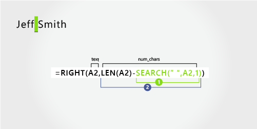
‘=RIGHT(A2,LEN(A2)-SEARCH(» «,A2,1)) |
=RIGHT(A2,LEN(A2)-SEARCH(» «,A2,1)) |
-
First name
The first name starts with the first character in the string (J) and ends at the fifth character (the space). The formula returns five characters in cell A2, starting from the left.

Use the SEARCH function to find the value for num_chars:
Search for the numeric position of the space in A2, starting from the left.
-
Last name
The last name starts at the space, five characters from the right, and ends at the last character on the right (h). The formula extracts five characters in A2, starting from the right.
Use the SEARCH and LEN functions to find the value for num_chars:
Search for the numeric position of the space in A2, starting from the left. (5)
-
Count the total length of the text string, and then subtract the number of characters to the left of the first space, as found in step 1.

This example uses a first name, middle initial, and last name. A space separates each name component.
Copy the cells in the table and paste into an Excel worksheet at cell A1. The formula you see on the left will be displayed for reference, while Excel will automatically convert the formula on the right into the appropriate result.
Hint Before you paste the data into the worksheet, set the column widths of columns A and B to 250.
|
Example name |
Description |
|
Eric S. Kurjan |
One middle initial |
|
Formula |
Result (first name) |
|
‘=LEFT(A2, SEARCH(» «,A2,1)) |
=LEFT(A2, SEARCH(» «,A2,1)) |
|
Formula |
Result (middle initial) |
|
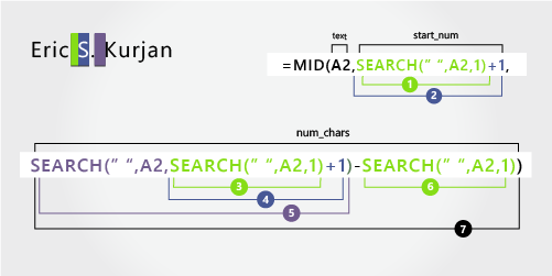
‘=MID(A2,SEARCH(» «,A2,1)+1,SEARCH(» «,A2,SEARCH(» «,A2,1)+1)-SEARCH(» «,A2,1)) |
=MID(A2,SEARCH(» «,A2,1)+1,SEARCH(» «,A2,SEARCH(» «,A2,1)+1)-SEARCH(» «,A2,1)) |
|
Formula |
Live Result (last name) |
|
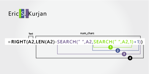
‘=RIGHT(A2,LEN(A2)-SEARCH(» «,A2,SEARCH(» «,A2,1)+1)) |
=RIGHT(A2,LEN(A2)-SEARCH(» «,A2,SEARCH(» «,A2,1)+1)) |
-
First name
The first name starts with the first character from the left (E) and ends at the fifth character (the first space). The formula extracts the first five characters in A2, starting from the left.
Use the SEARCH function to find the value for num_chars:
Search for the numeric position of the space in A2, starting from the left. (5)
-
Middle name
The middle name starts at the sixth character position (S), and ends at the eighth position (the second space). This formula involves nesting SEARCH functions to find the second instance of a space.
The formula extracts three characters, starting from the sixth position.
Use the SEARCH function to find the value for start_num:
Search for the numeric position of the first space in A2, starting from the first character from the left. (5).
-
Add 1 to get the position of the character after the first space (S). This numeric position is the starting position of the middle name. (5 + 1 = 6)
Use nested SEARCH functions to find the value for num_chars:
Search for the numeric position of the first space in A2, starting from the first character from the left. (5)
-
Add 1 to get the position of the character after the first space (S). The result is the character number at which you want to start searching for the second instance of space. (5 + 1 = 6)
-
Search for the second instance of space in A2, starting from the sixth position (S) found in step 4. This character number is the ending position of the middle name. (8)
-
Search for the numeric position of space in A2, starting from the first character from the left. (5)
-
Take the character number of the second space found in step 5 and subtract the character number of the first space found in step 6. The result is the number of characters MID extracts from the text string starting at the sixth position found in step 2. (8 – 5 = 3)
-
Last name
The last name starts six characters from the right (K) and ends at the first character from the right (n). This formula involves nesting SEARCH functions to find the second and third instances of a space (which are at the fifth and eighth positions from the left).
The formula extracts six characters in A2, starting from the right.
-
Use the LEN and nested SEARCH functions to find the value for num_chars:
Search for the numeric position of space in A2, starting from the first character from the left. (5)
-
Add 1 to get the position of the character after the first space (S). The result is the character number at which you want to start searching for the second instance of space. (5 + 1 = 6)
-
Search for the second instance of space in A2, starting from the sixth position (S) found in step 2. This character number is the ending position of the middle name. (8)
-
Count the total length of the text string in A2, and then subtract the number of characters from the left up to the second instance of space found in step 3. The result is the number of characters to be extracted from the right of the full name. (14 – 8 = 6).

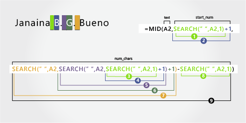
Here’s an example of how to extract two middle initials. The first and third instances of space separate the name components.
Copy the cells in the table and paste into an Excel worksheet at cell A1. The formula you see on the left will be displayed for reference, while Excel will automatically convert the formula on the right into the appropriate result.
Hint Before you paste the data into the worksheet, set the column widths of columns A and B to 250.
|
Example name |
Description |
|
Janaina B. G. Bueno |
Two middle initials |
|
Formula |
Result (first name) |
|
‘=LEFT(A2, SEARCH(» «,A2,1)) |
=LEFT(A2, SEARCH(» «,A2,1)) |
|
Formula |
Result (middle initials) |
|
‘=MID(A2,SEARCH(» «,A2,1)+1,SEARCH(» «,A2,SEARCH(» «,A2,SEARCH(» «,A2,1)+1)+1)-SEARCH(» «,A2,1)) |
=MID(A2,SEARCH(» «,A2,1)+1,SEARCH(» «,A2,SEARCH(» «,A2,SEARCH(» «,A2,1)+1)+1)-SEARCH(» «,A2,1)) |
|
Formula |
Live Result (last name) |
|
‘=RIGHT(A2,LEN(A2)-SEARCH(» «,A2,SEARCH(» «,A2,SEARCH(» «,A2,1)+1)+1)) |
=RIGHT(A2,LEN(A2)-SEARCH(» «,A2,SEARCH(» «,A2,SEARCH(» «,A2,1)+1)+1)) |
-
First name
The first name starts with the first character from the left (J) and ends at the eighth character (the first space). The formula extracts the first eight characters in A2, starting from the left.
Use the SEARCH function to find the value for num_chars:
Search for the numeric position of the first space in A2, starting from the left. (8)
-
Middle name
The middle name starts at the ninth position (B), and ends at the fourteenth position (the third space). This formula involves nesting SEARCH to find the first, second, and third instances of space in the eighth, eleventh, and fourteenth positions.
The formula extracts five characters, starting from the ninth position.
Use the SEARCH function to find the value for start_num:
Search for the numeric position of the first space in A2, starting from the first character from the left. (8)
-
Add 1 to get the position of the character after the first space (B). This numeric position is the starting position of the middle name. (8 + 1 = 9)
Use nested SEARCH functions to find the value for num_chars:
Search for the numeric position of the first space in A2, starting from the first character from the left. (8)
-
Add 1 to get the position of the character after the first space (B). The result is the character number at which you want to start searching for the second instance of space. (8 + 1 = 9)
-
Search for the second space in A2, starting from the ninth position (B) found in step 4. (11).
-
Add 1 to get the position of the character after the second space (G). This character number is the starting position at which you want to start searching for the third space. (11 + 1 = 12)
-
Search for the third space in A2, starting at the twelfth position found in step 6. (14)
-
Search for the numeric position of the first space in A2. (8)
-
Take the character number of the third space found in step 7 and subtract the character number of the first space found in step 6. The result is the number of characters MID extracts from the text string starting at the ninth position found in step 2.
-
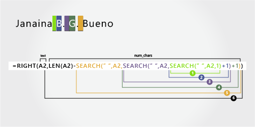
Last name
The last name starts five characters from the right (B) and ends at the first character from the right (o). This formula involves nesting SEARCH to find the first, second, and third instances of space.
The formula extracts five characters in A2, starting from the right of the full name.
Use nested SEARCH and the LEN functions to find the value for the num_chars:
Search for the numeric position of the first space in A2, starting from the first character from the left. (8)
-
Add 1 to get the position of the character after the first space (B). The result is the character number at which you want to start searching for the second instance of space. (8 + 1 = 9)
-
Search for the second space in A2, starting from the ninth position (B) found in step 2. (11)
-
Add 1 to get the position of the character after the second space (G). This character number is the starting position at which you want to start searching for the third instance of space. (11 + 1 = 12)
-
Search for the third space in A2, starting at the twelfth position (G) found in step 6. (14)
-
Count the total length of the text string in A2, and then subtract the number of characters from the left up to the third space found in step 5. The result is the number of characters to be extracted from the right of the full name. (19 — 14 = 5)

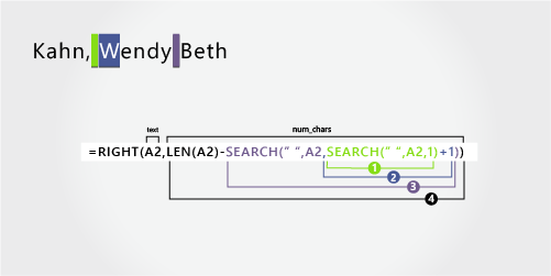
In this example, the last name comes before the first, and the middle name appears at the end. The comma marks the end of the last name, and a space separates each name component.
Copy the cells in the table and paste into an Excel worksheet at cell A1. The formula you see on the left will be displayed for reference, while Excel will automatically convert the formula on the right into the appropriate result.
Hint Before you paste the data into the worksheet, set the column widths of columns A and B to 250.
|
Example name |
Description |
|
Kahn, Wendy Beth |
Last name first, with comma |
|
Formula |
Result (first name) |
|
‘=MID(A2,SEARCH(» «,A2,1)+1,SEARCH(» «,A2,SEARCH(» «,A2,1)+1)-SEARCH(» «,A2,1)) |
=MID(A2,SEARCH(» «,A2,1)+1,SEARCH(» «,A2,SEARCH(» «,A2,1)+1)-SEARCH(» «,A2,1)) |
|
Formula |
Result (middle name) |
|
‘=RIGHT(A2,LEN(A2)-SEARCH(» «,A2,SEARCH(» «,A2,1)+1)) |
=RIGHT(A2,LEN(A2)-SEARCH(» «,A2,SEARCH(» «,A2,1)+1)) |
|
Formula |
Live Result (last name) |
|
‘=LEFT(A2, SEARCH(» «,A2,1)-2) |
=LEFT(A2, SEARCH(» «,A2,1)-2) |
-
First name
The first name starts with the seventh character from the left (W) and ends at the twelfth character (the second space). Because the first name occurs at the middle of the full name, you need to use the MID function to extract the first name.
The formula extracts six characters, starting from the seventh position.
Use the SEARCH function to find the value for start_num:
Search for the numeric position of the first space in A2, starting from the first character from the left. (6)
-
Add 1 to get the position of the character after the first space (W). This numeric position is the starting position of the first name. (6 + 1 = 7)
Use nested SEARCH functions to find the value for num_chars:
Search for the numeric position of the first space in A2, starting from the first character from the left. (6)
-
Add 1 to get the position of the character after the first space (W). The result is the character number at which you want to start searching for the second space. (6 + 1 = 7)
Search for the second space in A2, starting from the seventh position (W) found in step 4. (12)
-
Search for the numeric position of the first space in A2, starting from the first character from the left. (6)
-
Take the character number of the second space found in step 5 and subtract the character number of the first space found in step 6. The result is the number of characters MID extracts from the text string starting at the seventh position found in step 2. (12 — 6 = 6)
-
Middle name
The middle name starts four characters from the right (B), and ends at the first character from the right (h). This formula involves nesting SEARCH to find the first and second instances of space in the sixth and twelfth positions from the left.
The formula extracts four characters, starting from the right.
Use nested SEARCH and the LEN functions to find the value for start_num:
Search for the numeric position of the first space in A2, starting from the first character from the left. (6)
-
Add 1 to get the position of the character after the first space (W). The result is the character number at which you want to start searching for the second space. (6 + 1 = 7)
-
Search for the second instance of space in A2 starting from the seventh position (W) found in step 2. (12)
-
Count the total length of the text string in A2, and then subtract the number of characters from the left up to the second space found in step 3. The result is the number of characters to be extracted from the right of the full name. (16 — 12 = 4)
-
Last name
The last name starts with the first character from the left (K) and ends at the fourth character (n). The formula extracts four characters, starting from the left.
Use the SEARCH function to find the value for num_chars:
Search for the numeric position of the first space in A2, starting from the first character from the left. (6)
-
Subtract 2 to get the numeric position of the ending character of the last name (n). The result is the number of characters you want LEFT to extract. (6 — 2 =4)


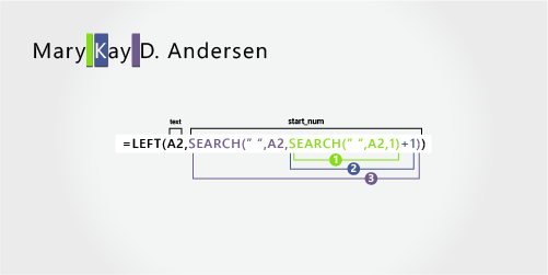
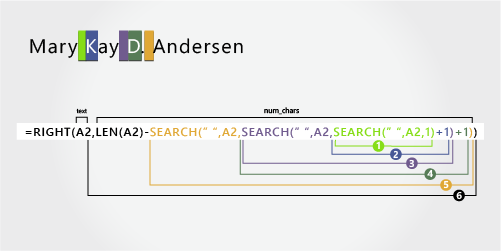
This example uses a two-part first name, Mary Kay. The second and third spaces separate each name component.
Copy the cells in the table and paste into an Excel worksheet at cell A1. The formula you see on the left will be displayed for reference, while Excel will automatically convert the formula on the right into the appropriate result.
Hint Before you paste the data into the worksheet, set the column widths of columns A and B to 250.
|
Example name |
Description |
|
Mary Kay D. Andersen |
Two-part first name |
|
Formula |
Result (first name) |
|
LEFT(A2, SEARCH(» «,A2,SEARCH(» «,A2,1)+1)) |
=LEFT(A2, SEARCH(» «,A2,SEARCH(» «,A2,1)+1)) |
|
Formula |
Result (middle initial) |
|
‘=MID(A2,SEARCH(» «,A2,SEARCH(» «,A2,1)+1)+1,SEARCH(» «,A2,SEARCH(» «,A2,SEARCH(» «,A2,1)+1)+1)-(SEARCH(» «,A2,SEARCH(» «,A2,1)+1)+1)) |
=MID(A2,SEARCH(» «,A2,SEARCH(» «,A2,1)+1)+1,SEARCH(» «,A2,SEARCH(» «,A2,SEARCH(» «,A2,1)+1)+1)-(SEARCH(» «,A2,SEARCH(» «,A2,1)+1)+1)) |
|
Formula |
Live Result (last name) |
|
‘=RIGHT(A2,LEN(A2)-SEARCH(» «,A2,SEARCH(» «,A2,SEARCH(» «,A2,1)+1)+1)) |
=RIGHT(A2,LEN(A2)-SEARCH(» «,A2,SEARCH(» «,A2,SEARCH(» «,A2,1)+1)+1)) |
-
First name
The first name starts with the first character from the left and ends at the ninth character (the second space). This formula involves nesting SEARCH to find the second instance of space from the left.
The formula extracts nine characters, starting from the left.
Use nested SEARCH functions to find the value for num_chars:
Search for the numeric position of the first space in A2, starting from the first character from the left. (5)
-
Add 1 to get the position of the character after the first space (K). The result is the character number at which you want to start searching for the second instance of space. (5 + 1 = 6)
-
Search for the second instance of space in A2, starting from the sixth position (K) found in step 2. The result is the number of characters LEFT extracts from the text string. (9)
-
Middle name
The middle name starts at the tenth position (D), and ends at the twelfth position (the third space). This formula involves nesting SEARCH to find the first, second, and third instances of space.
The formula extracts two characters from the middle, starting from the tenth position.
Use nested SEARCH functions to find the value for start_num:
Search for the numeric position of the first space in A2, starting from the first character from the left. (5)
-
Add 1 to get the character after the first space (K). The result is the character number at which you want to start searching for the second space. (5 + 1 = 6)
-
Search for the position of the second instance of space in A2, starting from the sixth position (K) found in step 2. The result is the number of characters LEFT extracts from the left. (9)
-
Add 1 to get the character after the second space (D). The result is the starting position of the middle name. (9 + 1 = 10)
Use nested SEARCH functions to find the value for num_chars:
Search for the numeric position of the character after the second space (D). The result is the character number at which you want to start searching for the third space. (10)
-
Search for the numeric position of the third space in A2, starting from the left. The result is the ending position of the middle name. (12)
-
Search for the numeric position of the character after the second space (D). The result is the beginning position of the middle name. (10)
-
Take the character number of the third space, found in step 6, and subtract the character number of “D”, found in step 7. The result is the number of characters MID extracts from the text string starting at the tenth position found in step 4. (12 — 10 = 2)
-
Last name
The last name starts eight characters from the right. This formula involves nesting SEARCH to find the first, second, and third instances of space in the fifth, ninth, and twelfth positions.
The formula extracts eight characters from the right.
Use nested SEARCH and the LEN functions to find the value for num_chars:
Search for the numeric position of the first space in A2, starting from the left. (5)
-
Add 1 to get the character after the first space (K). The result is the character number at which you want to start searching for the space. (5 + 1 = 6)
-
Search for the second space in A2, starting from the sixth position (K) found in step 2. (9)
-
Add 1 to get the position of the character after the second space (D). The result is the starting position of the middle name. (9 + 1 = 10)
-
Search for the numeric position of the third space in A2, starting from the left. The result is the ending position of the middle name. (12)
-
Count the total length of the text string in A2, and then subtract the number of characters from the left up to the third space found in step 5. The result is the number of characters to be extracted from the right of the full name. (20 — 12 =


This example uses a three-part last name: Barreto de Mattos. The first space marks the end of the first name and the beginning of the last name.
Copy the cells in the table and paste into an Excel worksheet at cell A1. The formula you see on the left will be displayed for reference, while Excel will automatically convert the formula on the right into the appropriate result.
Hint Before you paste the data into the worksheet, set the column widths of columns A and B to 250.
|
Example name |
Description |
|
Paula Barreto de Mattos |
Three-part last name |
|
Formula |
Result (first name) |
|
‘=LEFT(A2, SEARCH(» «,A2,1)) |
=LEFT(A2, SEARCH(» «,A2,1)) |
|
Formula |
Result (last name) |
|
RIGHT(A2,LEN(A2)-SEARCH(» «,A2,1)) |
=RIGHT(A2,LEN(A2)-SEARCH(» «,A2,1)) |
-
First name
The first name starts with the first character from the left (P) and ends at the sixth character (the first space). The formula extracts six characters from the left.
Use the Search function to find the value for num_chars:
Search for the numeric position of the first space in A2, starting from the left. (6)
-
Last name
The last name starts seventeen characters from the right (B) and ends with first character from the right (s). The formula extracts seventeen characters from the right.
Use the LEN and SEARCH functions to find the value for num_chars:
Search for the numeric position of the first space in A2, starting from the left. (6)
-
Count the total length of the text string in A2, and then subtract the number of characters from the left up to the first space, found in step 1. The result is the number of characters to be extracted from the right of the full name. (23 — 6 = 17)


This example uses a two-part last name: van Eaton. The first space marks the end of the first name and the beginning of the last name.
Copy the cells in the table and paste into an Excel worksheet at cell A1. The formula you see on the left will be displayed for reference, while Excel will automatically convert the formula on the right into the appropriate result.
Hint Before you paste the data into the worksheet, set the column widths of columns A and B to 250.
|
Example name |
Description |
|
James van Eaton |
Two-part last name |
|
Formula |
Result (first name) |
|
‘=LEFT(A2, SEARCH(» «,A2,1)) |
=LEFT(A2, SEARCH(» «,A2,1)) |
|
Formula |
Result (last name) |
|
‘=RIGHT(A2,LEN(A2)-SEARCH(» «,A2,1)) |
=RIGHT(A2,LEN(A2)-SEARCH(» «,A2,1)) |
-
First name
The first name starts with the first character from the left (J) and ends at the eighth character (the first space). The formula extracts six characters from the left.
Use the SEARCH function to find the value for num_chars:
Search for the numeric position of the first space in A2, starting from the left. (6)
-
Last name
The last name starts with the ninth character from the right (v) and ends at the first character from the right (n). The formula extracts nine characters from the right of the full name.
Use the LEN and SEARCH functions to find the value for num_chars:
Search for the numeric position of the first space in A2, starting from the left. (6)
-
Count the total length of the text string in A2, and then subtract the number of characters from the left up to the first space, found in step 1. The result is the number of characters to be extracted from the right of the full name. (15 — 6 = 9)


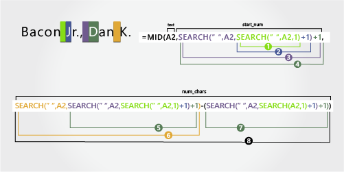
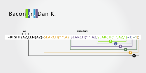
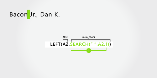
In this example, the last name comes first, followed by the suffix. The comma separates the last name and suffix from the first name and middle initial.
Copy the cells in the table and paste into an Excel worksheet at cell A1. The formula you see on the left will be displayed for reference, while Excel will automatically convert the formula on the right into the appropriate result.
Hint Before you paste the data into the worksheet, set the column widths of columns A and B to 250.
|
Example name |
Description |
|
Bacon Jr., Dan K. |
Last name and suffix first, with comma |
|
Formula |
Result (first name) |
|
‘=MID(A2,SEARCH(» «,A2,SEARCH(» «,A2,1)+1)+1,SEARCH(» «,A2,SEARCH(» «,A2,SEARCH(» «,A2,1)+1)+1)-SEARCH(» «,A2,SEARCH(» «,A2,1)+1)) |
=MID(A2,SEARCH(» «,A2,SEARCH(» «,A2,1)+1)+1,SEARCH(» «,A2,SEARCH(» «,A2,SEARCH(» «,A2,1)+1)+1)-SEARCH(» «,A2,SEARCH(» «,A2,1)+1)) |
|
Formula |
Result (middle initial) |
|
‘=RIGHT(A2,LEN(A2)-SEARCH(» «,A2,SEARCH(» «,A2,SEARCH(» «,A2,1)+1)+1)) |
=RIGHT(A2,LEN(A2)-SEARCH(» «,A2,SEARCH(» «,A2,SEARCH(» «,A2,1)+1)+1)) |
|
Formula |
Result (last name) |
|
‘=LEFT(A2, SEARCH(» «,A2,1)) |
=LEFT(A2, SEARCH(» «,A2,1)) |
|
Formula |
Result (suffix) |
|
‘=MID(A2,SEARCH(» «, A2,1)+1,(SEARCH(» «,A2,SEARCH(» «,A2,1)+1)-2)-SEARCH(» «,A2,1)) |
=MID(A2,SEARCH(» «, A2,1)+1,(SEARCH(» «,A2,SEARCH(» «,A2,1)+1)-2)-SEARCH(» «,A2,1)) |
-
First name
The first name starts with the twelfth character (D) and ends with the fifteenth character (the third space). The formula extracts three characters, starting from the twelfth position.
Use nested SEARCH functions to find the value for start_num:
Search for the numeric position of the first space in A2, starting from the left. (6)
-
Add 1 to get the character after the first space (J). The result is the character number at which you want to start searching for the second space. (6 + 1 = 7)
-
Search for the second space in A2, starting from the seventh position (J), found in step 2. (11)
-
Add 1 to get the character after the second space (D). The result is the starting position of the first name. (11 + 1 = 12)
Use nested SEARCH functions to find the value for num_chars:
Search for the numeric position of the character after the second space (D). The result is the character number at which you want to start searching for the third space. (12)
-
Search for the numeric position of the third space in A2, starting from the left. The result is the ending position of the first name. (15)
-
Search for the numeric position of the character after the second space (D). The result is the beginning position of the first name. (12)
-
Take the character number of the third space, found in step 6, and subtract the character number of “D”, found in step 7. The result is the number of characters MID extracts from the text string starting at the twelfth position, found in step 4. (15 — 12 = 3)
-
Middle name
The middle name starts with the second character from the right (K). The formula extracts two characters from the right.
Search for the numeric position of the first space in A2, starting from the left. (6)
-
Add 1 to get the character after the first space (J). The result is the character number at which you want to start searching for the second space. (6 + 1 = 7)
-
Search for the second space in A2, starting from the seventh position (J), found in step 2. (11)
-
Add 1 to get the character after the second space (D). The result is the starting position of the first name. (11 + 1 = 12)
-
Search for the numeric position of the third space in A2, starting from the left. The result is the ending position of the middle name. (15)
-
Count the total length of the text string in A2, and then subtract the number of characters from the left up to the third space, found in step 5. The result is the number of characters to be extracted from the right of the full name. (17 — 15 = 2)
-
Last name
The last name starts at the first character from the left (B) and ends at sixth character (the first space). Therefore, the formula extracts six characters from the left.
Use the SEARCH function to find the value for num_chars:
Search for the numeric position of the first space in A2, starting from the left. (6)
-
Suffix
The suffix starts at the seventh character from the left (J), and ends at ninth character from the left (.). The formula extracts three characters, starting from the seventh character.
Use the SEARCH function to find the value for start_num:
Search for the numeric position of the first space in A2, starting from the left. (6)
-
Add 1 to get the character after the first space (J). The result is the starting position of the suffix. (6 + 1 = 7)
Use nested SEARCH functions to find the value for num_chars:
Search for the numeric position of the first space in A2, starting from the left. (6)
-
Add 1 to get the numeric position of the character after the first space (J). The result is the character number at which you want to start searching for the second space. (7)
-
Search for the numeric position of the second space in A2, starting from the seventh character found in step 4. (11)
-
Subtract 1 from the character number of the second space found in step 4 to get the character number of “,”. The result is the ending position of the suffix. (11 — 1 = 10)
-
Search for the numeric position of the first space. (6)
-
After finding the first space, add 1 to find the next character (J), also found in steps 3 and 4. (7)
-
Take the character number of “,” found in step 6, and subtract the character number of “J”, found in steps 3 and 4. The result is the number of characters MID extracts from the text string starting at the seventh position, found in step 2. (10 — 7 = 3)

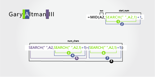
In this example, the first name is at the beginning of the string and the suffix is at the end, so you can use formulas similar to Example 2: Use the LEFT function to extract the first name, the MID function to extract the last name, and the RIGHT function to extract the suffix.
Copy the cells in the table and paste into an Excel worksheet at cell A1. The formula you see on the left will be displayed for reference, while Excel will automatically convert the formula on the right into the appropriate result.
Hint Before you paste the data into the worksheet, set the column widths of columns A and B to 250.
|
Example name |
Description |
|
Gary Altman III |
First and last name with suffix |
|
Formula |
Result (first name) |
|
‘=LEFT(A2, SEARCH(» «,A2,1)) |
=LEFT(A2, SEARCH(» «,A2,1)) |
|
Formula |
Result (last name) |
|
‘=MID(A2,SEARCH(» «,A2,1)+1,SEARCH(» «,A2,SEARCH(» «,A2,1)+1)-(SEARCH(» «,A2,1)+1)) |
=MID(A2,SEARCH(» «,A2,1)+1,SEARCH(» «,A2,SEARCH(» «,A2,1)+1)-(SEARCH(» «,A2,1)+1)) |
|
Formula |
Result (suffix) |
|
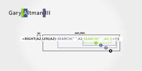
‘=RIGHT(A2,LEN(A2)-SEARCH(» «,A2,SEARCH(» «,A2,1)+1)) |
=RIGHT(A2,LEN(A2)-SEARCH(» «,A2,SEARCH(» «,A2,1)+1)) |
-
First name
The first name starts at the first character from the left (G) and ends at the fifth character (the first space). Therefore, the formula extracts five characters from the left of the full name.
Search for the numeric position of the first space in A2, starting from the left. (5)
-
Last name
The last name starts at the sixth character from the left (A) and ends at the eleventh character (the second space). This formula involves nesting SEARCH to find the positions of the spaces.
The formula extracts six characters from the middle, starting from the sixth character.
Use the SEARCH function to find the value for start_num:
Search for the numeric position of the first space in A2, starting from the left. (5)
-
Add 1 to get the position of the character after the first space (A). The result is the starting position of the last name. (5 + 1 = 6)
Use nested SEARCH functions to find the value for num_chars:
Search for the numeric position of the first space in A2, starting from the left. (5)
-
Add 1 to get the position of the character after the first space (A). The result is the character number at which you want to start searching for the second space. (5 + 1 = 6)
-
Search for the numeric position of the second space in A2, starting from the sixth character found in step 4. This character number is the ending position of the last name. (12)
-
Search for the numeric position of the first space. (5)
-
Add 1 to find the numeric position of the character after the first space (A), also found in steps 3 and 4. (6)
-
Take the character number of the second space, found in step 5, and then subtract the character number of “A”, found in steps 6 and 7. The result is the number of characters MID extracts from the text string, starting at the sixth position, found in step 2. (12 — 6 = 6)
-
Suffix
The suffix starts three characters from the right. This formula involves nesting SEARCH to find the positions of the spaces.
Use nested SEARCH and the LEN functions to find the value for num_chars:
Search for the numeric position of the first space in A2, starting from the left. (5)
-
Add 1 to get the character after the first space (A). The result is the character number at which you want to start searching for the second space. (5 + 1 = 6)
-
Search for the second space in A2, starting from the sixth position (A), found in step 2. (12)
-
Count the total length of the text string in A2, and then subtract the number of characters from the left up to the second space, found in step 3. The result is the number of characters to be extracted from the right of the full name. (15 — 12 = 3)

In this example, the full name is preceded by a prefix, and you use formulas similar to Example 2: the MID function to extract the first name, the RIGHT function to extract the last name.
Copy the cells in the table and paste into an Excel worksheet at cell A1. The formula you see on the left will be displayed for reference, while Excel will automatically convert the formula on the right into the appropriate result.
Hint Before you paste the data into the worksheet, set the column widths of columns A and B to 250.
|
Example name |
Description |
|
Mr. Ryan Ihrig |
With prefix |
|
Formula |
Result (first name) |
|
‘=MID(A2,SEARCH(» «,A2,1)+1,SEARCH(» «,A2,SEARCH(» «,A2,1)+1)-(SEARCH(» «,A2,1)+1)) |
=MID(A2,SEARCH(» «,A2,1)+1,SEARCH(» «,A2,SEARCH(» «,A2,1)+1)-(SEARCH(» «,A2,1)+1)) |
|
Formula |
Result (last name) |
|
‘=RIGHT(A2,LEN(A2)-SEARCH(» «,A2,SEARCH(» «,A2,1)+1)) |
=RIGHT(A2,LEN(A2)-SEARCH(» «,A2,SEARCH(» «,A2,1)+1)) |
-
First name
The first name starts at the fifth character from the left (R) and ends at the ninth character (the second space). The formula nests SEARCH to find the positions of the spaces. It extracts four characters, starting from the fifth position.
Use the SEARCH function to find the value for the start_num:
Search for the numeric position of the first space in A2, starting from the left. (4)
-
Add 1 to get the position of the character after the first space (R). The result is the starting position of the first name. (4 + 1 = 5)
Use nested SEARCH function to find the value for num_chars:
Search for the numeric position of the first space in A2, starting from the left. (4)
-
Add 1 to get the position of the character after the first space (R). The result is the character number at which you want to start searching for the second space. (4 + 1 = 5)
-
Search for the numeric position of the second space in A2, starting from the fifth character, found in steps 3 and 4. This character number is the ending position of the first name. (9)
-
Search for the first space. (4)
-
Add 1 to find the numeric position of the character after the first space (R), also found in steps 3 and 4. (5)
-
Take the character number of the second space, found in step 5, and then subtract the character number of “R”, found in steps 6 and 7. The result is the number of characters MID extracts from the text string, starting at the fifth position found in step 2. (9 — 5 = 4)
-
Last name
The last name starts five characters from the right. This formula involves nesting SEARCH to find the positions of the spaces.
Use nested SEARCH and the LEN functions to find the value for num_chars:
Search for the numeric position of the first space in A2, starting from the left. (4)
-
Add 1 to get the position of the character after the first space (R). The result is the character number at which you want to start searching for the second space. (4 + 1 = 5)
-
Search for the second space in A2, starting from the fifth position (R), found in step 2. (9)
-
Count the total length of the text string in A2, and then subtract the number of characters from the left up to the second space, found in step 3. The result is the number of characters to be extracted from the right of the full name. (14 — 9 = 5)


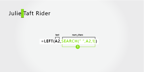
This example uses a hyphenated last name. A space separates each name component.
Copy the cells in the table and paste into an Excel worksheet at cell A1. The formula you see on the left will be displayed for reference, while Excel will automatically convert the formula on the right into the appropriate result.
Hint Before you paste the data into the worksheet, set the column widths of columns A and B to 250.
|
Example name |
Description |
|
Julie Taft-Rider |
Hyphenated last name |
|
Formula |
Result (first name) |
|
‘=LEFT(A2, SEARCH(» «,A2,1)) |
=LEFT(A2, SEARCH(» «,A2,1)) |
|
Formula |
Result (last name) |
|
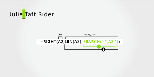
‘=RIGHT(A2,LEN(A2)-SEARCH(» «,A2,1)) |
=RIGHT(A2,LEN(A2)-SEARCH(» «,A2,1)) |
-
First name
The first name starts at the first character from the left and ends at the sixth position (the first space). The formula extracts six characters from the left.
Use the SEARCH function to find the value of num_chars:
Search for the numeric position of the first space in A2, starting from the left. (6)
-
Last name
The entire last name starts ten characters from the right (T) and ends at the first character from the right (r).
Use the LEN and SEARCH functions to find the value for num_chars:
Search for the numeric position of the space in A2, starting from the first character from the left. (6)
-
Count the total length of the text string to be extracted, and then subtract the number of characters from the left up to the first space, found in step 1. (16 — 6 = 10)
Need more help?
Want more options?
Explore subscription benefits, browse training courses, learn how to secure your device, and more.
Communities help you ask and answer questions, give feedback, and hear from experts with rich knowledge.
One scenario is where you need to join multiple strings of text into a single text string. The flip of that is splitting a single text string into multiple text strings. If the data at hand was copied from somewhere or created by someone who completely missed the point of Excel columns, you will find that you need to split a block of text to categorize it.
Splitting the text largely depends on the delimiter in the text string. A delimiter is a character or symbol that marks the beginning or end of a character string. Examples of a delimiter are a space character, hyphen, period, comma.
 1")
Our example case for this guide involves splitting book details into book title, author, and genre. The delimiter we’ve used is a comma:
 2")
This tutorial will teach you how to split text in Excel with the Text to Columns and Flash Fill features, formulas, and VBA. The formulas method includes splitting text by a specific character. That’s the menu today.
Let’s get splitting!
Using Text to Columns
This feature lives up to its name. Text to Columns splits a column of text into multiple columns with specified controls. Text to Columns can split text with delimiters and since our data contains only a comma as the delimiter, using the feature becomes very easy. See the following steps to split text using Text to Columns:
- Select the data you want to split.
- Go to the Data tab and select the Text to Columns icon from the Data Tools
 3")
- Select the Delimited radio button and then click on the Next
 4")
- In the Delimiters section, select the Comma
- Then select the Next button.
 5")
- Now you need to choose where you want the split text. Click on the Destination field, then select the destination cell on the worksheet in the background where you want the split text to start.
- Select the Finish button to close the Text to Columns
 6")
Using the comma delimiter to separate the text string, Text to Columns has split the text from our example case into three columns:
 7")
Luckily, our data doesn’t contain a book with commas in the book name. If we had the book Cows, Pigs, Wars and Witches by Marvin Harris in the dataset, the text would be split into 5 columns instead of 3 like the rest. If the delimiter in your data is appearing in the text string for more than delimiting, you’ll have better luck splitting text with other methods. Now unto another observation.
Using TRIM Function to Trim Extra Spaces
Let’s cast a closer look at the output of Text to Columns. Notice how the last two columns carry one leading space? You can see that the values in columns D and E are not a hundred percent aligned to the left:
 8")
The last two columns carry a leading space because Text to Columns only takes the delimiter as a mark from where to split the text. The space character after the comma is carried with the next unit of text and that has our data with a leading space.
A quick fix for this is to use the TRIM function to clear up extra spaces. Here is the formula we have used to remove leading spaces from columns D and E:
=TRIM(C4)
The TRIM function removes all spaces from a text string other than a single space character between two words. Any leading, trailing, or extra spaces will be removed from the cell’s value. We have simply used the formula with a reference of the cell containing the leading space.
And that cleaned up the leading spaces for us. Data – good to go!
 9")
Using Formula To Separate Text in Excel
We can make use to Excel functions to construct formulas that can help us in splitting a text string into multiple.
Split String with Delimiter
Using a formula can also split a single text string into multiple strings but it will require a combo of functions. Let’s have a little briefing on the functions that make part of this formula we will use for splitting text.
The SUBSTITUTE function replaces old text in a text string with new text.
The REPT function repeats text a given number of times.
The LEN function returns the number of characters in a text string.
The MID function returns a given number of characters from the middle of a text string with a specified starting position.
The TRIM function removes all spaces, other than single spaces between words, from a text string.
Now let’s see how these functions combined can be used to split text with a single formula:
=TRIM(MID(SUBSTITUTE($B5,",",REPT(" ",LEN($B5))),(C$4-1)*LEN($B5)+1,LEN($B5)))
In our example, the first cell we are using this formula on is cell B5. The number of characters in B5 as counted by the LEN function is 49. The REPT function repeats spaces (denoted by “ “ in the formula) in B5 for the number of characters supplied by the LEN function i.e. 49.
The SUBSTITUTE function replaces the commas “,” in B5 with 49 space characters supplied by the REPT function. Since there are two commas in B5, one after the book name and one after the author, 49 spaces will be entered after the book name and 49 spaces after the author, creating a decent gap between the text we want to split.
Now let’s see the calculations for the MID function. The first bit is (C$4-1). In row 4, we added serial numbering for each of the columns for our categories. The row has been locked in the formula with a $ sign so the row doesn’t change as the formula is copied down. But we have left the column free so that the serial number changes for the respective columns used in the formula.
In the formula, 1 is subtracted from C4 (1-1=0) and the result is multiplied by the number of characters in B5 i.e. LEN($B5) and then 1 is added to the expression. The calculation for the starting position in the MID function, i.e. (C$4-1)*LEN($B5)+1, becomes (1-1)*49+1 which equals 1.
The MID function returns the text from the middle of B5, the starting position is 1 (that means the text to be returned is to start from the first character) and the number of characters to be returned is LEN($B5) i.e 49 characters. Since we have added 49 spaces in place of each of the commas, that gives us plenty of area to safely return just one chunk of text along with some extra spaces. The result up until the MID function is A Song of Ice and Fire with lots of trailing spaces.
The extra spaces are no problem. The TRIM function cleans any extra spaces leaving the single spaces between words and so we finally have the book name returned as A Song of Ice and Fire.
 10")
Now for the next column and hence the next category, the calculation for the starting position in the MID function will change like so (D$4-1)*LEN($B5)+1. The expression comes down to (2-1)*49+1 which equals 50. If the MID function is to return characters starting from the 50th character, with all the extra spaces added by the REPT function, what the MID function will return will be along this pattern: spaces author spaces.
The leading and trailing spaces will be trimmed by the TRIM function and the result will be George RR Martin.
 11")
The “+1” in the starting position argument of the MID function has no relevance for the subsequent columns, only for the first. That is because, without the “+1” in the first column’s calculation, it would be 0*49 which will end up in a #VALUE! error.
The formula copied along column E gives us the genre from the combined text in column B and that completes our set.
Split String at Specific Character
If there is only a single delimiter that is a specific character, such a lengthy formula as above will not be required to split the text. Let’s say, like our case example below, we are to split product code and product type which is joined by a hyphen.
Now this would be easier if the product code had a fixed number of characters; we would only have to use the LEFT function to return a certain number of characters. But what’s the fun in that?
We are going to let the FIND function do a bit of search work for us and find the hyphen in the text so the LEFT function and RIGHT function can return the surrounding text. This is the formula with the LEFT function for returning the first extract:
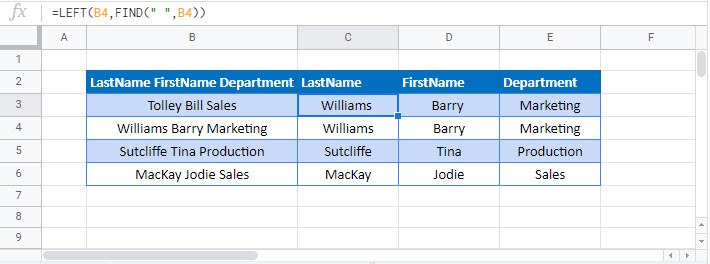
=LEFT(B3,FIND("-",B3)-1)
The FIND function searches B3 for the position of the hyphen “-“ in the text string, which is 6. The LEFT function then returns the characters starting from the left of the text and the number of characters to return is 6-1. “-1” at the end ensures that the characters returned do not include the hyphen itself. Here are the results of this formula for returning the first segment of split text:
 12")
Now for the second segment of text, the RIGHT function comes into play with this formula:
=RIGHT(B3,LEN(B3)-FIND("-",B3))
The FIND function is again used to find the location of the hyphen in B3 which we know is the 6th character. The LEN function returns the number of characters in B3 as 23. The RIGHT function extracts 23-6 characters from B3 and returns the product type “Bluetooth Speaker”. This is how it has worked for our example:
 13")
Using Flash Fill
The Flash Fill feature in Excel automatically fills in values based on a couple of manually provided examples. The ease of Flash Fill is that you need not remember any formulas, use any wizards, or fiddle with any settings. If your data is consistent, Flash Fill will be the quickest to pick up on what you are trying to get done. Let’s see the steps for using Flash Fill to split text and how it works for our example case:
- Type the first text as an example for Flash Fill to pick up the pattern and press the Enter
 14")
- From the Home tab’s Editing group, click on the Fill icon and select Flash Fill from the menu.
- Alternatively, use the shortcut keys Ctrl + E.
 15")
- Picking up on the provided example, Flash Fill will split the text and fill the column according to the same pattern:
 16")
- Repeat the same steps for each column to be Flash-Filled.
 17")
Flash Fill will save the trouble of having to trim leading and trailing spaces but as mentioned, if there are any anomalies or inconsistencies in the data (e.g a space before and after the comma), Flash Fill won’t be a reliable method of splitting text and due to the bulk of the data, the problem may go ignored. If you doubt the data to have inconsistencies, use the other methods for splitting the text.
Using VBA Function
The final method we will be discussing today for splitting text will be a VBA function. In order to automate tasks in MS Office applications, macros can be created and used with VBA. Our task is to split text in Excel and below are the steps for doing this using VBA:
- If you have the Developer tab added to the toolbar Ribbon, click on the Developer tab and then select the Visual Basic icon in the Code group to launch the Visual Basic
- You can also use the Alt + F11 keys.
 18")
- The Visual Basic editor will have opened:
 19")
- Open the Insert tab and select Module from the list. A Module window will open.
 20")
- In the Module window, copy-paste the following code to create a macro titled SplitText:
Sub SplitText()
Dim MyArray() As String, Count As Long, i As Variant
For n = 4 To 16
 MyArray = Split(Cells(n, 2), ",")
 Count = 3
 For Each i In MyArray
 Cells(n, Count) = i
 Count = Count + 1
 Next i
Next n
End Sub
Edit the following parts of the code as per your data:
- ‘For n = 4 To 16’ – 4 and 16 represent the first and last rows of the dataset.
- ‘MyArray = Split(Cells(n, 2), «,»)’ – The comma enclosed with double quotes is the delimiter.
- ‘Count = 3’ – 3 is the column number of the first column that the resulting data will be returned in.
 21")
- To run the code, press the F5
The data will be split as per the supplied values:
- Clean up the leading spaces in columns D and E using the TRIM function:
Now let’s split the active guide from its conclusion. Today you learned a few ways on how to split text in Excel. If you find yourself splitting hairs on your ability to split text next time, pocket this one and be ready to give it a go! We’ll be back with more Excel-ness to fill your pockets. Make some space!
Содержание
- Способ 1: Использование автоматического инструмента
- Способ 2: Создание формулы разделения текста
- Шаг 1: Разделение первого слова
- Шаг 2: Разделение второго слова
- Шаг 3: Разделение третьего слова
- Вопросы и ответы

Способ 1: Использование автоматического инструмента
В Excel есть автоматический инструмент, предназначенный для разделения текста по столбцам. Он не работает в автоматическом режиме, поэтому все действия придется выполнять вручную, предварительно выбирая диапазон обрабатываемых данных. Однако настройка является максимально простой и быстрой в реализации.
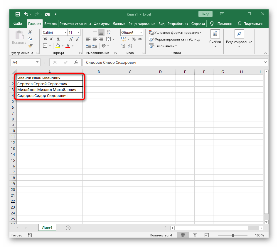
- С зажатой левой кнопкой мыши выделите все ячейки, текст которых хотите разделить на столбцы.
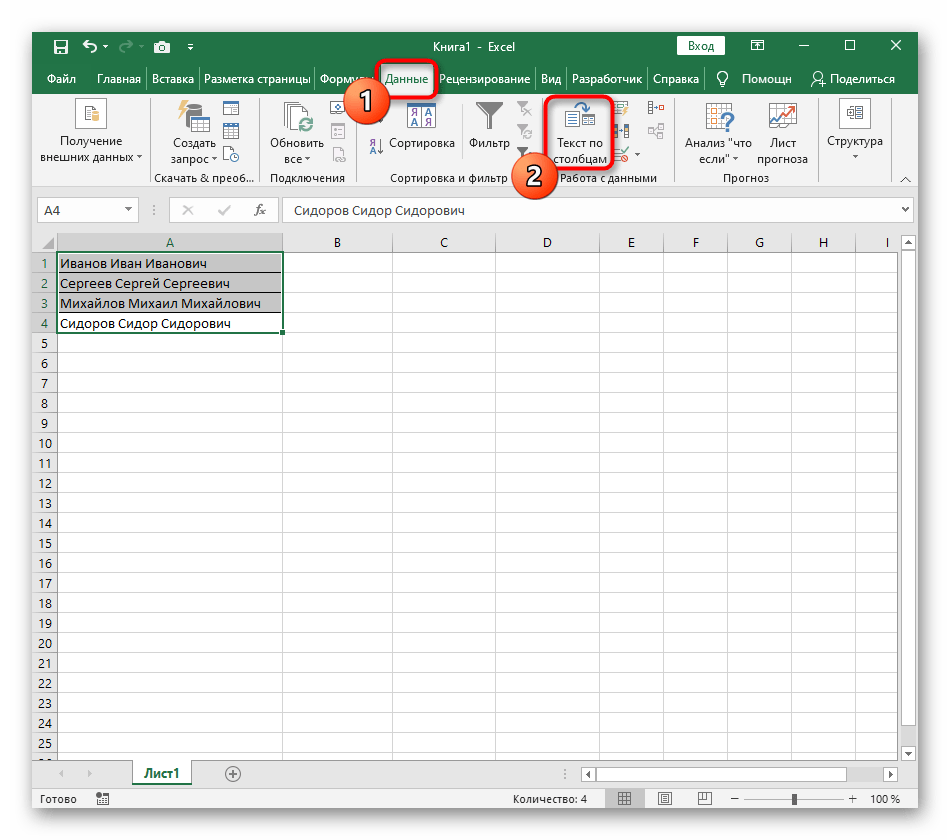
- После этого перейдите на вкладку «Данные» и нажмите кнопку «Текст по столбцам».
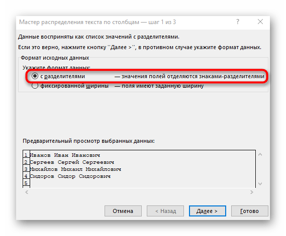
- Появится окно «Мастера разделения текста по столбцам», в котором нужно выбрать формат данных «с разделителями». Разделителем чаще всего выступает пробел, но если это другой знак препинания, понадобится указать его в следующем шаге.
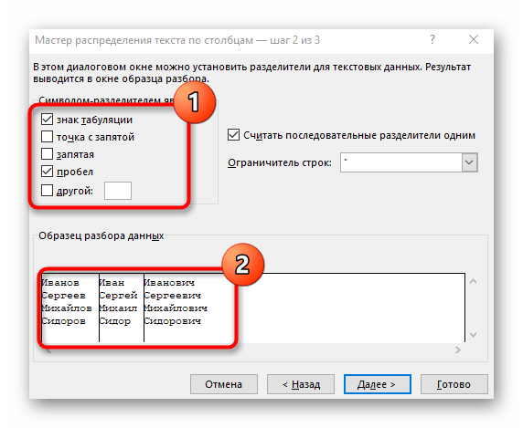
- Отметьте галочкой символ разделения или вручную впишите его, а затем ознакомьтесь с предварительным результатом разделения в окне ниже.
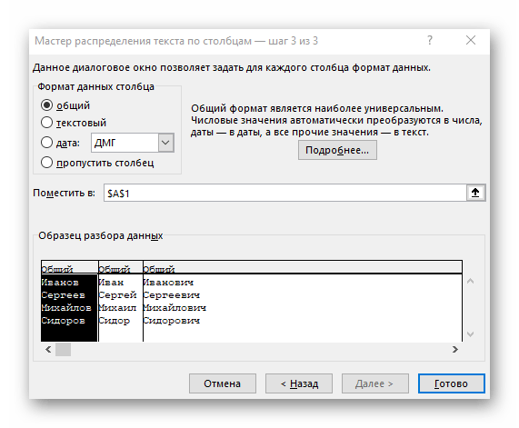
- В завершающем шаге можно указать новый формат столбцов и место, куда их необходимо поместить. Как только настройка будет завершена, нажмите «Готово» для применения всех изменения.
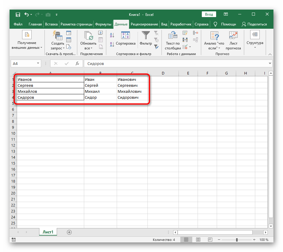
- Вернитесь к таблице и убедитесь в том, что разделение прошло успешно.
Из этой инструкции можно сделать вывод, что использование такого инструмента оптимально в тех ситуациях, когда разделение необходимо выполнить всего один раз, обозначив для каждого слова новый столбец. Однако если в таблицу постоянно вносятся новые данные, все время разделять их таким образом будет не совсем удобно, поэтому в таких случаях предлагаем ознакомиться со следующим способом.
Способ 2: Создание формулы разделения текста
В Excel можно самостоятельно создать относительно сложную формулу, которая позволит рассчитать позиции слов в ячейке, найти пробелы и разделить каждое на отдельные столбцы. В качестве примера мы возьмем ячейку, состоящую из трех слов, разделенных пробелами. Для каждого из них понадобится своя формула, поэтому разделим способ на три этапа.
Шаг 1: Разделение первого слова
Формула для первого слова самая простая, поскольку придется отталкиваться только от одного пробела для определения правильной позиции. Рассмотрим каждый шаг ее создания, чтобы сформировалась полная картина того, зачем нужны определенные вычисления.
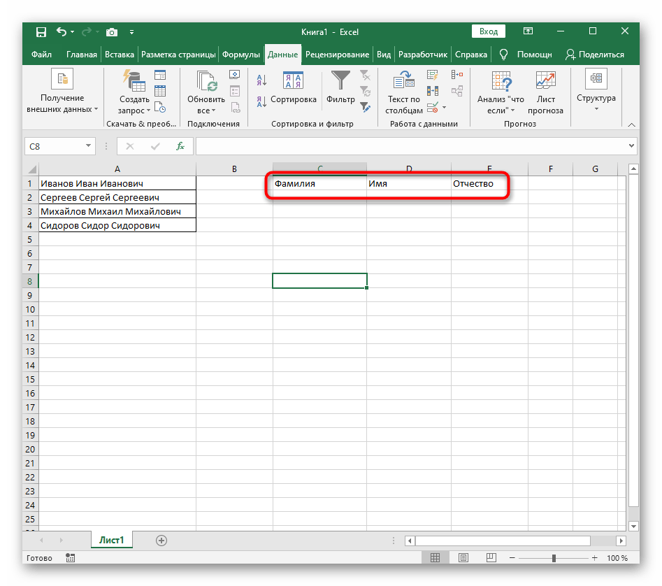
- Для удобства создадим три новые столбца с подписями, куда будем добавлять разделенный текст. Вы можете сделать так же или пропустить этот момент.
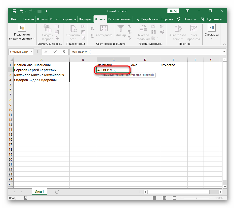
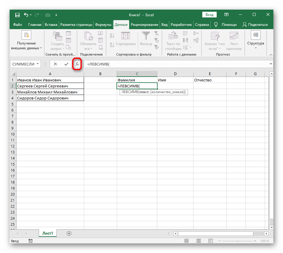
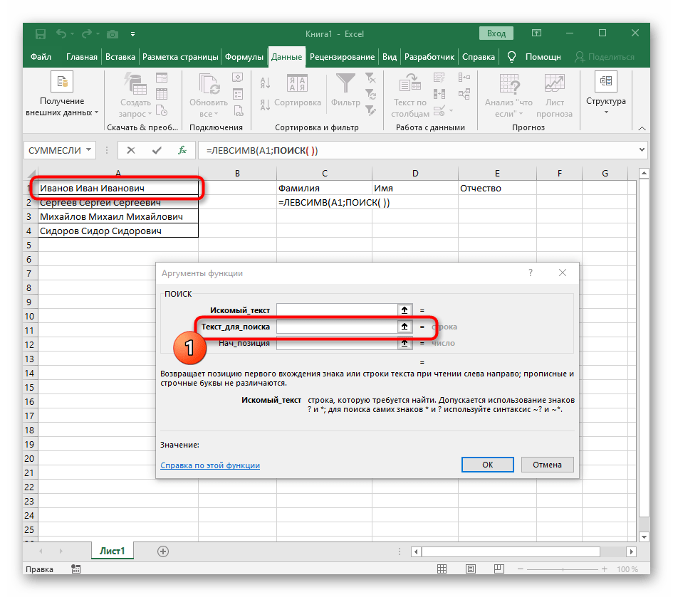
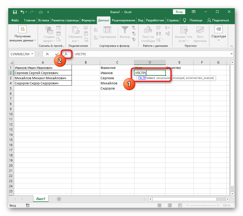
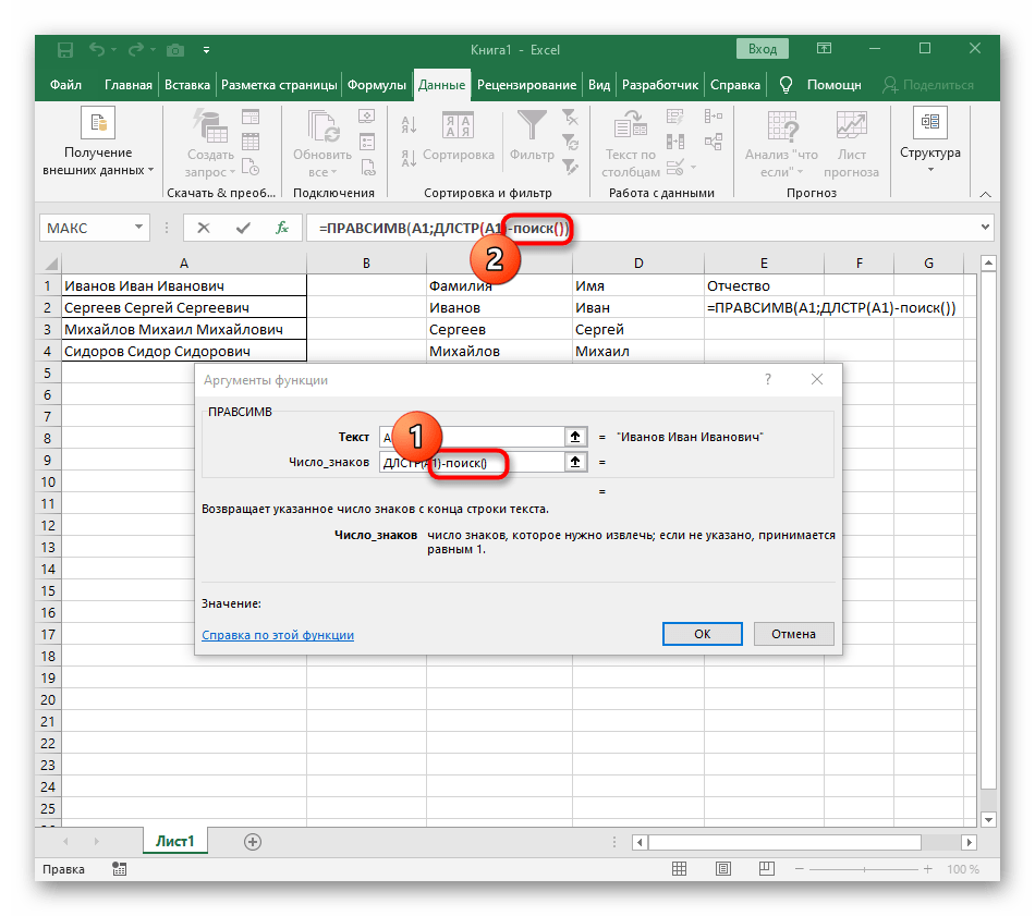
- Выберите ячейку, где хотите расположить первое слово, и запишите формулу
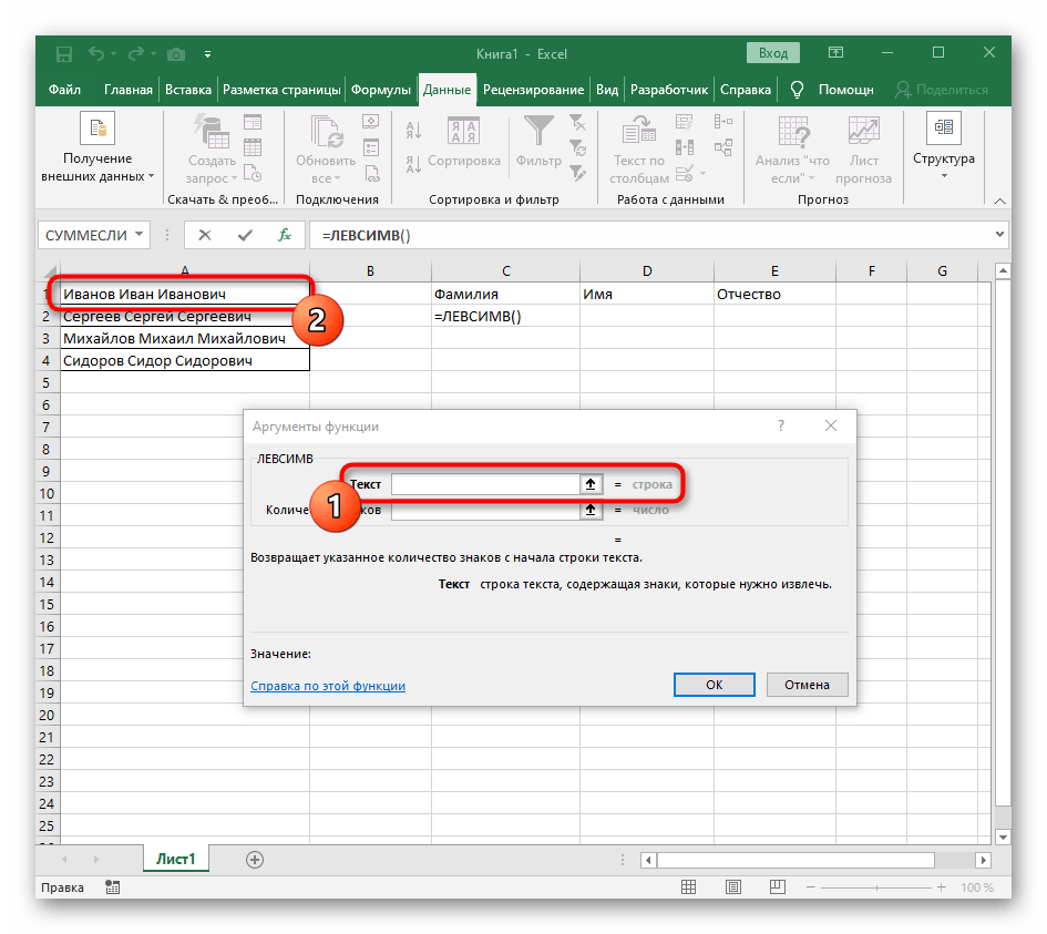
=ЛЕВСИМВ(. - После этого нажмите кнопку «Аргументы функции», перейдя тем самым в графическое окно редактирования формулы.
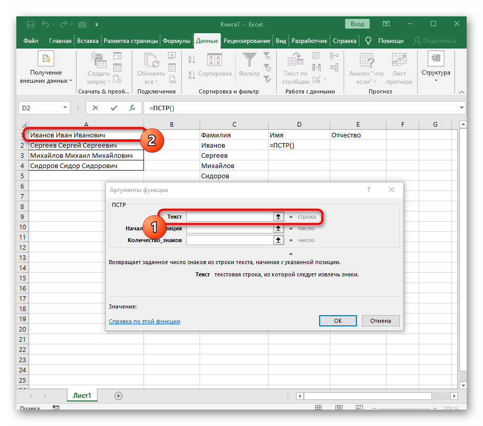
- В качестве текста аргумента указывайте ячейку с надписью, кликнув по ней левой кнопкой мыши на таблице.
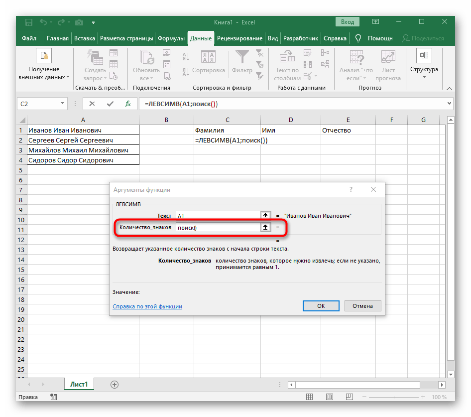
- Количество знаков до пробела или другого разделителя придется посчитать, но вручную мы это делать не будем, а воспользуемся еще одной формулой —
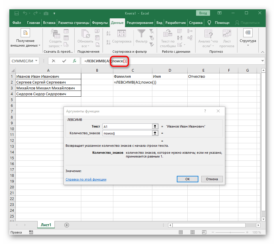
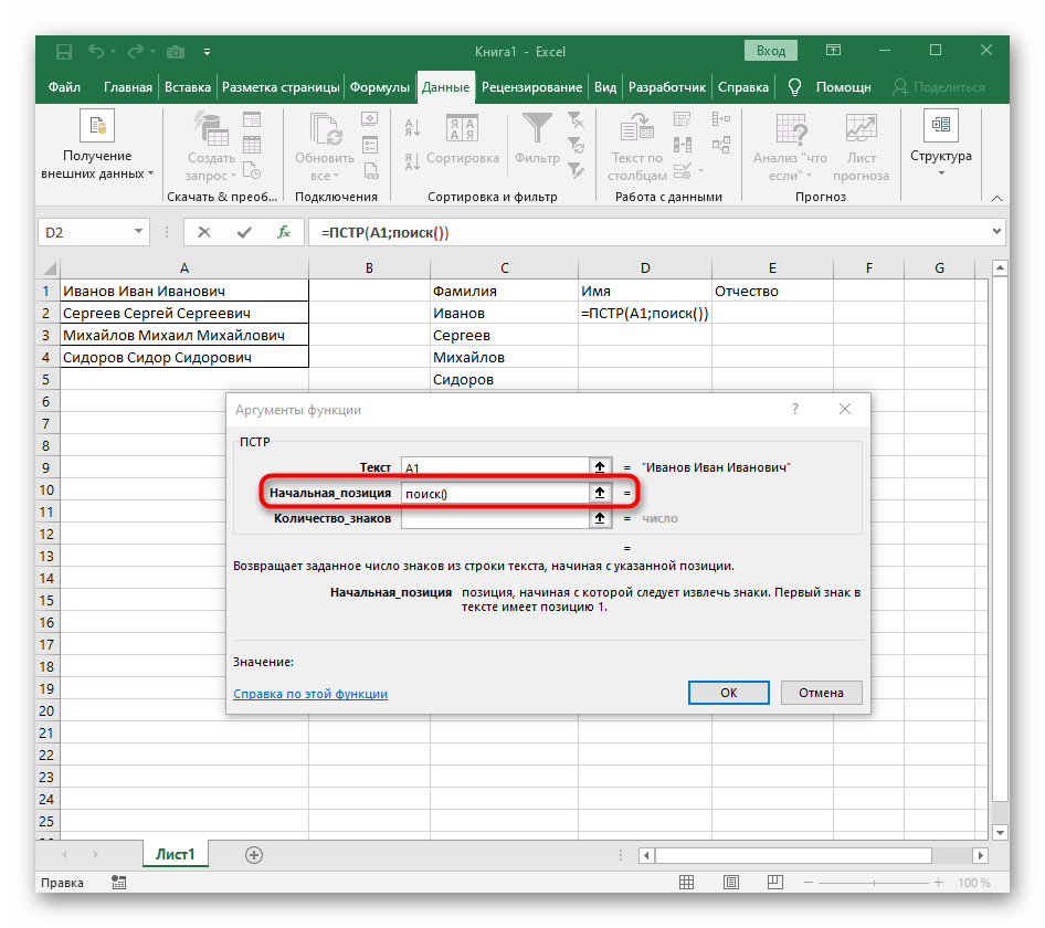
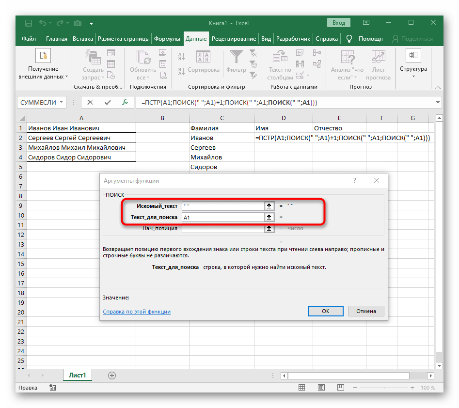
ПОИСК(). - Как только вы запишете ее в таком формате, она отобразится в тексте ячейки сверху и будет выделена жирным. Нажмите по ней для быстрого перехода к аргументам этой функции.
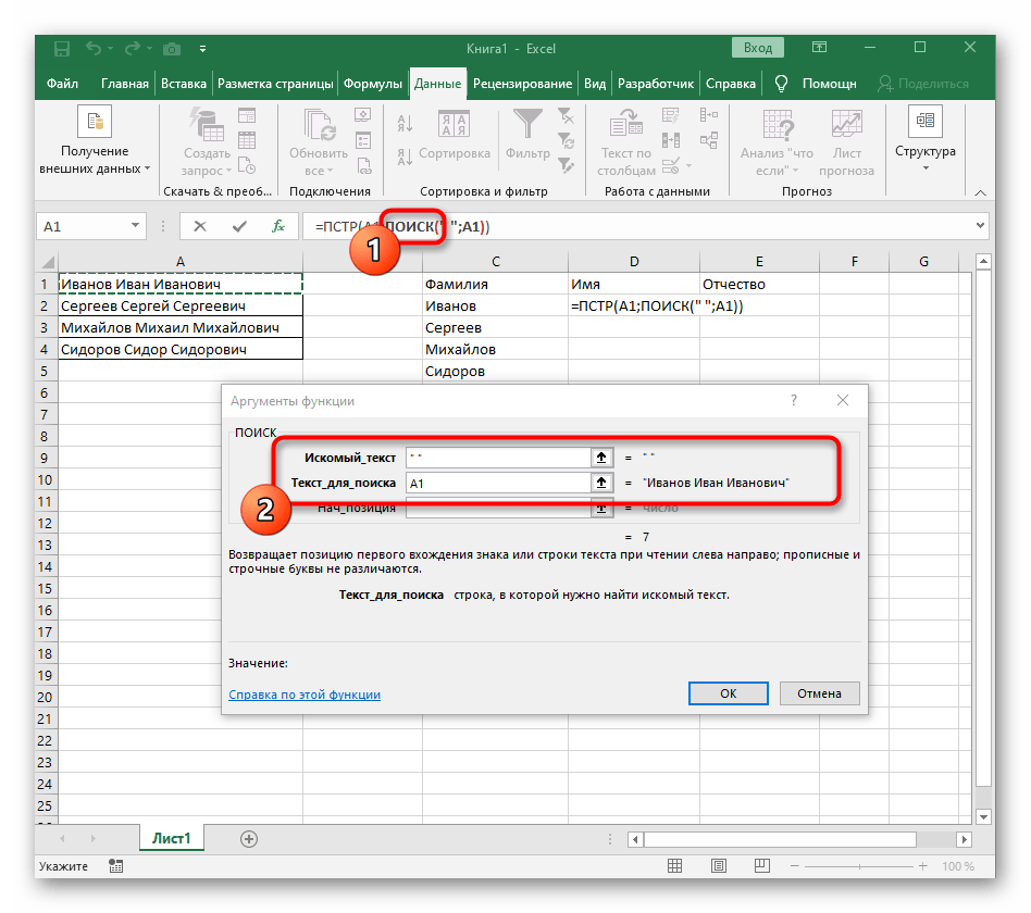
- В поле «Искомый_текст» просто поставьте пробел или используемый разделитель, поскольку он поможет понять, где заканчивается слово. В «Текст_для_поиска» укажите ту же обрабатываемую ячейку.
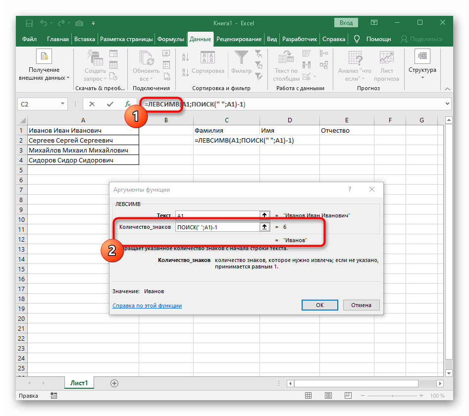
- Нажмите по первой функции, чтобы вернуться к ней, и добавьте в конце второго аргумента
-1. Это необходимо для того, чтобы формуле «ПОИСК» учитывать не искомый пробел, а символ до него. Как видно на следующем скриншоте, в результате выводится фамилия без каких-либо пробелов, а это значит, что составление формул выполнено правильно. - Закройте редактор функции и убедитесь в том, что слово корректно отображается в новой ячейке.
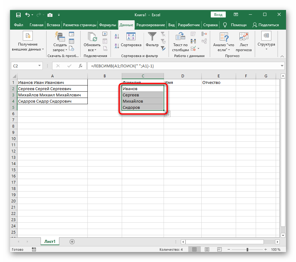
- Зажмите ячейку в правом нижнем углу и перетащите вниз на необходимое количество рядов, чтобы растянуть ее. Так подставляются значения других выражений, которые необходимо разделить, а выполнение формулы происходит автоматически.

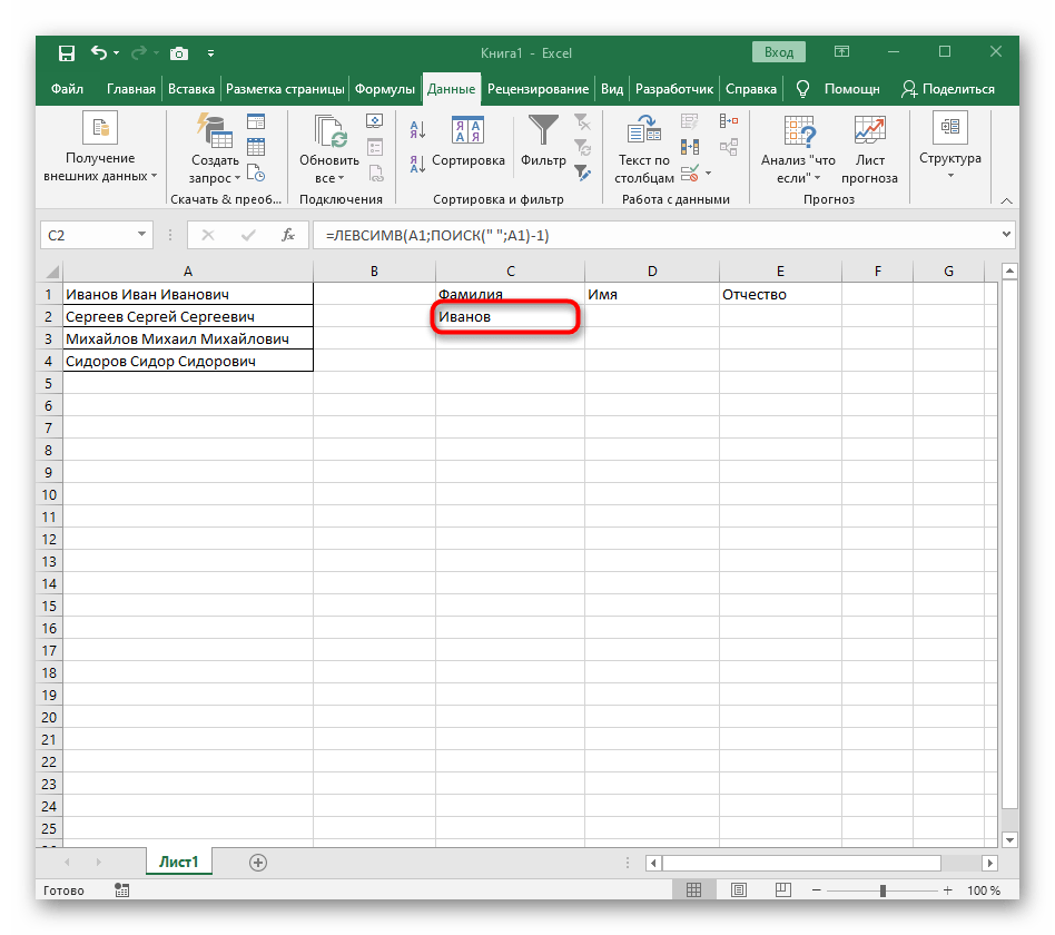
Полностью созданная формула имеет вид =ЛЕВСИМВ(A1;ПОИСК(" ";A1)-1), вы же можете создать ее по приведенной выше инструкции или вставить эту, если условия и разделитель подходят. Не забывайте заменить обрабатываемую ячейку.
Шаг 2: Разделение второго слова
Самое трудное — разделить второе слово, которым в нашем случае является имя. Связано это с тем, что оно с двух сторон окружено пробелами, поэтому придется учитывать их оба, создавая массивную формулу для правильного расчета позиции.
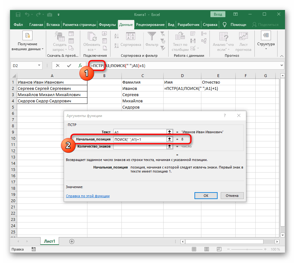
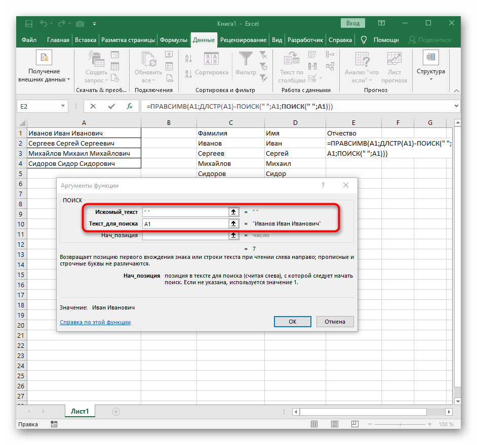
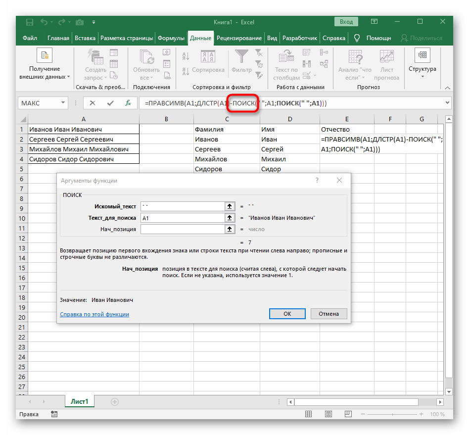
- В этом случае основной формулой станет
=ПСТР(— запишите ее в таком виде, а затем переходите к окну настройки аргументов. - Данная формула будет искать нужную строку в тексте, в качестве которого и выбираем ячейку с надписью для разделения.
- Начальную позицию строки придется определять при помощи уже знакомой вспомогательной формулы
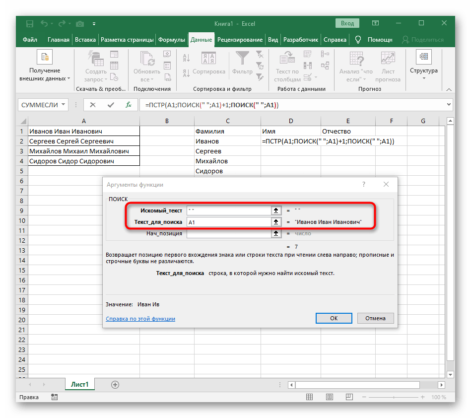
ПОИСК(). - Создав и перейдя к ней, заполните точно так же, как это было показано в предыдущем шаге. В качестве искомого текста используйте разделитель, а ячейку указывайте как текст для поиска.
- Вернитесь к предыдущей формуле, где добавьте к функции «ПОИСК»
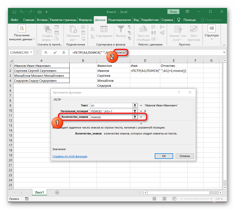
+1в конце, чтобы начинать счет со следующего символа после найденного пробела. - Сейчас формула уже может начать поиск строки с первого символа имени, но она пока еще не знает, где его закончить, поэтому в поле «Количество_знаков» снова впишите формулу
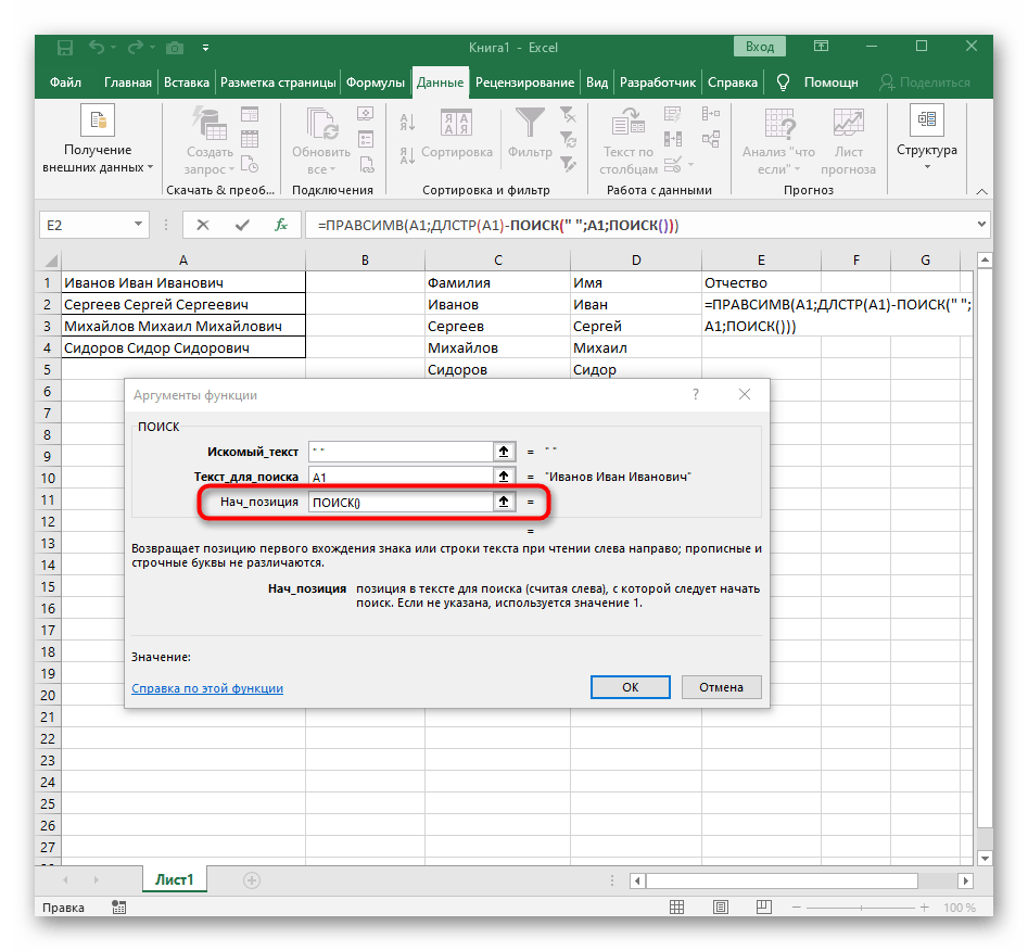
ПОИСК(). - Перейдите к ее аргументам и заполните их в уже привычном виде.
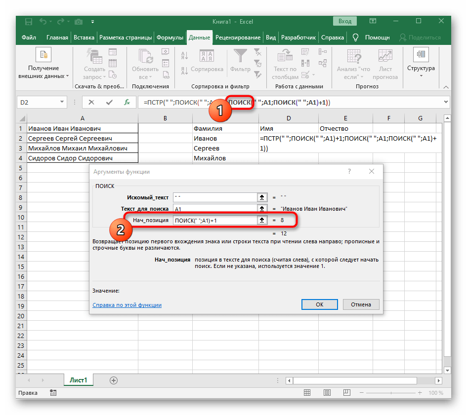
- Ранее мы не рассматривали начальную позицию этой функции, но теперь там нужно вписать тоже
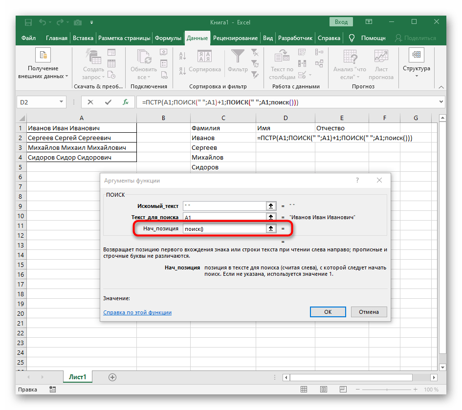
ПОИСК(), поскольку эта формула должна находить не первый пробел, а второй. - Перейдите к созданной функции и заполните ее таким же образом.
- Возвращайтесь к первому
"ПОИСКУ"и допишите в «Нач_позиция»+1в конце, ведь для поиска строки нужен не пробел, а следующий символ. - Кликните по корню
=ПСТРи поставьте курсор в конце строки «Количество_знаков». - Допишите там выражение
-ПОИСК(" ";A1)-1)для завершения расчетов пробелов. - Вернитесь к таблице, растяните формулу и удостоверьтесь в том, что слова отображаются правильно.
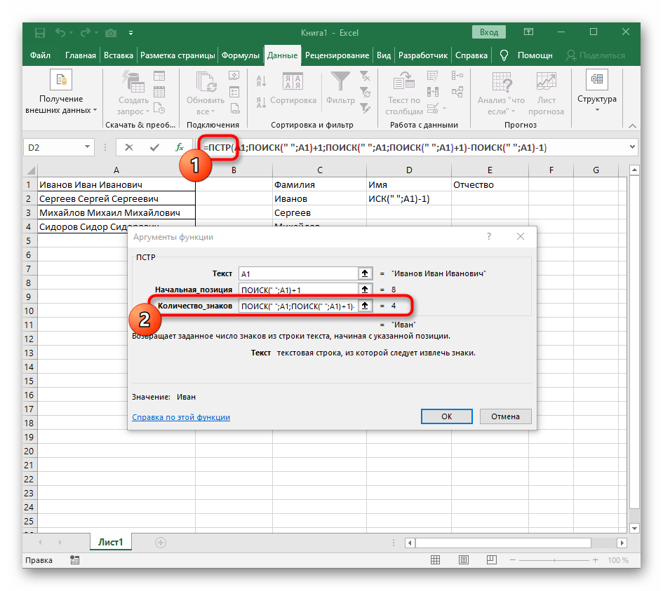
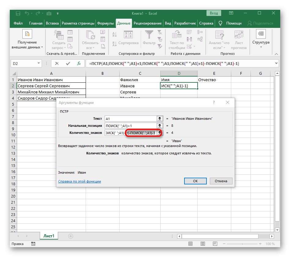
Формула получилась большая, и не все пользователи понимают, как именно она работает. Дело в том, что для поиска строки пришлось использовать сразу несколько функций, определяющих начальные и конечные позиции пробелов, а затем от них отнимался один символ, чтобы в результате эти самые пробелы не отображались. В итоге формула такая: =ПСТР(A1;ПОИСК(" ";A1)+1;ПОИСК(" ";A1;ПОИСК(" ";A1)+1)-ПОИСК(" ";A1)-1). Используйте ее в качестве примера, заменяя номер ячейки с текстом.
Шаг 3: Разделение третьего слова
Последний шаг нашей инструкции подразумевает разделение третьего слова, что выглядит примерно так же, как это происходило с первым, но общая формула немного меняется.
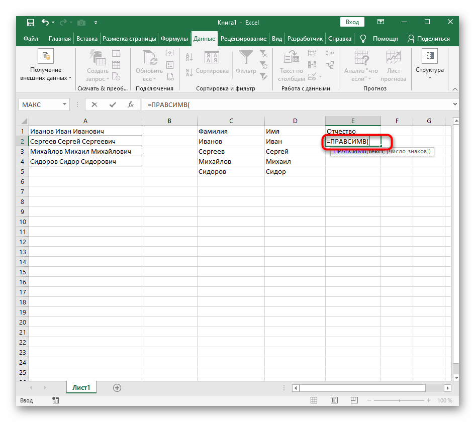
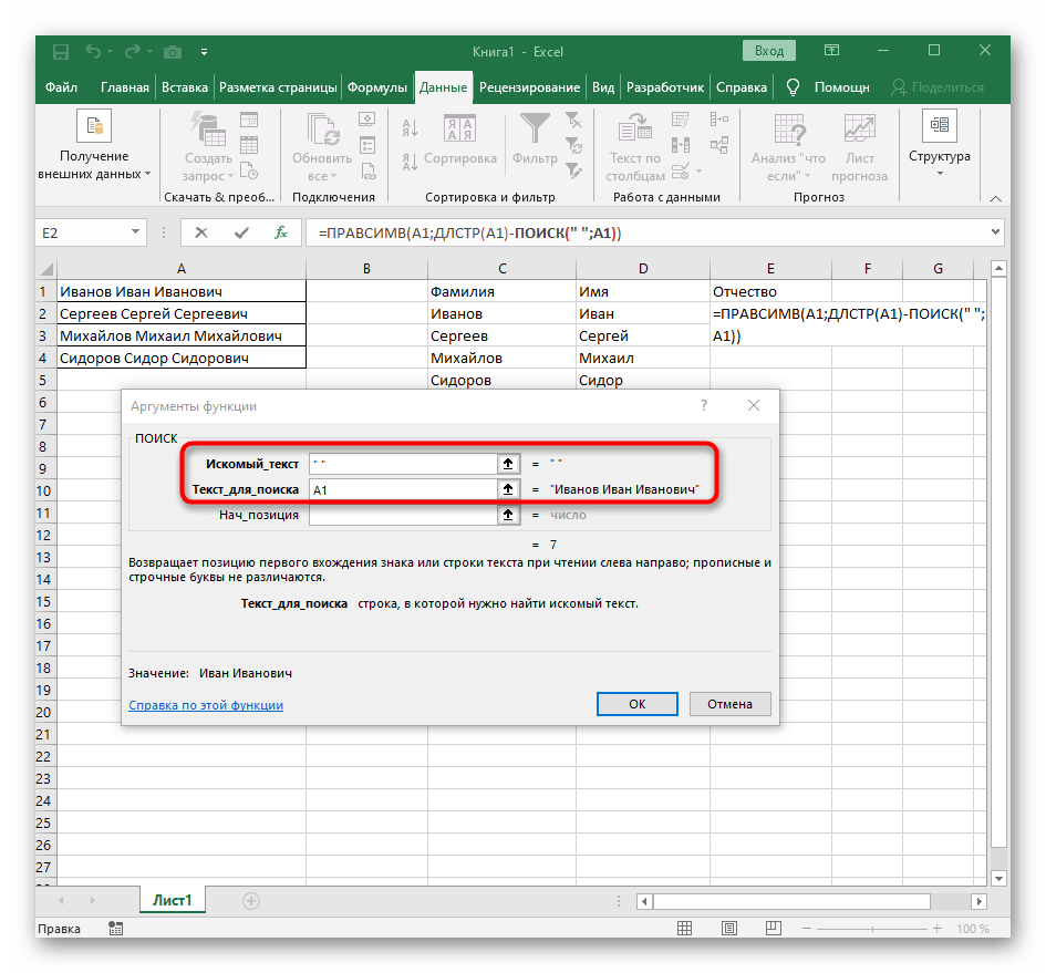
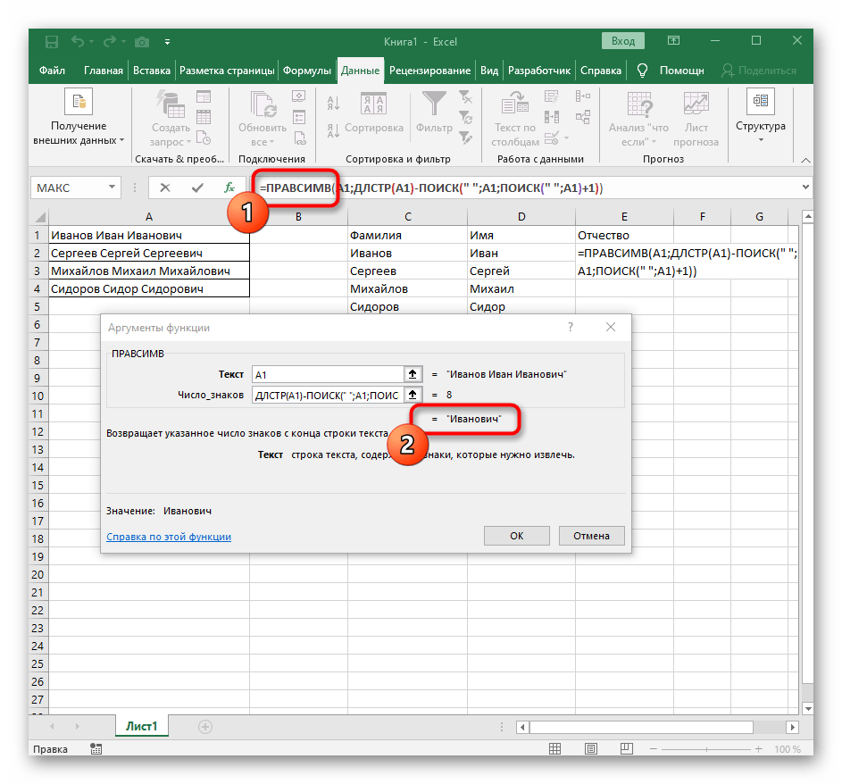
- В пустой ячейке для расположения будущего текста напишите
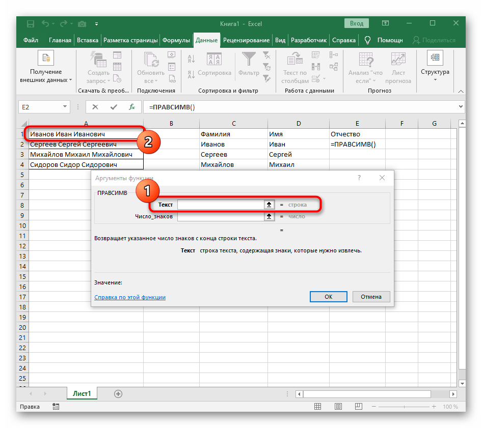
=ПРАВСИМВ(и перейдите к аргументам этой функции. - В качестве текста указывайте ячейку с надписью для разделения.
- В этот раз вспомогательная функция для поиска слова называется
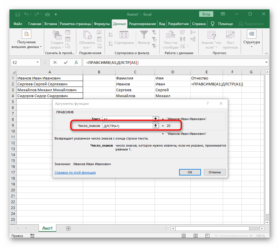
ДЛСТР(A1), где A1 — та же самая ячейка с текстом. Эта функция определяет количество знаков в тексте, а нам останется выделить только подходящие. - Для этого добавьте
-ПОИСК()и перейдите к редактированию этой формулы. - Введите уже привычную структуру для поиска первого разделителя в строке.
- Добавьте для начальной позиции еще один
ПОИСК(). - Ему укажите ту же самую структуру.
- Вернитесь к предыдущей формуле «ПОИСК».
- Прибавьте для его начальной позиции
+1. - Перейдите к корню формулы
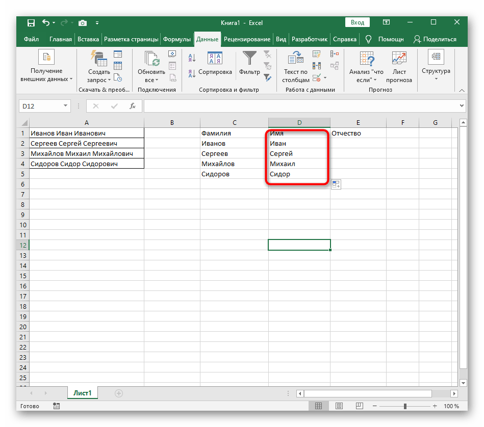
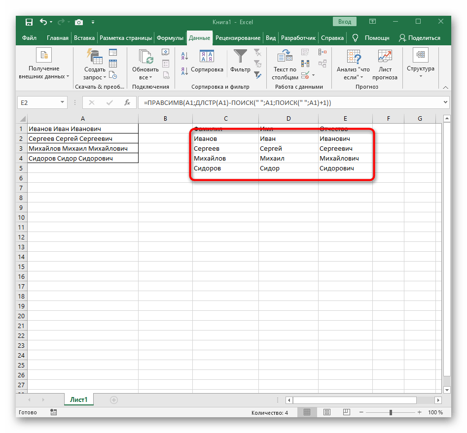
ПРАВСИМВи убедитесь в том, что результат отображается правильно, а уже потом подтверждайте внесение изменений. Полная формула в этом случае выглядит как=ПРАВСИМВ(A1;ДЛСТР(A1)-ПОИСК(" ";A1;ПОИСК(" ";A1)+1)). - В итоге на следующем скриншоте вы видите, что все три слова разделены правильно и находятся в своих столбцах. Для этого пришлось использовать самые разные формулы и вспомогательные функции, но это позволяет динамически расширять таблицу и не беспокоиться о том, что каждый раз придется разделять текст заново. По необходимости просто расширяйте формулу путем ее перемещения вниз, чтобы следующие ячейки затрагивались автоматически.

Еще статьи по данной теме:
Помогла ли Вам статья?
When data is imported into Excel it can be in many formats depending on the source application that has provided it.
For example, it could contain names and addresses of customers or employees, but this all ends up as a continuous text string in one column of the worksheet, instead of being separated out into individual columns e.g. name, street, city.
You can split the data by using a common delimiter character. A delimiter character is usually a comma, tab, space, or semi-colon. This character separates each chunk of data within the text string.
A big advantage of using a delimiter character is that it does not rely on fixed widths within the text. The delimiter indicates exactly where to split the text.
You may need to split the data because you may want to sort the data using a certain part of the address or to be able to filter on a particular component. If the data is used in a pivot table, you may need to have the name and address as different fields within it.
This article shows you eight ways to split the text into the component parts required by using a delimiter character to indicate the split points.
Sample Data
The above sample data will be used in all the following examples. Download the example file to get the sample data plus the various solutions for extracting data based on delimiters.
Excel Functions to Split Text
There are several Excel functions that can be used to split and manipulate text within a cell.
LEFT Function
The LEFT function returns the number of characters from the left of the text.
Syntax
= LEFT ( Text, [Number] )- Text – This is the text string that you wish to extract from. It can also be a valid cell reference within a workbook.
- Number [Optional] – This is the number of characters that you wish to extract from the text string. The value must be greater than or equal to zero. If the value is greater than the length of the text string, then all characters will be returned. If the value is omitted, then the value is assumed to be one.
RIGHT Function
The RIGHT function returns the number of characters from the right of the text.
Syntax
= RIGHT ( Text, [Number] )The parameters work in the same way as for the LEFT function described above.
FIND Function
The FIND function returns the position of specified text within a text string. This can be used for locating a delimiter character. Note that the search is case-sensitive.
Syntax
= FIND (SubText, Text, [Start])- SubText – This is a text string that you want to search for.
- Text – This is the text string which is to be searched.
- Start [Optional] – The starting position for the search.
LEN Function
The LEN function will give the length by number of characters of a text string.
Syntax
= LEN ( Text )- Text – This is the text string of which you want to determine the character count.
Extracting Data with the LEFT, RIGHT, FIND and LEN Functions
Using the first row (B3) of the sample data, these functions can be combined to split a text string into sections using a delimiter character.
= FIND ( ",", B3 )You use the FIND function to get the position of the first delimiter character. This will return the value 18.
= LEFT ( B3, FIND( ",", B3 ) - 1 )You can then use the LEFT function to extract the first component of the text string.
Note that FIND gets the position of the first delimiter, but you need to subtract 1 from it so as to not include the delimiter character.
This will return Tabbie O’Hallagan.
= RIGHT ( B3, LEN ( B3 ) - FIND ( ",", B3 ) )It is more complicated to get the next components of the text string. You need to remove the first component from the text by using the above formula.
This formula takes the length of the original text, finds the first delimiter position, which then calculates how many characters are left in the text string after that delimiter.
The RIGHT function then truncates off all the characters up to and including that first delimiter so that the text string gets shorter and shorter as each delimiter character is found.
This will return 056 Dennis Park, Greda, Croatia, 44273
You can now use FIND to locate the next delimiter and the LEFT function to extract the next component, using the same methodology as above.
Repeat for all delimiters, and this will split the text string into component parts.
FILTERXML Function as a Dynamic Array
If you’re using Excel for Microsoft 365, then you can use the FILTERXML function to split text with output as a dynamic array.
You can split a text string by turning it into an XML string by changing the delimiter characters to XML tags. This way you can use the FILTERXML function to extract data.
XML tags are user defined, but in this example, s will represent a sub-node and t will represent the main node.
= "<t><s>" & SUBSTITUTE ( B2, ",", "</s><s>" ) & "</s></t>"Use the above formula to insert the XML tags into your text string.
<t><s>Name</s><s>Street</s><s>City</s><s>Country</s><s>Post Code</s></t>This will return the above formula in the example.
Note that each of the nodes defined is followed by a closing node with a backslash. These XML tags define the start and finish of each section of the text, and effectively act in the same way as delimiters.
=TRANSPOSE(
    FILTERXML(
        "<t><s>" &
        SUBSTITUTE(
            B3,
            ",",
            "</s><s>"
        ) & "</s></t>",
        "//s"
    )
)
The above formula will insert the XML tags into the original string and then use these to split out the items into an array.
As seen above, the array will spill each item into a separate cell. Using the TRANSPOSE function causes the array to spill horizontally instead of vertically.
FILTERXML Function to Split Text
If your version of Excel doesn’t have dynamic arrays, then you can still use the FILTERXML function to extract individual items.
= FILTERXML (
    "<t><s>" &
    SUBSTITUTE (
        B3,
        ",",
        "</s><s>"
    ) & "</s></t>",
    "//s"
)
You can now break the string into sections using the above FILTERXML formula.
This will return the first section Tabbie O’Hallagan.
= FILTERXML (
    "<t><s>" &
    SUBSTITUTE (
        B3,
        ",",
        "</s><s>"
    ) & "</s></t>",
    "//s[2]"
)
To return the next section, use the above formula.
This will return the second section of the text string 056 Dennis Park.
You can use this same pattern to return any part of the sample text, just change the [2] found in the formula accordingly.
Flash Fill to Split Text
Flash Fill allows you to put in an example of how you want your data split.
You can check out this guide on using flash fill to clean your data for more details.
You then select the first cell of where you want your data to split and click on Flash Fill. Excel will populate the remaining rows from your example.
Using the sample data, enter Name into cell C2, then Tabbie O’Hallagan into cell C3.
Flash fill should automatically fill in the remaining data names from the sample data. If it doesn’t, you can select cell C4, and click on the Flash Fill icon in the Data Tools group of the Data tab of the Excel ribbon.
Similarly, you can add Street into cell D2, City into cell E2, Country into cell F2, and Post Code into cell G2.
Select the subsequent cells (D2 to G2) individually, and click on the Flash Fill icon. The rest of the text components will be populated into these columns.
Text to Columns Command to Split Text
This Excel functionality can be used to split text in a cell into sections based on a delimiter character.
- Select the entire sample data range (B2:B12).
- Click on the Data tab in the Excel ribbon.
- Click on the Text to Columns icon in the Data Tools group of the Excel ribbon and a wizard will appear to help you set up how the text will be split.
- Select Delimited on the option buttons.
- Press the Next button.
- Select Comma as the delimiter, and uncheck any other delimiters.
- Press the Next button.
- The Data Preview window will display how your data will be split. Choose a location to place the output.
- Click on Finish button.
Your data will now be displayed in columns on your worksheet.
Convert the Data into a CSV File
This will only work with commas as delimiters, since a CSV (comma separated value) file depends on commas to separate the values.
Open Notepad and copy and paste the sample data into it. You can open Notepad by typing Notepad into the search box at the left of the Windows task bar or locate it in the application list.
Once you have copied the data into Notepad, save it off by using File ➜ Save As from the menu. Enter a filename with a .csv suffix e.g. Split Data.csv.
You can then open this file in Excel. Select the csv file in the browser file type drop down and click OK. Your data will automatically appear with each component in separate columns.
VBA to Split Text
VBA is the programming language that sits behind Excel and allows you to write your own code to manipulate data, or to even create your own functions.
To access the Visual Basic Editor (VBE), you use Alt + F11.
Sub SplitText()

Dim MyArray() As String, Count As Long, i As Variant

For n = 2 To 12
	MyArray = Split(Cells(n, 2), ",")
	Count = 3
	For Each i In MyArray
		Cells(n, Count) = i
		Count = Count + 1
	Next i
Next n

End Sub
Click on Insert in the menu bar, and click on Module. A new pane will appear for the module. Paste in the above code.
This code creates a single dimensional array called MyArray. It then iterates through the sample data (rows 2 to 12) and uses the VBA Split function to populate MyArray.
The split function uses a comma delimiter, so that each section of the text becomes an element of the array.
A counter variable is set to 3 which represents column C, which will be the first column for the split data to be displayed.
The code then iterates through each element in the array and populates each cell with the element. Cell references are based on n for the row, and Count for the column.
The variable Count is incremented in each loop so that the data fills across the row, and then downwards.
Power Query to Split Text
Power Query in Excel allows a column to be manipulated into sections using a delimiter character.
Related posts:
- Introduction to power query
- Power query tips and tricks
- Introduction to power query M code
The first thing to do is to define your data source, which is the sample data that you entered into you Excel worksheet.
Click on the Data tab in the Excel ribbon, and then click on Get Data in the Get & Transform Data group of the ribbon.
Click on From File in the first drop down, and then click on From Workbook in the second drop down.
This will display a file browser. Locate your sample data file (the file that you have open) and click on OK.
A navigation pop-up will be displayed showing all the worksheets within your workbook. Click on the worksheet which has the sample data and this will show a preview of the data.
Expand the tree of data in the left-hand pane to show the preview of the existing data.
Click on Transform Data and this will display the Power Query Editor.
Make sure that the single column with the data in it is highlighted. Click on the Split Column icon in the Transform group of the ribbon. Click on By Delimiter in the drop down that appears.
This will display a pop-up window which allows you to select your delimiter. The default is a comma.
Click OK and the data will be transformed into separate columns.
Click on Close and Load in the Close group of the ribbon, and a new worksheet will be added to your workbook with a table of the data in the new format.
Power Pivot Calculated Column to Split Text
You can use Power Pivot to split the text by using calculated columns.
Click on the Power Pivot tab in the Excel ribbon and then click on the Add to Data Model icon in the Tables group.
Your data will be automatically detected and a pop-up will show the location. If this is not the correct location, then it can be re-set here.
Leave the My table has headers check box un-ticked in the pop-up, as we want to split the header as well.
Click on OK and a preview screen will be displayed.
Right-click on the header for your data column (Column1) and click on Insert Column in the pop-up menu. This will insert a calculated column where a formula can be entered.
= LEFT ( [Column1], FIND ( ",", [Column1] ) - 1 )In the formula bar, insert the above formula.
This works in a similar way to the functions described in method 1 of this article.
This formula will provide the Name component within the text string.
Insert another calculated column using the same methodology as the first calculated column.
= LEFT (
    RIGHT ( [Column1], LEN ( [column1] ) - LEN ( [Calculated Column 1] ) - 1 ),
    FIND (
        ",",
        RIGHT ( [Column1], LEN ( [column1] ) - LEN ( [Calculated Column 1] ) - 1 )
    ) - 1
)
Insert the above formula into the formula bar.
This is a complicated formula, and you may wish to break it into sections using several calculated columns.
This will provide the Street component in the text string.
You can continue modifying the formula to create calculated columns for all the other components of the text string.
The problem with a pivot table is that it needs a numeric value as well as text values. As the sample data is text only, a numeric value needs to be added.
Click on the first cell in the Add Column column and enter the formula =1 in the formula bar.
This will add the value of 1 all the way down that column. Click on the Pivot Table icon in the Home tab of the ribbon.
Click on Pivot Table in the pop-up menu. Specify the location of your pivot table in the first pop-up window and click OK. If the Pivot Table Fields pane does not automatically display, right click on the pivot table skeleton and select Show Field List.
Click on the Calculated Columns in the Field List and place these in the Rows window.
our pivot table will now show the individual components of the text string.
Conclusions
Dealing with comma or other delimiter separated data can be a big pain if you don’t know how to extract each item into its own cell.
Thankfully, Excel has quite a few options that will help with this common task.
Which one do you prefer to use?
About the Author
John is a Microsoft MVP and qualified actuary with over 15 years of experience. He has worked in a variety of industries, including insurance, ad tech, and most recently Power Platform consulting. He is a keen problem solver and has a passion for using technology to make businesses more efficient.
Skip to content
В руководстве объясняется, как разделить ячейки в Excel с помощью формул и стандартных инструментов. Вы узнаете, как разделить текст запятой, пробелом или любым другим разделителем, а также как разбить строки на текст и числа.
Разделение текста из одной ячейки на несколько — это задача, с которой время от времени сталкиваются все пользователи Excel. В одной из наших предыдущих статей мы обсуждали, как разделить ячейки в Excel с помощью функции «Текст по столбцам» и «Мгновенное заполнение». Сегодня мы подробно рассмотрим, как можно разделить текст по ячейкам с помощью формул.
Чтобы разбить текст в Excel, вы обычно используете функции ЛЕВСИМВ (LEFT), ПРАВСИМВ (RIGHT) или ПСТР (MID) в сочетании с НАЙТИ (FIND) или ПОИСК (SEARCH). На первый взгляд, некоторые рассмотренные ниже приёмы могут показаться сложными. Но на самом деле логика довольно проста, и следующие примеры помогут вам разобраться.
Для преобразования текста в ячейках в Excel ключевым моментом является определение положения разделителя в нем. Что может быть таким разделителем? Это запятая, точка с запятой, наклонная черта, двоеточие, тире, восклицательный знак и т.п. И, как мы далее увидим, даже целое слово.
- Как распределить ФИО по столбцам
- Как использовать разделители в тексте
- Разделяем текст по переносам строки
- Как разделить длинный текст на множество столбцов
- Как разбить «текст + число» по разным ячейкам
- Как разбить ячейку вида «число + текст»
- Разделение ячейки по маске (шаблону)
- Использование инструмента Split Text
В зависимости от вашей задачи эту проблему можно решить с помощью функции ПОИСК (без учета регистра букв) или НАЙТИ (с учетом регистра).
Как только вы определите позицию разделителя, используйте функцию ЛЕВСИМВ, ПРАВСИМВ и ПСТР, чтобы извлечь соответствующую часть содержимого.
Для лучшего понимания пошагово рассмотрим несколько примеров.
Делим текст вида ФИО по столбцам.
Если выяснение загадочных поворотов формул Excel — не ваше любимое занятие, вам может понравиться визуальный метод разделения ячеек, который демонстрируется ниже.
В столбце A нашей таблицы записаны Фамилии, имена и отчества сотрудников. Необходимо разделить их на 3 столбца.
Можно сделать это при помощи инструмента «Текст по столбцам». Об этом методе мы достаточно подробно рассказывали, когда рассматривали, как можно разделить ячейку по столбцам.
Кратко напомним:
На ленте «Данные» выбираем «Текст по столбцам» — с разделителями.

Далее в качестве разделителя выбираем пробел.
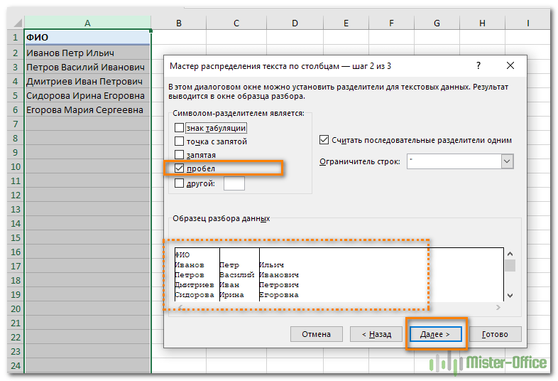
Обращаем внимание на то, как разделены наши данные в окне образца.
В следующем окне определяем формат данных. По умолчанию там будет «Общий». Он нас вполне устраивает, поэтому оставляем как есть. Выбираем левую верхнюю ячейку диапазона, в который будет помещен наш разделенный текст. Если нужно оставить в неприкосновенности исходные данные, лучше выбрать B1, к примеру.
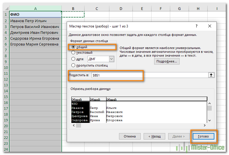
В итоге имеем следующую картину:

При желании можно дать заголовки новым столбцам B,C,D.
А теперь давайте тот же результат получим при помощи формул.
Для многих это удобнее. В том числе и по той причине, что если в таблице появятся новые данные, которые нужно разделить, то нет необходимости повторять всю процедуру с начала, а просто нужно скопировать уже имеющиеся формулы.
Итак, чтобы выделить из нашего ФИО фамилию, будем использовать выражение
=ЛЕВСИМВ(A2; ПОИСК(» «;A2;1)-1)
В качестве разделителя мы используем пробел. Функция ПОИСК указывает нам, в какой позиции находится первый пробел. А затем именно это количество букв (за минусом 1, чтобы не извлекать сам пробел) мы «отрезаем» слева от нашего ФИО при помощи ЛЕВСИМВ.
Далее будет чуть сложнее.
Нужно извлечь второе слово, то есть имя. Чтобы вырезать кусочек из середины, используем функцию ПСТР.
=ПСТР(A2; ПОИСК(» «;A2) + 1; ПОИСК(» «;A2;ПОИСК(» «;A2)+1) — ПОИСК(» «;A2) — 1)
Как вы, наверное, знаете, функция Excel ПСТР имеет следующий синтаксис:
ПСТР (текст; начальная_позиция; количество_знаков)
Текст извлекается из ячейки A2, а два других аргумента вычисляются с использованием 4 различных функций ПОИСК:
- Начальная позиция — это позиция первого пробела плюс 1:
ПОИСК(» «;A2) + 1
- Количество знаков для извлечения: разница между положением 2- го и 1- го пробелов, минус 1:
ПОИСК(» «;A2;ПОИСК(» «;A2)+1) — ПОИСК(» «;A2) – 1
В итоге имя у нас теперь находится в C.
Осталось отчество. Для него используем выражение:
=ПРАВСИМВ(A2;ДЛСТР(A2) — ПОИСК(» «; A2; ПОИСК(» «; A2) + 1))
В этой формуле функция ДЛСТР (LEN) возвращает общую длину строки, из которой вы вычитаете позицию 2- го пробела. Получаем количество символов после 2- го пробела, и функция ПРАВСИМВ их и извлекает.
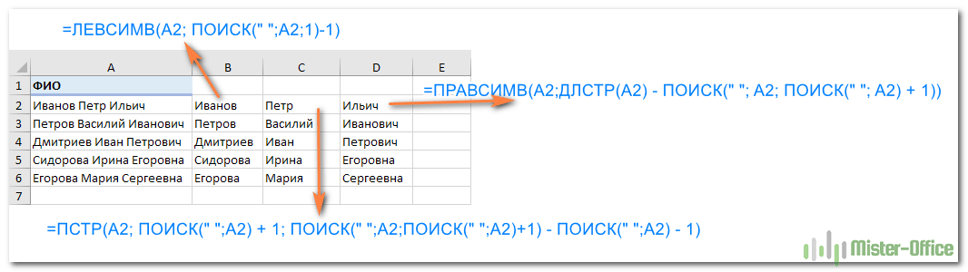
Вот результат нашей работы по разделению фамилии, имени и отчества из одной по отдельным ячейкам.
Распределение текста с разделителями на 3 столбца.
Предположим, у вас есть список одежды вида Наименование-Цвет-Размер, и вы хотите разделить его на 3 отдельных части. Здесь разделитель слов – дефис. С ним и будем работать.
- Чтобы извлечь Наименование товара (все символы до 1-го дефиса), вставьте следующее выражение в B2, а затем скопируйте его вниз по столбцу:
=ЛЕВСИМВ(A2; ПОИСК(«-«;A2;1)-1)
Здесь функция мы сначала определяем позицию первого дефиса («-«) в строке, а ЛЕВСИМВ извлекает все нужные символы начиная с этой позиции. Вы вычитаете 1 из позиции дефиса, потому что вы не хотите извлекать сам дефис.
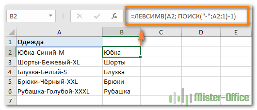
- Чтобы извлечь цвет (это все буквы между 1-м и 2-м дефисами), запишите в C2, а затем скопируйте ниже:
=ПСТР(A2; ПОИСК(«-«;A2) + 1; ПОИСК(«-«;A2;ПОИСК(«-«;A2)+1) — ПОИСК(«-«;A2) — 1)
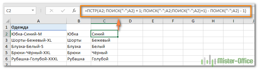
Логику работы ПСТР мы рассмотрели чуть выше.
- Чтобы извлечь размер (все символы после 3-го дефиса), введите следующее выражение в D2:
=ПРАВСИМВ(A2;ДЛСТР(A2) — ПОИСК(«-«; A2; ПОИСК(«-«; A2) + 1))

Аналогичным образом вы можете в Excel разделить содержимое ячейки в разные ячейки любым другим разделителем. Все, что вам нужно сделать, это заменить «-» на требуемый символ, например пробел (« »), косую черту («/»), двоеточие («:»), точку с запятой («;») и т. д.
Примечание. В приведенных выше формулах +1 и -1 соответствуют количеству знаков в разделителе. В нашем примере это дефис (то есть, 1 знак). Если ваш разделитель состоит из двух знаков, например, запятой и пробела, тогда укажите только запятую («,») в ваших выражениях и используйте +2 и -2 вместо +1 и -1.
Как разбить текст по переносам строки.
Чтобы разделить слова в ячейке по переносам строки, используйте подходы, аналогичные тем, которые были продемонстрированы в предыдущем примере. Единственное отличие состоит в том, что вам понадобится функция СИМВОЛ (CHAR) для передачи символа разрыва строки, поскольку вы не можете ввести его непосредственно в формулу с клавиатуры.
Предположим, ячейки, которые вы хотите разделить, выглядят примерно так:

Напомню, что перенести таким вот образом текст внутри ячейки можно при помощи комбинации клавиш ALT + ENTER.
Возьмите инструкции из предыдущего примера и замените дефис («-») на СИМВОЛ(10), где 10 — это код ASCII для перевода строки.
Чтобы извлечь наименование товара:
=ЛЕВСИМВ(A2; ПОИСК(СИМВОЛ(10);A2;1)-1)
Цвет:
=ПСТР(A2; ПОИСК(СИМВОЛ(10);A2) + 1; ПОИСК(СИМВОЛ(10);A2; ПОИСК(СИМВОЛ(10);A2)+1) — ПОИСК(СИМВОЛ(10);A2) — 1)
Размер:
=ПРАВСИМВ(A2;ДЛСТР(A2) — ПОИСК(СИМВОЛ(10); A2; ПОИСК(СИМВОЛ(10); A2) + 1))
Результат вы видите на скриншоте выше.
Таким же образом можно работать и с любым другим символом-разделителем. Достаточно знать его код.
Как распределить текст с разделителями на множество столбцов.
Изучив представленные выше примеры, у многих из вас, думаю, возник вопрос: «А что, если у меня не 3 слова, а больше? Если нужно разбить текст в ячейке на 5 столбцов?»
Если действовать методами, описанными выше, то формулы будут просто мега-сложными. Вероятность ошибки при их использовании очень велика. Поэтому мы применим другой метод.
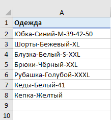
Имеем список наименований одежды с различными признаками, перечисленными через дефис. Как видите, таких признаков у нас может быть от 2 до 6. Делим текст в наших ячейках на 6 столбцов так, чтобы лишние столбцы в отдельных строках просто остались пустыми.
Для первого слова (наименования одежды) используем:
=ЛЕВСИМВ(A2; ПОИСК(«-«;A2;1)-1)
Как видите, это ничем не отличается от того, что мы рассматривали ранее. Ищем позицию первого дефиса и отделяем нужное количество символов.
Для второго столбца и далее понадобится более сложное выражение:
=ЕСЛИОШИБКА(ЛЕВСИМВ(ПОДСТАВИТЬ($A2&»-«; ОБЪЕДИНИТЬ(«-«;ИСТИНА;$B2:B2)&»-«;»»;1); ПОИСК(«-«;ПОДСТАВИТЬ($A2&»-«;ОБЪЕДИНИТЬ(«-«;ИСТИНА;$B2:B2)&»-«;»»;1);1)-1);»»)
Замысел здесь состоит в том, что при помощи функции ПОДСТАВИТЬ мы удаляем из исходного содержимого наименование, которое уже ранее извлекли (то есть, «Юбка»). Вместо него подставляем пустое значение «» и в результате имеем «Синий-M-39-42-50». В нём мы снова ищем позицию первого дефиса, как это делали ранее. И при помощи ЛЕВСИМВ вновь выделяем первое слово (то есть, «Синий»).
А далее можно просто «протянуть» формулу из C2 по строке, то есть скопировать ее в остальные ячейки. В результате в D2 получим
=ЕСЛИОШИБКА(ЛЕВСИМВ(ПОДСТАВИТЬ($A2&»-«; ОБЪЕДИНИТЬ(«-«;ИСТИНА;$B2:C2)&»-«;»»;1); ПОИСК(«-«;ПОДСТАВИТЬ($A2&»-«;ОБЪЕДИНИТЬ(«-«;ИСТИНА;$B2:C2)&»-«;»»;1);1)-1);»»)
Обратите внимание, жирным шрифтом выделены произошедшие при копировании изменения. То есть, теперь из исходного текста мы удаляем все, что было уже ранее найдено и извлечено – содержимое B2 и C2. И вновь в получившейся фразе берём первое слово — до дефиса.
Если же брать больше нечего, то функция ЕСЛИОШИБКА обработает это событие и вставит в виде результата пустое значение «».
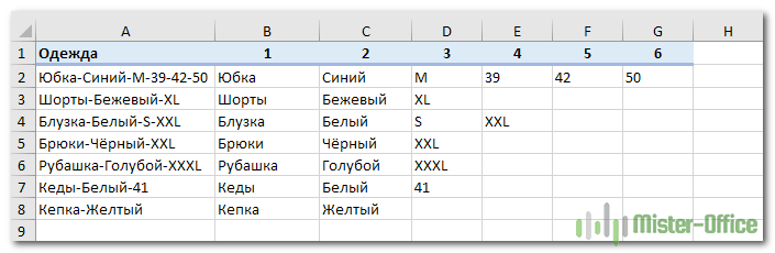
Скопируйте формулы по строкам и столбцам, на сколько это необходимо. Результат вы видите на скриншоте.
Таким способом можно разделить текст в ячейке на сколько угодно столбцов. Главное, чтобы использовались одинаковые разделители.
Как разделить ячейку вида ‘текст + число’.
Начнем с того, что не существует универсального решения, которое работало бы для всех буквенно-цифровых выражений. Выбор зависит от конкретного шаблона, по которому вы хотите разбить ячейку. Ниже вы найдете формулы для двух наиболее распространенных сценариев.
Предположим, у вас есть столбец смешанного содержания, где число всегда следует за текстом. Естественно, такая конструкция рассматривается Excel как символьная. Вы хотите поделить их так, чтобы текст и числа отображались в отдельных ячейках.
Результат может быть достигнут двумя разными способами.
Метод 1. Подсчитайте цифры и извлеките это количество символов
Самый простой способ разбить выражение, в котором число идет после текста:
Чтобы извлечь числа, вы ищите в строке все возможные числа от 0 до 9, получаете общее их количество и отсекаете такое же количество символов от конца строки.
Если мы работаем с ячейкой A2:
=ПРАВСИМВ(A2;СУММ(ДЛСТР(A2) — ДЛСТР(ПОДСТАВИТЬ(A2; {«0″;»1″;»2″;»3″;»4″;»5″;»6″;»7″;»8″;»9″};»»))))
Чтобы извлечь буквы, вы вычисляете, сколько их у нас имеется. Для этого вычитаем количество извлеченных цифр (C2) из общей длины исходной ячейки A2. После этого при помощи ЛЕВСИМВ отрезаем это количество символов от начала ячейки.
=ЛЕВСИМВ(A2;ДЛСТР(A2)-ДЛСТР(C2))
здесь A2 – исходная ячейка, а C2 — извлеченное число, как показано на скриншоте:
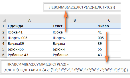
Метод 2: узнать позицию 1- й цифры в строке
Альтернативное решение — использовать эту формулу массива для определения позиции первой цифры:
{=МИН(ПОИСК({0;1;2;3;4;5;6;7;8;9};A2&»0123456789″))}
Как видите, мы последовательно ищем каждое число из массива {0,1,2,3,4,5,6,7,8,9}. Чтобы избежать появления ошибки если цифра не найдена, мы после содержимого ячейки A2 добавляем эти 10 цифр. Excel последовательно перебирает все символы в поисках этих десяти цифр. В итоге получаем опять же массив из 10 цифр — номеров позиций, в которых они нашлись. И из них функция МИН выбирает наименьшее число. Это и будет та позиция, с которой начинается группа чисел, которую нужно отделить от основного содержимого.
Также обратите внимание, что это формула массива и ввод её нужно заканчивать не как обычно, а комбинацией клавиш CTRL + SHIFT + ENTER.
Как только позиция первой цифры найдена, вы можете разделить буквы и числа, используя очень простые формулы ЛЕВСИМВ и ПРАВСИМВ.
Чтобы получить текст:
=ЛЕВСИМВ(A2; B2-1)
Чтобы получить числа:
=ПРАВСИМВ(A2; ДЛСТР(A2)-B2+1)
Где A2 — исходная строка, а B2 — позиция первого числа.
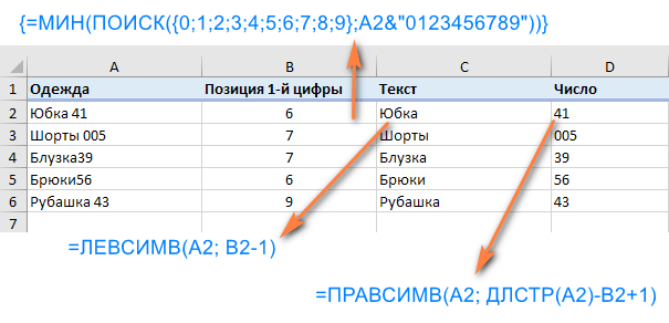
Чтобы избавиться от вспомогательного столбца, в котором мы вычисляли позицию первой цифры, вы можете встроить МИН в функции ЛЕВСИМВ и ПРАВСИМВ:
Для вытаскивания текста:
=ЛЕВСИМВ(A2; МИН(ПОИСК({0;1;2;3;4;5;6;7;8;9};A2&»0123456789″))-1)
Для чисел:
=ПРАВСИМВ(A2; ДЛСТР(A2)-МИН(ПОИСК({0;1;2;3;4;5;6;7;8;9};A2&»0123456789″))+1)
Этого же результата можно достичь и чуть иначе.
Сначала мы извлекаем из ячейки числа при помощи вот такого выражения:
=ПРАВСИМВ(A2;СУММ(ДЛСТР(A2) -ДЛСТР(ПОДСТАВИТЬ(A2; {«0″;»1″;»2″;»3″;»4″;»5″;»6″;»7″;»8″;»9″};»»))))
То есть, сравниваем длину нашего текста без чисел с его исходной длиной, и получаем количество цифр, которое нужно взять справа. К примеру, если текст без цифр стал короче на 2 символа, значит справа надо «отрезать» 2 символа, которые и будут нашим искомым числом.
А затем уже берём оставшееся:
=ЛЕВСИМВ(A2;ДЛСТР(A2)-ДЛСТР(C2))

Как видите, результат тот же. Можете воспользоваться любым способом.
Как разделить ячейку вида ‘число + текст’.
Если вы разделяете ячейки, в которых буквы стоят после цифр, вы можете отделять числа по следующей формуле:
=ЛЕВСИМВ(A2;СУММ(ДЛСТР(A2) — ДЛСТР(ПОДСТАВИТЬ(A2; {«0″;»1″;»2″;»3″;»4″;»5″;»6″;»7″;»8″;»9″};»»))))
Она аналогична рассмотренной в предыдущем примере, за исключением того, что вы используете функцию ЛЕВСИМВ вместо ПРАВСИМВ, чтобы получить число теперь уже из левой части выражения.
Теперь, когда у вас есть числа, отделите буквы, вычитая количество цифр из общей длины исходной строки:
=ПРАВСИМВ(A2;ДЛСТР(A2)-ДЛСТР(B2))
Где A2 — исходная строка, а B2 — искомое число, как показано на снимке экрана ниже:

Как разбить текст по ячейкам по маске (шаблону).
Эта опция очень удобна, когда вам нужно разбить список схожих строк на некоторые элементы или подстроки. Сложность состоит в том, что исходный текст должен быть разделен не при каждом появлении определенного разделителя (например, пробела), а только при некоторых определенных вхождениях. Следующий пример упрощает понимание.
Предположим, у вас есть список строк, извлеченных из некоторого файла журнала:

Вы хотите, чтобы дата и время, если таковые имеются, код ошибки и поясняющие сведения были размещены в 3 отдельных столбцах. Вы не можете использовать пробел в качестве разделителя, потому что между датой и временем также есть пробелы. Также есть пробелы в тексте пояснения, который также должен весь находиться слитно в одном столбце.
Решением является разбиение строки по следующей маске: * ERROR: * Exception: *
Здесь звездочка (*) представляет любое количество символов.
Двоеточия (:) включены в разделители, потому что мы не хотим, чтобы они появлялись в результирующих ячейках.
То есть в данном случае в качестве разделителя по столбцам выступают не отдельные символы, а целые слова.
Итак, в начале ищем позицию первого разделителя.
=ПОИСК(«ERROR:»;A2;1)
Затем аналогичным образом находим позицию, в которой начинается второй разделитель:
=ПОИСК(«Exception:»;A2;1)
Итак, для ячейки A2 шаблон выглядит следующим образом:
С 1 по 20 символ – дата и время. С 21 по 26 символ – разделитель “ERROR:”. Далее – код ошибки. С 31 по 40 символ – второй разделитель “Exception:”. Затем следует описание ошибки.
Таким образом, в первый столбец мы поместим первые 20 знаков:
=—ЛЕВСИМВ(A2;ПОИСК(«ERROR:»;A2;1)-1)
Обратите внимание, что мы взяли на 1 позицию меньше, чем начало первого разделителя. Кроме того, чтобы сразу конвертировать всё это в дату, ставим перед формулой два знака минус. Это автоматически преобразует цифры в число, а дата как раз и хранится в виде числа. Остается только установить нужный формат даты и времени стандартными средствами Excel.
Далее нужно получить код:
=ПСТР(A2;ПОИСК(«ERROR:»;A2;1)+6;ПОИСК(«Exception:»;A2;1)-(ПОИСК(«ERROR:»;A2;1)+6))
Думаю, вы понимаете, что 6 – это количество знаков в нашем слове-разделителе «ERROR:».
Ну и, наконец, выделяем из этой фразы пояснение:
=ПРАВСИМВ(A2;ДЛСТР(A2)-(ПОИСК(«Exception:»;A2;1)+10))
Аналогично добавляем 10 к найденной позиции второго разделителя «Exception:», чтобы выйти на координаты первого символа сразу после разделителя. Ведь функция говорит нам только то, где разделитель начинается, а не заканчивается.
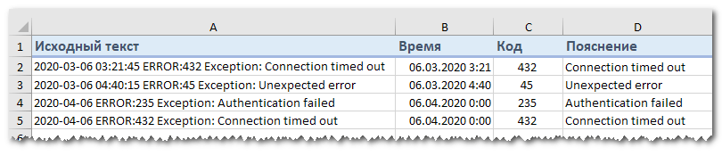
Таким образом, ячейку мы распределили по 3 столбцам, исключив при этом слова-разделители.
Если выяснение загадочных поворотов формул Excel — не ваше любимое занятие, вам может понравиться визуальный метод разделения ячеек в Excel, который демонстрируется в следующей части этого руководства.
Как разделить ячейки в Excel с помощью функции разделения текста Split Text.
Альтернативный способ разбить столбец в Excel — использовать функцию разделения текста, включенную в надстройку Ultimate Suite for Excel. Она предоставляет следующие возможности:
- Разделить ячейку по символу-разделителю.
- Разделить ячейку по нескольким разделителям.
- Разделить ячейку по маске (шаблону).
Чтобы было понятнее, давайте более подробно рассмотрим каждый вариант по очереди.
Разделить ячейку по символу-разделителю.
Выбирайте этот вариант, если хотите разделить содержимое ячейки при каждом появлении определённого символа .
Для этого примера возьмем строки шаблона Товар-Цвет-Размер , который мы использовали в первой части этого руководства. Как вы помните, мы разделили их на 3 разных столбца, используя 3 разные формулы . А вот как добиться того же результата за 2 быстрых шага:
- Предполагая, что у вас установлен Ultimate Suite , выберите ячейки, которые нужно разделить, и щелкните значок «Разделить текст (Split Text)» на вкладке «Ablebits Data».
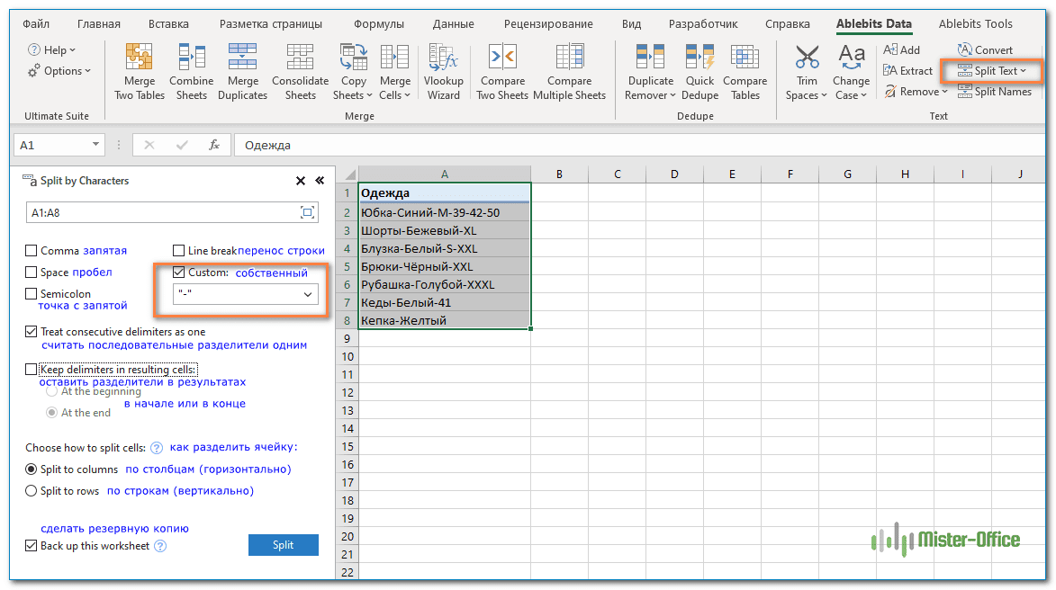
- Панель Разделить текст откроется в правой части окна Excel, и вы выполните следующие действия:
- Разверните группу «Разбить по символам (Split by Characters)» и выберите один из предопределенных разделителей или введите любой другой символ в поле «Пользовательский (Custom)» .
- Выберите, как именно разбивать ячейки: по столбцам или строкам.
- Нажмите кнопку «Разделить (Split)» .
Примечание. Если в ячейке может быть несколько последовательных разделителей (например, более одного символа пробела подряд), установите флажок « Считать последовательные разделители одним».
Готово! Задача, которая требовала 3 формул и 5 различных функций, теперь занимает всего пару секунд и одно нажатие кнопки.

Разделить ячейку по нескольким разделителям.
Этот параметр позволяет разделять текстовые ячейки, используя любую комбинацию символов в качестве разделителя. Технически вы разделяете строку на части, используя одну или несколько разных подстрок в качестве границ.
Например, чтобы разделить предложение на части, используя запятые и союзы, активируйте инструмент «Разбить по строкам (Split by Strings)» и введите разделители, по одному в каждой строке:

В данном случае в качестве разделителей мы используем запятую и союз “или”.
В результате исходная фраза разделяется при появлении любого разделителя:

Примечание. Союзы «или», а также «и» часто могут быть частью слова в вашей исследуемой фразе, так что не забудьте ввести пробел до и после них, чтобы предотвратить разрывы слов на части.
А вот еще один пример. Предположим, вы импортировали столбец дат из внешнего источника, и выглядит он следующим образом:
5.1.2021 12:20
9.8.2021 14:50
Этот формат не является обычным для Excel, и поэтому ни одна из функций даты не распознает здесь какие-либо элементы даты или времени. Чтобы разделить день, месяц, год, часы и минуты на отдельные ячейки, введите следующие символы в поле Spilt by strings:
- Точка (.) Для разделения дня, месяца и года
- Двоеточие (:) для разделения часов и минут
- Пробел для разграничения даты и времени

Нажмите кнопку Split, и вы сразу получите результат:
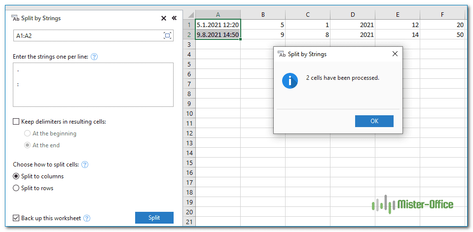
Разделить ячейки по маске (шаблону).
Эта опция очень удобна, когда вам нужно разбить список однородных строк на некоторые элементы или подстроки.
Сложность заключается в том, что исходный текст не может быть разделен при каждом появлении заданного разделителя, а только при некоторых определенных вхождениях. Следующий пример упростит понимание.
Предположим, у вас есть список строк, извлеченных из некоторого файла журнала. Чуть выше в этой статье мы разбивали этот текст по ячейкам при помощи формул. А сейчас используем специальный инструмент. И вы сами решите, какой из способов удобнее и проще.
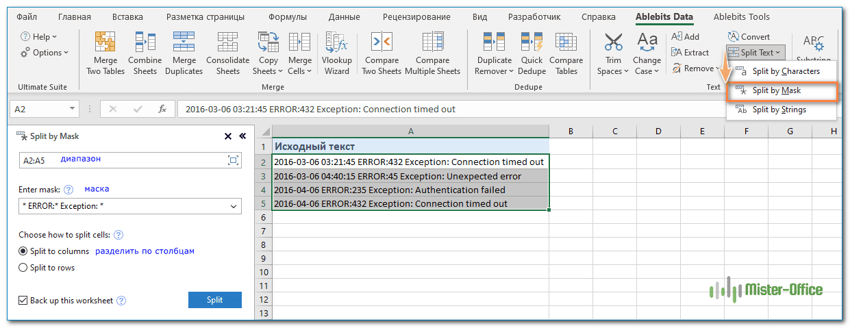
Вы хотите, чтобы дата и время, если таковые имеются, код ошибки и пояснительная информация, были в трех отдельных столбцах. Вы не можете использовать пробел в качестве разделителя, потому что между датой и временем имеются пробелы, которые должны отображаться в одном столбце, и есть пробелы в тексте пояснения, который также должен быть расположен в отдельном столбце.
Решением является разбиение строки по следующей маске:
* ERROR:* Exception: *
Где звездочка (*) представляет любое количество символов.
Двоеточия (:) включены в разделители, потому что мы не хотим, чтобы они появлялись в результирующих ячейках.
А теперь нажмите кнопку «Разбить по маске (Split by Mask)» на панели «Split Text» , введите маску в соответствующее поле и нажмите «Split».
Результат будет примерно таким:

Примечание. При разделении строки по маске учитывается регистр. Поэтому не забудьте ввести символы в шаблоне точно так, как они отображаются в исходных данных.
Большое преимущество этого метода — гибкость. Например, если все исходные строки имеют значения даты и времени, и вы хотите, чтобы они отображались в разных столбцах, используйте эту маску:
* * ERROR:* Exception: *
Проще говоря, маска указывает надстройке разделить исходные строки на 4 части:
- Все символы перед 1-м пробелом в строке (дата)
- Символы между 1-м пробелом и словом ERROR: (время)
- Текст между ERROR: и Exception: (код ошибки)
- Все, что идет после Exception: (текст описания)

Думаю, вы согласитесь, что использование надстройки Split Text гораздо быстрее и проще, нежели использование формул.
Надеюсь, вам понравился этот быстрый и простой способ разделения строк в Excel. Если вам интересно попробовать, ознакомительная версия доступна для загрузки здесь.
Вот как вы можете разделить текст по ячейкам таблицы Excel, используя различные комбинации функций, а также специальные инструменты. Благодарю вас за чтение и надеюсь увидеть вас в нашем блоге на следующей неделе!
Читайте также:
 Поиск ВПР нескольких значений по нескольким условиям — В статье показаны способы поиска (ВПР) нескольких значений в Excel на основе одного или нескольких условий и возврата нескольких результатов в столбце, строке или в отдельной ячейке. При использовании Microsoft…
  Формат времени в Excel — Вы узнаете об особенностях формата времени Excel, как записать его в часах, минутах или секундах, как перевести в число или текст, а также о том, как добавить время с помощью…
  Как сделать диаграмму Ганта — Думаю, каждый пользователь Excel знает, что такое диаграмма и как ее создать. Однако один вид графиков остается достаточно сложным для многих — это диаграмма Ганта. В этом кратком руководстве я постараюсь показать…
  Как сделать автозаполнение в Excel — В этой статье рассматривается функция автозаполнения Excel. Вы узнаете, как заполнять ряды чисел, дат и других данных, создавать и использовать настраиваемые списки в Excel. Эта статья также позволяет вам убедиться, что вы…
  Функция ИНДЕКС в Excel — 6 примеров использования — В этом руководстве вы найдете ряд примеров формул, демонстрирующих наиболее эффективное использование ИНДЕКС в Excel. Из всех функций Excel, возможности которых часто недооцениваются и используются недостаточно, ИНДЕКС определенно занимает место…
  Быстрое удаление пустых столбцов в Excel — В этом руководстве вы узнаете, как можно легко удалить пустые столбцы в Excel с помощью макроса, формулы и даже простым нажатием кнопки. Как бы банально это ни звучало, удаление пустых…
Bottom Line: Learn how to use formulas and functions in Excel to split full names into columns of first and last names.
Skill Level: Intermediate
Watch the Tutorial
Download the Excel Files
You can download both the before and after files below. The before file is so you can follow along, and the after file includes all of the formulas already written.
Splitting Text Into Separate Columns
We’ve been talking about various ways to take the text that is in one column and divide it into two. Specifically, we’ve been looking at the common example of taking a Full Name column and splitting it into First Name and Last Name.
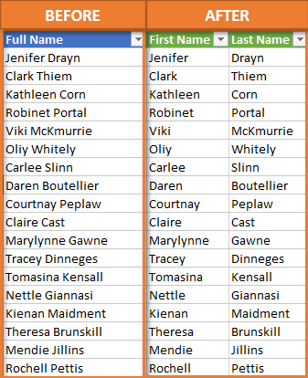
The first solution we looked at used Power Query and you can view that tutorial here: How to Split Cells and Text in Excel with Power Query. Then we explored how to use the Text to Columns feature that’s built into Excel: Split Cells with Text to Columns in Excel. Today, I want to show you how to accomplish the same thing with formulas.
Using 4 Functions to Build our Formulas
To split our Full Name column into First and Last using formulas, we need to use four different functions. We’ll be using SEARCH and LEFT to pull out the first name. Then we’ll use LEN and RIGHT to pull out the last name.
The SEARCH Function
They key to breaking up the first names from the last names is for Excel to identify what all of the full names have in common. That common factor is the space character that separates the two names. To help our formula identify everything to the left of that space character as the first name, we need to use the SEARCH function.
The SEARCH function returns the number of the character at which a specific character or text string is found, reading left to right. In other words, what number is the space character in the line of characters that make up a full name? In my name, Jon Acampora, the space character is the 4th character (after J, o, and n), so the SEARCH function returns the number 4.
There are three arguments for SEARCH.
- The first argument for the SEARCH function is find_text. The text we want to find in our entries is the space character. So, for find_text, we enter ” “, being sure to include the quotation marks.
- The second argument is within_text. This is the text we are searching in for the space character. That would be the cell that has the full name. In our example, the first cell that has a full name is A2. Since we are working with Excel Tables, the formula will copy down and change to B2, C2, etc., for each respective row.
- The third and last argument is [start_num]. This argument is for cases where you want to ignore a certain number of characters in the text before beginning your search. In our case, we want to search the entire text, beginning with the very first character, so we do not need to define this argument.
All together, our formula reads: =SEARCH(” “,A2)
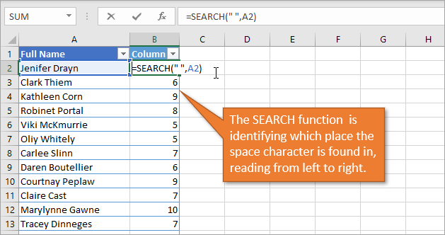
I started with the SEARCH function because it will be used as one of the arguments for the next function we’re going to look at. That is the LEFT function,
The LEFT Function
The LEFT function returns the specified number of characters from the start of a text string. To specify that number, we will use the value we just identified with the SEARCH function. The LEFT function will pull out the letters from the left of the Full Name column.
The LEFT function has two arguments.
- The first argument is text. That is just the cell that the function is pulling from—in our case A2.
- The second argument is [num_chars]. This is the number of characters that the function should pull. For this argument, we will use the formula we created above and subtract 1 from it, because we don’t want to actually include the space character in our results. So for our example, this argument would be SEARCH(” “,A2)-1
All together, our formula reads =LEFT(A2,SEARCH(” “,A2)-1)
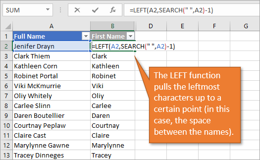
Now that we’ve extracted the first name using the LEFT function, you can guess how we’re going to use the RIGHT function. It will pull out the last name. But before we go there, let me explain one of the components that we will need for that formula. That is the LEN function.
The LEN Function
LEN stands for LENGTH. This function returns the number of characters in a text string. In my name, there are 12 characters: 3 for Jon, 8 for Acampora, and 1 for the space in between.
There is only one argument for LEN, and that is to identify which text to count characters from. For our example, we again are using A2 for the Full Name. Our formula is simply =LEN(A2)
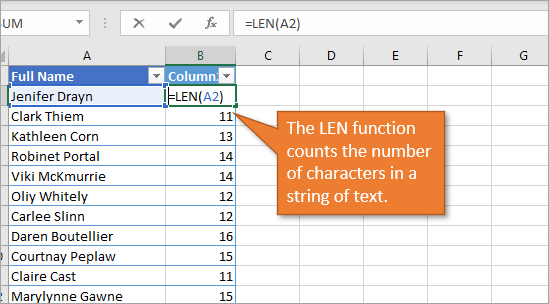
The RIGHT Function
The RIGHT formula returns the specified number of characters from the end of a text string. RIGHT has two arguments.
- The first argument is text. This is the text that it is looking through in order to return the right characters. Just as with the LEFT function above, we are looking at cell A2.
- The second argument is [num_chars]. For this argument we want to subtract the number of characters that we identified using the SEARCH function from the total number of characters that we identified with the LEN function. That will give us the number of characters in the last name.
Our formula, all together, is =RIGHT(A2,LEN(A2)-SEARCH(” “,A2))
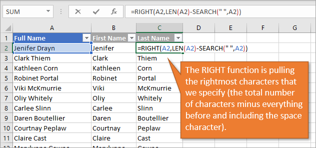
Note that we did not subtract 1 like we did before, because we want the space character included in the number that is being deducted from the total length.
Pros and Cons for Using Formulas to Split Cells
The one outstanding advantage to this method for splitting text is the automatic updates. When edits, additions, or deletions are made to the Full Name column, the First and Last names change as well. This is a big benefit compared to using Text to Columns, which requires you to completely repeat the process when changes are made. And even the Power Query method, though much simpler to update than Text to Columns, still requires a refresh to be manually selected.
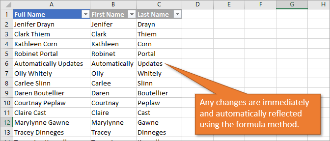
Of course, one obvious disadvantage to this technique is that even though each of the four functions are relatively simple to understand, it takes some thought and time to combine them all and create formulas that work correctly. In other words, is not the easiest solution to implement of the three methods presented thus far.
Another disadvantage to consider is the fact that this only works for scenarios that have two names in the Full Name column. If you have data that includes middle names or two first names, the formula method isn’t helpful without making some considerable modifications to the formulas. (Homework challenge! If you’d like to give that a try, please do so and let us know your results in the comments.) As we saw in the Power Query tutorial, you do in fact have the capability to pull out more than two names with that technique.
Here are the links to the other posts on ways to split text:
- Split Cells with Text to Columns in Excel
- How to Split Text in Cells with Flash Fill in Excel
- How to Split Cells and Text in Excel with Power Query
- Split by Delimiter into Rows (and Columns) with Power Query
Conclusion
I hope you’ve learned something new from this post and that is helpful as you split data into separate columns. If you have questions or remarks, please leave a comment below!
Содержание
- Split a cell
- Split the content from one cell into two or more cells
- Distribute the contents of a cell into adjacent columns
- Need more help?
- How to Split Text in Cells Using Formulas
- Watch the Tutorial
- Download the Excel Files
- Splitting Text Into Separate Columns
- Using 4 Functions to Build our Formulas
- The SEARCH Function
- The LEFT Function
- The LEN Function
- The RIGHT Function
- Pros and Cons for Using Formulas to Split Cells
- Ways to Split Text
- Conclusion
- Divide text in multiple lines in a single Excel cell using VBA
- 2 Answers 2
- How to split text string in Excel by comma, space, character or mask
- How to split text in Excel using formulas
- Split string by comma, semicolon, slash, dash or other delimiter
- How to split string by line break in Excel
- How to split text and numbers in Excel
- Split string of ‘text + number’ pattern
- Method 1: Count digits and extract that many chars
- Method 2: Find out the position of the 1 st digit in a string
- Split string of ‘number + text’ pattern
- How to split cells in Excel with Split Text tool
- Split cells by character
- Split cells by string
- Split cells by mask (pattern)
Split a cell
You might want to split a cell into two smaller cells within a single column. Unfortunately, you can’t do this in Excel. Instead, create a new column next to the column that has the cell you want to split and then split the cell. You can also split the contents of a cell into multiple adjacent cells.
See the following screenshots for an example:
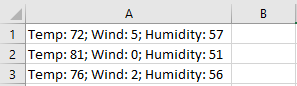
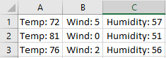
Split the content from one cell into two or more cells
Note: Excel for the web doesn’t have the Text to Columns Wizard. Instead, you can Split text into different columns with functions.
Select the cell or cells whose contents you want to split.
Important: When you split the contents, they will overwrite the contents in the next cell to the right, so make sure to have empty space there.
On the Data tab, in the Data Tools group, click Text to Columns. The Convert Text to Columns Wizard opens.
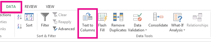
Choose Delimited if it is not already selected, and then click Next.
Select the delimiter or delimiters to define the places where you want to split the cell content. The Data preview section shows you what your content would look like. Click Next.
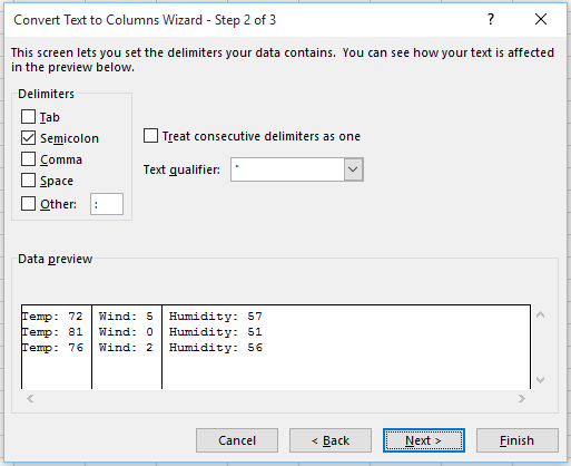
In the Column data format area, select the data format for the new columns. By default, the columns have the same data format as the original cell. Click Finish.
Источник
Distribute the contents of a cell into adjacent columns
You can divide the contents of a cell and distribute the constituent parts into multiple adjacent cells. For example, if your worksheet contains a column Full Name, you can split that column into two columns—a First Name column and Last Name column.
For an alternative method of distributing text across columns, see the article, Split text among columns by using functions.
You can combine cells with the CONCAT function or the CONCATENATE function.
Follow these steps:
Note: A range containing a column that you want to split can include any number of rows, but it can include no more than one column. It’s important to keep enough blank columns to the right of the selected column, which will prevent data in any adjacent columns from being overwritten by the data that is to be distributed. If necessary, insert a number of empty columns that will be sufficient to contain each of the constituent parts of the distributed data.
Select the cell, range, or entire column that contains the text values that you want to split.
On the Data tab, in the Data Tools group, click Text to Columns.
Follow the instructions in the Convert Text to Columns Wizard to specify how you want to divide the text into separate columns.
Note: For help with completing all the steps of the wizard, see the topic, Split text into different columns with the Convert Text to Columns Wizard, or click Help  in the Convert to Text Columns Wizard.
This feature isn’t available in Excel for the web.
If you have the Excel desktop application, you can use the Open in Excel button to open the workbook and distribute the contents of a cell into adjacent columns.
Need more help?
You can always ask an expert in the Excel Tech Community or get support in the Answers community.
Источник
How to Split Text in Cells Using Formulas
Bottom Line: Learn how to use formulas and functions in Excel to split full names into columns of first and last names.
Skill Level: Intermediate
Watch the Tutorial
Download the Excel Files
You can download both the before and after files below. The before file is so you can follow along, and the after file includes all of the formulas already written.
Split-Names-with-Formulas-BEGIN.xlsx
Split-Names-with-Formulas-FINAL.xlsx
Splitting Text Into Separate Columns
We’ve been talking about various ways to take the text that is in one column and divide it into two. Specifically, we’ve been looking at the common example of taking a Full Name column and splitting it into First Name and Last Name.
The first solution we looked at used Power Query and you can view that tutorial here: How to Split Cells and Text in Excel with Power Query. Then we explored how to use the Text to Columns feature that’s built into Excel: Split Cells with Text to Columns in Excel. Today, I want to show you how to accomplish the same thing with formulas.
Using 4 Functions to Build our Formulas
To split our Full Name column into First and Last using formulas, we need to use four different functions. We’ll be using SEARCH and LEFT to pull out the first name. Then we’ll use LEN and RIGHT to pull out the last name.
The SEARCH Function
They key to breaking up the first names from the last names is for Excel to identify what all of the full names have in common. That common factor is the space character that separates the two names. To help our formula identify everything to the left of that space character as the first name, we need to use the SEARCH function.
The SEARCH function returns the number of the character at which a specific character or text string is found, reading left to right. In other words, what number is the space character in the line of characters that make up a full name? In my name, Jon Acampora, the space character is the 4th character (after J, o, and n), so the SEARCH function returns the number 4.
There are three arguments for SEARCH.
- The first argument for the SEARCH function is find_text. The text we want to find in our entries is the space character. So, for find_text, we enter ” “, being sure to include the quotation marks.
- The second argument is within_text. This is the text we are searching in for the space character. That would be the cell that has the full name. In our example, the first cell that has a full name is A2. Since we are working with Excel Tables, the formula will copy down and change to B2, C2, etc., for each respective row.
- The third and last argument is [start_num]. This argument is for cases where you want to ignore a certain number of characters in the text before beginning your search. In our case, we want to search the entire text, beginning with the very first character, so we do not need to define this argument.
All together, our formula reads: =SEARCH(” “,A2)
I started with the SEARCH function because it will be used as one of the arguments for the next function we’re going to look at. That is the LEFT function,
The LEFT Function
The LEFT function returns the specified number of characters from the start of a text string. To specify that number, we will use the value we just identified with the SEARCH function. The LEFT function will pull out the letters from the left of the Full Name column.
The LEFT function has two arguments.
- The first argument is text. That is just the cell that the function is pulling from—in our case A2.
- The second argument is [num_chars]. This is the number of characters that the function should pull. For this argument, we will use the formula we created above and subtract 1 from it, because we don’t want to actually include the space character in our results. So for our example, this argument would be SEARCH(” “,A2)-1
All together, our formula reads =LEFT(A2,SEARCH(” “,A2)-1)
Now that we’ve extracted the first name using the LEFT function, you can guess how we’re going to use the RIGHT function. It will pull out the last name. But before we go there, let me explain one of the components that we will need for that formula. That is the LEN function.
The LEN Function
LEN stands for LENGTH. This function returns the number of characters in a text string. In my name, there are 12 characters: 3 for Jon, 8 for Acampora, and 1 for the space in between.
There is only one argument for LEN, and that is to identify which text to count characters from. For our example, we again are using A2 for the Full Name. Our formula is simply =LEN(A2)
The RIGHT Function
The RIGHT formula returns the specified number of characters from the end of a text string. RIGHT has two arguments.
- The first argument is text. This is the text that it is looking through in order to return the right characters. Just as with the LEFT function above, we are looking at cell A2.
- The second argument is [num_chars]. For this argument we want to subtract the number of characters that we identified using the SEARCH function from the total number of characters that we identified with the LEN function. That will give us the number of characters in the last name.
Our formula, all together, is =RIGHT(A2,LEN(A2)-SEARCH(” “,A2))
Note that we did not subtract 1 like we did before, because we want the space character included in the number that is being deducted from the total length.
Pros and Cons for Using Formulas to Split Cells
The one outstanding advantage to this method for splitting text is the automatic updates. When edits, additions, or deletions are made to the Full Name column, the First and Last names change as well. This is a big benefit compared to using Text to Columns, which requires you to completely repeat the process when changes are made. And even the Power Query method, though much simpler to update than Text to Columns, still requires a refresh to be manually selected.
Of course, one obvious disadvantage to this technique is that even though each of the four functions are relatively simple to understand, it takes some thought and time to combine them all and create formulas that work correctly. In other words, is not the easiest solution to implement of the three methods presented thus far.
Another disadvantage to consider is the fact that this only works for scenarios that have two names in the Full Name column. If you have data that includes middle names or two first names, the formula method isn’t helpful without making some considerable modifications to the formulas. (Homework challenge! If you’d like to give that a try, please do so and let us know your results in the comments.) As we saw in the Power Query tutorial, you do in fact have the capability to pull out more than two names with that technique.
Ways to Split Text
Here are the links to the other posts on ways to split text:
Conclusion
I hope you’ve learned something new from this post and that is helpful as you split data into separate columns. If you have questions or remarks, please leave a comment below!
Источник
Divide text in multiple lines in a single Excel cell using VBA
So i’ve been searching how to divide text depending on its length but couldn’t find anything.
My question is : In Excel using vba code, is it possible to divide a line of text into several lines in a single cell?
I don’t have access to the text itself, it’s inserted via a query from an Access Database. This being said, I can’t really use the linebreak character «Chr(10)» to help me out.
I’m thinking of a way to distinguish if the text length is greater than a certain number of letters, it could be splited in 2 (or more actually) and then concatonate it using the linebreak character.
I hope my question/request is clear enough.
Thanks in advance.
2 Answers 2
If it’s just for display purposes, then I think there is an easier method. You could set the column width to a width you like and format the cells in that column to Wrap Text.
There are two settings on your Querytable that you need to pay attention to. «Adjust column width» is unchecked by default and you need to check it. If you don’t, Excel will make the column bigger and the fact that you have Wrap Text checked won’t matter. «Preserve cell formatting» is checked by default and needs to remain checked. That will ensure that Wrap text stays checked for that column.
Setting the column width won’t guarantee that you get a specific number of characters unless you use a fixed font. But if you just want to get close, this should work.
Источник
How to split text string in Excel by comma, space, character or mask
 by Svetlana Cheusheva, updated on February 7, 2023
The tutorial explains how to split cells in Excel using formulas and the Split Text feature. You will learn how to separate text by comma, space or any other delimiter, and how to split strings into text and numbers.
Splitting text from one cell into several cells is the task all Excel users are dealing with once in a while. In one of our earlier articles, we discussed how to split cells in Excel using the Text to Column feature and Flash Fill. Today, we are going to take an in-depth look at how you can split strings using formulas and the Split Text tool.
How to split text in Excel using formulas
To split string in Excel, you generally use the LEFT, RIGHT or MID function in combination with either FIND or SEARCH. At first sight, some of the formulas might look complex, but the logic is in fact quite simple, and the following examples will give you some clues.
Split string by comma, semicolon, slash, dash or other delimiter
When splitting cells in Excel, the key is to locate the position of the delimiter within the text string. Depending on your task, this can be done by using either case-insensitive SEARCH or case-sensitive FIND. Once you have the delimiter’s position, use the RIGHT, LEFT or MID function to extract the corresponding part of the text string. For better understanding, let’s consider the following example.
Supposing you have a list of SKUs of the Item-Color-Size pattern, and you want to split the column into 3 separate columns: 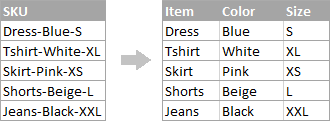
- To extract the item name (all characters before the 1st hyphen), insert the following formula in B2, and then copy it down the column:
In this formula, SEARCH determines the position of the 1st hyphen («-«) in the string, and the LEFT function extracts all the characters left to it (you subtract 1 from the hyphen’s position because you don’t want to extract the hyphen itself). 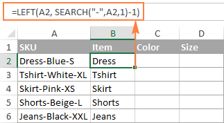
To extract the color (all characters between the 1st and 2nd hyphens), enter the following formula in C2, and then copy it down to other cells:
=MID(A2, SEARCH(«-«,A2) + 1, SEARCH(«-«,A2,SEARCH(«-«,A2)+1) — SEARCH(«-«,A2) — 1) 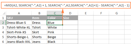
In this formula, we are using the Excel MID function to extract text from A2.
The starting position and the number of characters to be extracted are calculated with the help of 4 different SEARCH functions:
- Start number is the position of the first hyphen +1:
SEARCH(«-«,A2) + 1
Number of characters to extract: the difference between the position of the 2 nd hyphen and the 1 st hyphen, minus 1:
SEARCH(«-«, A2, SEARCH(«-«,A2)+1) — SEARCH(«-«,A2) -1
To extract the size (all characters after the 3rd hyphen), enter the following formula in D2:
=RIGHT(A2,LEN(A2) — SEARCH(«-«, A2, SEARCH(«-«, A2) + 1))
In this formula, the LEN function returns the total length of the string, from which you subtract the position of the 2 nd hyphen. The difference is the number of characters after the 2 nd hyphen, and the RIGHT function extracts them. 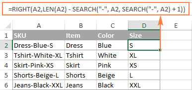
In a similar fashion, you can split column by any other character. All you have to do is to replace «-» with the required delimiter, for example space (» «), comma («,»), slash («/»), colon («;»), semicolon («;»), and so on.
Tip. In the above formulas, +1 and -1 correspond to the number of characters in the delimiter. In this example, it’s a hyphen (1 character). If your delimiter consists of 2 characters, e.g. a comma and a space, then supply only the comma («,») to the SEARCH function, and use +2 and -2 instead of +1 and -1.
How to split string by line break in Excel
To split text by space, use formulas similar to the ones demonstrated in the previous example. The only difference is that you will need the CHAR function to supply the line break character since you cannot type it directly in the formula.
Supposing, the cells you want to split look similar to this: 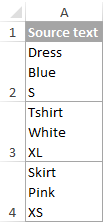
Take the formulas from the previous example and replace a hyphen («-«) with CHAR(10) where 10 is the ASCII code for Line feed.
- To extract the item name:
=LEFT(A2, SEARCH(CHAR(10),A2,1)-1)
To extract the color:
=MID(A2, SEARCH(CHAR(10),A2) + 1, SEARCH(CHAR(10),A2,SEARCH(CHAR(10),A2)+1) — SEARCH(CHAR(10),A2) — 1)
To extract the size:
=RIGHT(A2,LEN(A2) — SEARCH(CHAR(10), A2, SEARCH(CHAR(10), A2) + 1))
And this is how the result looks like: 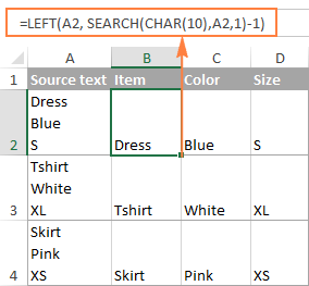
How to split text and numbers in Excel
To begin with, there is no universal solution that would work for all alphanumeric strings. Which formula to use depends on the particular string pattern. Below you will find the formulas for the two common scenarios.
Split string of ‘text + number’ pattern
Supposing, you have a column of strings with text and numbers combined, where a number always follows text. You want to break the original strings so that the text and numbers appear in separate cells, like this: 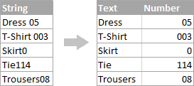
The result may be achieved in two different ways.
Method 1: Count digits and extract that many chars
The easiest way to split text string where number comes after text is this:
To extract numbers, you search the string for every possible number from 0 to 9, get the numbers total, and return that many characters from the end of the string.
With the original string in A2, the formula goes as follows:
To extract text, you calculate how many text characters the string contains by subtracting the number of extracted digits (C2) from the total length of the original string in A2. After that, you use the LEFT function to return that many characters from the beginning of the string.
Where A2 is the original string, and C2 is the extracted number, as shown in the screenshot: 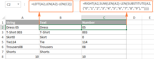
Method 2: Find out the position of the 1 st digit in a string
An alternative solution would be using the following formula to determine the position of the first digit in the string:
Once the position of the first digit is found, you can split text and numbers by using very simple LEFT and RIGHT formulas.
To extract text:
To extract number:
Where A2 is the original string, and B2 is the position of the first number. 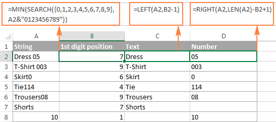
To get rid of the helper column holding the position of the first digit, you can embed the MIN formula into the LEFT and RIGHT functions:
Formula to extract text:
Formula to extract numbers:
Split string of ‘number + text’ pattern
If you are splitting cells where text appears after number, you can extract numbers with the following formula:
The formula is similar to the one discussed in the previous example, except that you use the LEFT function instead of RIGHT to get the number from the left side of the string.
Once you have the numbers, extract text by subtracting the number of digits from the total length of the original string:
Where A2 is the original string and B2 is the extracted number, as shown in the screenshot below: 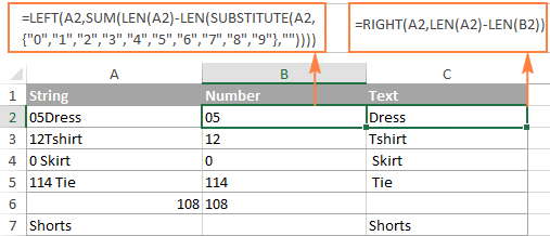
Tip. To get number from any position in a text string, use either this formula or the Extract tool. Or you can create a custom function to split numbers and text into separate columns.
This is how you can split strings in Excel using different combinations of different functions. As you see, the formulas are far from obvious, so you may want to download the sample Excel Split Cells workbook to examine them closer.
If figuring out the arcane twists of Excel formulas is not your favorite occupation, you may like the visual method to split cells in Excel, which is demonstrated in the next part of this tutorial.
How to split cells in Excel with Split Text tool
An alternative way to split a column in Excel is using the Split Text feature included with our Ultimate Suite for Excel, which provides the following options:
To make things clearer, let’s have a closer look at each option, one at a time.
Split cells by character
Choose this option whenever you want to split the cell contents at each occurrence of the specified character.
For this example, let’s the take the strings of the Item-Color-Size pattern that we used in the first part of this tutorial. As you may remember, we separated them into 3 different columns using 3 different formulas. And here’s how you can achieve the same result in 2 quick steps:
- Assuming you have Ultimate Suite installed, select the cells to split, and click the Split Text icon on the Ablebits Data tab.
- The Split Text pane will open on the right side of your Excel window, and you do the following:
- Expand the Split by character group, and select one of the predefined delimiters or type any other character in the Custom box.
- Choose whether to split cells to columns or rows.
- Review the result under the Preview section, and click the Split button.
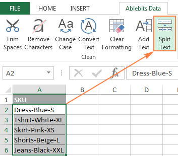
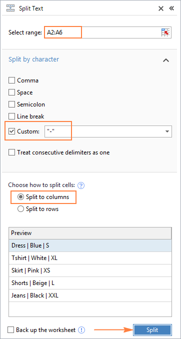
Tip. If there might be several successive delimiters in a cell (for example, more than one space character), select the Treat consecutive delimiters as one box.
Done! The task that required 3 formulas and 5 different functions now only takes a couple of seconds and a button click. 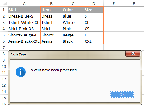
Split cells by string
This option lets you split strings using any combination of characters as a delimiter. Technically, you split a string into parts by using one or several different substrings as the boundaries of each part.
For example, to split a sentence by the conjunctions «and» and «or«, expand the Split by strings group, and enter the delimiter strings, one per line: 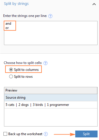
As the result, the source phrase is separated at each occurrence of each delimiter: 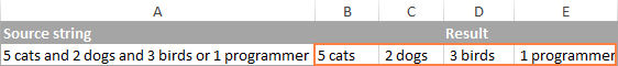
Tip. The characters «or» as well as «and» can often be part of words like «orange» or «Andalusia», so be sure to type a space before and after and and or to prevent splitting words.
And here another, real-life example. Supposing you’ve imported a column of dates from an external source, which look as follows:
This format is not conventional for Excel, and therefore none of the Date functions would recognize any of the date or time elements. To split day, month, year, hours and minutes into separate cells, enter the following characters in the Split by strings box:
- Dot (.) to separate day, month, and year
- Colon (:) to separate hours and minutes
- Space to separate date and time
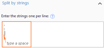
Hit the Split button, and you will immediately get the result: 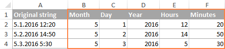
Split cells by mask (pattern)
Separating a cell by mask means splitting a string based on a pattern.
This option comes in very handy when you need to split a list of homogeneous strings into some elements, or substrings. The complication is that the source text cannot be split at each occurrence of a given delimiter, only at some specific occurrence(s). The following example will make things easier to understand.
Supposing you have a list of strings extracted from some log file: 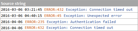
What you want is to have date and time, if any, error code and exception details in 3 separate columns. You cannot utilize a space as the delimiter because there are spaces between date and time, which should appear in one column, and there are spaces within the exception text, which should also appear in one column.
The solution is splitting a string by the following mask: *ERROR:*Exception:*
Where the asterisk (*) represents any number of characters.
The colons (:) are included in the delimiters because we don’t want them to appear in the resulting cells.
And now, expand the Split by mask section on the Split Text pane, type the mask in the Enter delimiters box, and click Split: 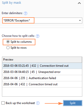
The result will look similar to this: 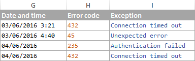
Note. Splitting string by mask is case-sensitive. So, be sure to type the characters in the mask exactly as they appear in the source strings.
A big advantage of this method is flexibility. For example, if all of the original strings have date and time values, and you want them to appear in different columns, use this mask:
Translated into plain English, the mask instructs the add-in to divide the original strings into 4 parts:
- All characters before the 1st space found within the string (date)
- Characters between the 1 st space and the word ERROR: (time)
- Text between ERROR: and Exception: (error code)
- Everything that comes after Exception: (exception text)
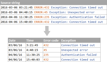
I hope you liked this quick and straightforward way to split strings in Excel. If you are curious to give it a try, an evaluation version is available for download below. I thank you for reading and hope to see you on our blog next week!
Источник
In this guide, we’re going to show you how to split text in Excel by a delimiter.
Download Workbook
We have a sample data which contains concatenated values separated by “|” characters. It is important that the data includes a specific delimiter character between each chunk of data to make splitting text easier.
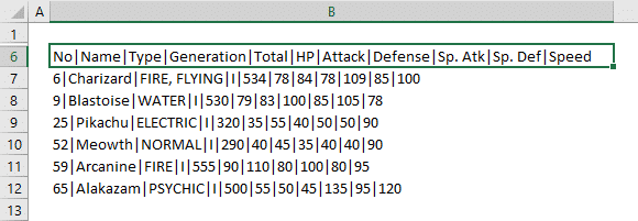
Text to Columns feature for splitting text
When splitting text in Excel, the Text to Columns is one of the most common methods. You can use the Text to Columns feature with all versions of Excel. This feature can split text by a specific character count or delimiter.
- Start with selecting your data. You can use more than one cell in a column.
- Click Data > Text to Columns in the Ribbon.
- On the first step of the wizard, you have 2 options to choose from — these are slicing methods. Since our data in this example is split by delimiters, our choice is going to be Delimited.
- Click Next to continue
- Select the delimiters suitable to your data or choose a character length and click Next.
- Choose corresponding data types for the columns and the destination cell. Please note that if the destination cell is the same cell as where your data is, the original data will be overwritten.
- Click Finish to see the outcome.
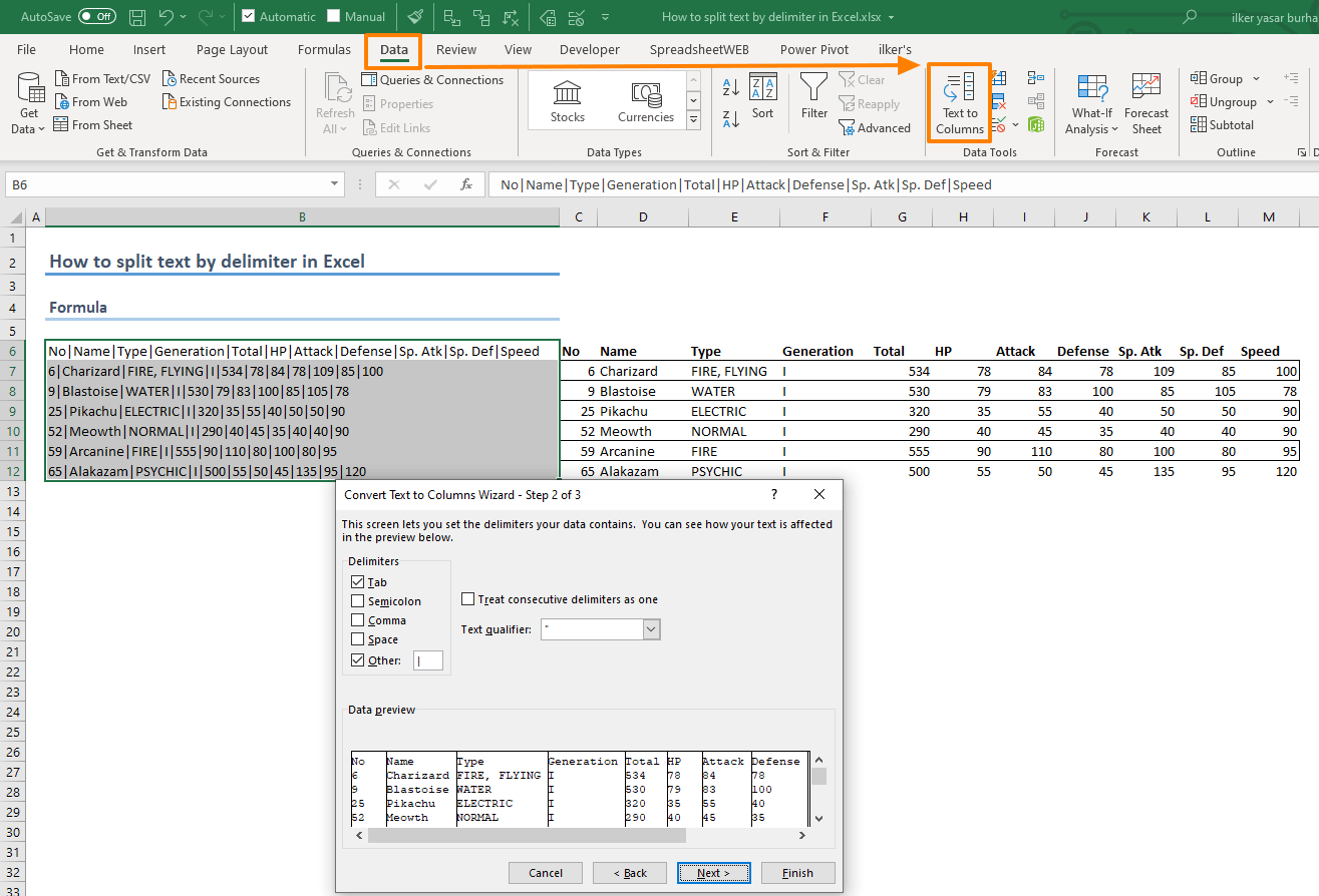
Using formulas to split text
Excel has a variety of text formulas that you can use to locate delimiters and parse data. When using formulas to do so, Excel automatically updates the parsed values when the source is updated.
The formula used in this example uses Microsoft 365’s dynamic array feature, which allows you to populate multiple cells without using array formulas. If you can see the SEQUENCE formula, you can use this method.
Syntax
=TRIM(MID(SUBSTITUTE( text, separator, REPT( “ “, LEN( text ))),(SEQUENCE( 1, column count ) — 1 ) * LEN( text ) + 1,LEN( text )))
How it works
The formula replaces each separator character with space characters first. (see SUBSTITUTE) The number of space characters will be equal to the original string’s character count, which is enough number of spaces to separate each string block (see REPT and LEN).
The SEQUENCE function generates an array of numbers starting with 1, up to the number of maximum columns. Multiplying these sequential numbers with the length of the original string returns character numbers indicating the start of each block.
This approach uses the MID function to parse each string block with given start character number and the number of characters to return. Since the separators are replaced with space characters, each parsed block includes these spaces around the actual string. The TRIM function then removes these spaces.

Flash Fill
The Flash Fill is an Excel tool which can detect the pattern when entering data. A common example is to separate or merge first name and last names. Let’s say column A contains the first name — last name combinations. If you type in the corresponding first name in the same row for column B, Excel shows you a preview for the rest of the column.
Please note that the Flash Fill is available for Excel 2013 and newer versions only.
You can see the same behavior with strings using delimiters to separate data. Just select a cell in the adjacent column and start typing. Occasionally Excel will display a preview. If not, press Ctrl + E like below to split your text.

Power Query
Power Query is a powerful feature, not only for splitting text, but for data management in general. Power Query comes with its own text splitting tool which allows you to split text in multiple ways, like by delimiters, number of characters, or case of letters.
If you are using Excel 2016 or newer — including Microsoft 365 — you can find Power Query options under the Data tab’s Get & Transform section. Excel 2010 and 2013 users should download and install the Power Query as an add-in.
- Select the cells containing the text.
- Click Data > From Sheet. If the data is not in an Excel Table, Excel converts it into an Excel Table first.
- Once the Power Query window is open, find the Split Column under the Transform tab and click to see the options.
- Select the approach that fits your data layout. The data in our example is using By Delimiter since the data is separated by “|”.
- Power Query will show the delimiter character. If you are not seeing the expected delimiter, choose from the list or enter it yourself.
- Click OK to split text.
- If your data includes headers in its first row, like our example does, click Transform > Use First Row as Headers to keep them as headers.
- One you satisfied with the result, click the Home > Close & Load button to move the split data into your workbook.

VBA
VBA is the last text splitting option we want to show in this article. You can use VBA in two ways to split text:
- By calling the Text to Columns feature using VBA,
- Using VBA’s Split function to create array of sub-strings and using a loop to distribute the sub-strings into adjacent cells in the same row.
Text to Columns by VBA
The following code can split data from selected cells into the adjacent columns. Note that each supported delimiter is listed as an argument which you can enable or disable by giving them either True or False. Briefly, True means that you want to set that argument as a delimiter and False means ignore that character.

An easy way to generate a VBA code to split text is to record a macro. Start a recording section using the Record Macro button in the Developer tab, and use the Text to Columns feature. Once the recording is stopped, Excel will save the code for what you did during recording.
The code:
Sub VBATextToColumns_Multiple()
Dim MyRange As Range
Set MyRange = Selection ‘To work on a static range replace Selection via Range object, e.g., Range(“B6:B12”)
MyRange.TextToColumns _
Destination:=MyRange(1, 1).Offset(, 1), _
DataType:=xlDelimited, _
TextQualifier:=xlDoubleQuote, _
ConsecutiveDelimiter:=False, _
Tab:=True, _
SemiColon:=False, _
Comma:=False, _
Space:=False, _
Other:=True, _
OtherChar:=»|»
End Sub
Split Function
Split function can be useful if you want to keep the split blocks in an array. You can only use this method for splitting because of the single delimiter constraint. The following code loops through each cell in a selected column, splits and stores text by the delimiter “|”, and uses another loop to populate the values in the array on cells. The final EntireColumn.AutoFit command adjusts the column widths.

The code:
Sub SplitText()
Dim StringArray() As String, Cell As Range, i As Integer
For Each Cell In Selection ‘To work on a static range replace Selection via Range object, e.g., Range(“B6:B12”)
StringArray = Split(Cell, «|») ‘Change the delimiter with a character suits your data
For i = 0 To UBound(StringArray)
Cell.Offset(, i + 1) = StringArray(i)
Cell.Offset(, i + 1).EntireColumn.AutoFit ‘This is for column width and optional.
Next i
Next
End Sub
This tutorial will demonstrate how to split text strings using a space, comma and more in Excel and Google Sheets.
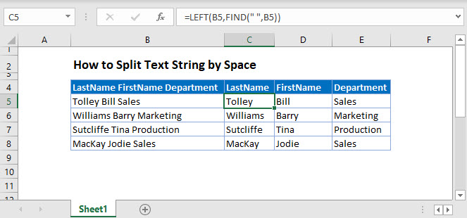
Split Text String with Text to Columns
You can split a text string with the Text to Columns feature in Excel.
Select the text you wish to split.
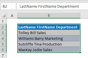
In the Ribbon, select Data>Text to Columns.
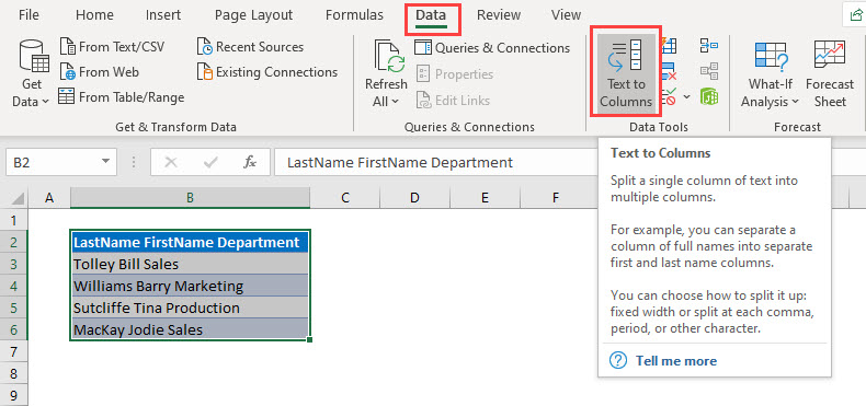
Keep the option “Delimited” selected and click Next.
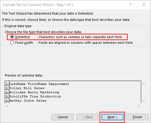
Select “Space” as the Delimiter, and amend the Text qualifier to “None”
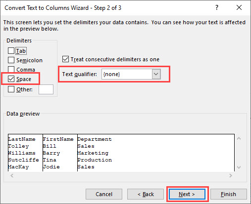
Click Next.
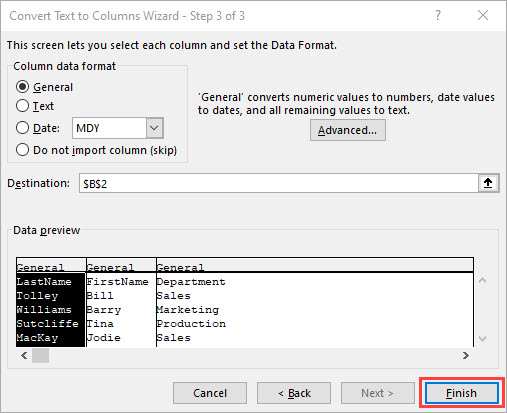
In this step, you can change the data type of the column. Leave them as they are and click Finish.
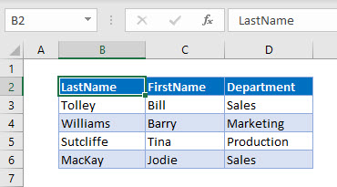
Split Text String by Space
To split a text string at a space or comma, we can use the FIND, LEFT, MID and RIGHT functions.
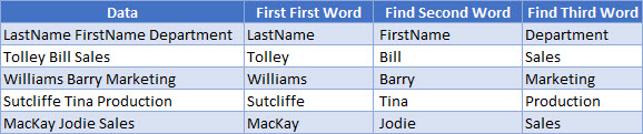
LEFT and FIND Functions
First, we can find the LastName by using the LEFT and FIND functions.
=LEFT(B3, FIND(" " , B3))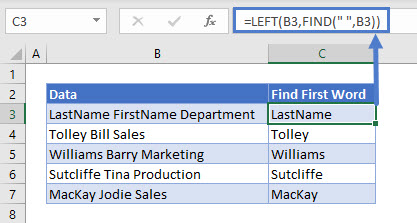
MID and FIND Functions
We can then use the MID and FIND Functions to find the second word in the text string.
=MID(B3,FIND(" ",B3),FIND(" ",B3,FIND(" ",B3)+1)-FIND(" ", B3))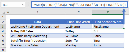
RIGHT and FIND Functions
Finally, we can use the RIGHT, LEN and FIND Functions to find the third word in the text string.
=RIGHT(B3, LEN(B3)-FIND(" ", B3,FIND(" ",B3)+1))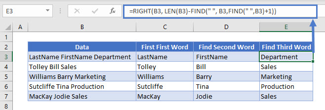
Split Text String by Comma or Other Character
You can use the same formulas to find commas or any other characters in a text string and split the text string accordingly.
The formulas would be slightly different
Find the First word
=LEFT(B3,FIND(",",B3)-1)To find the second word
=MID(B3,FIND(",",B3)+1,FIND(",",B3,FIND(",",B3)+1)-FIND(",", B3)-1)To find the third word
=RIGHT(B3, LEN(B3)-FIND(",", B3,FIND(",",B3)+1)-1)Split Text String with Text to Columns in Google Sheets
Google sheets also has a Text to Columns feature.
Select the text you wish to split, and then click on the Data menu > Split text to columns.
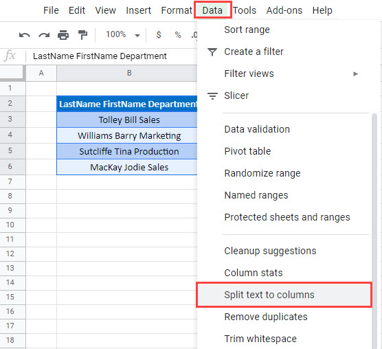
Click on Detect Automatically
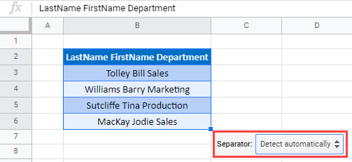
Select the Space.
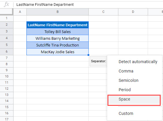
Your text will be split into columns.
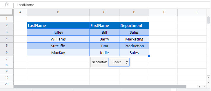
Split Text String by Comma or Other Character
You can use the FIND, LEFT, MID and RIGHT functions in Google Sheets as you do in Excel to split the text.
The formulas to extract the data for the LastName, FirstName and Department Columns are the same ones that are used in Excel.