
Excel for Microsoft 365 Excel for Microsoft 365 for Mac Excel for the web Excel 2021 Excel 2021 for Mac Excel 2019 Excel 2019 for Mac Excel 2016 Excel 2016 for Mac Excel 2013 Excel 2010 Excel 2007 Excel for Mac 2011 More…Less
Multiplying and dividing in Excel is easy, but you need to create a simple formula to do it. Just remember that all formulas in Excel begin with an equal sign (=), and you can use the formula bar to create them.
Multiply numbers
Let’s say you want to figure out how much bottled water that you need for a customer conference (total attendees × 4 days × 3 bottles per day) or the reimbursement travel cost for a business trip (total miles × 0.46). There are several ways to multiply numbers.
Multiply numbers in a cell
To do this task, use the * (asterisk) arithmetic operator.
For example, if you type =5*10 in a cell, the cell displays the result, 50.
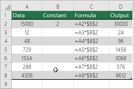
Multiply a column of numbers by a constant number
Suppose you want to multiply each cell in a column of seven numbers by a number that is contained in another cell. In this example, the number you want to multiply by is 3, contained in cell C2.
-
Type =A2*$B$2 in a new column in your spreadsheet (the above example uses column D). Be sure to include a $ symbol before B and before 2 in the formula, and press ENTER.
Note: Using $ symbols tells Excel that the reference to B2 is «absolute,» which means that when you copy the formula to another cell, the reference will always be to cell B2. If you didn’t use $ symbols in the formula and you dragged the formula down to cell B3, Excel would change the formula to =A3*C3, which wouldn’t work, because there is no value in B3.
-
Drag the formula down to the other cells in the column.
Note: In Excel 2016 for Windows, the cells are populated automatically.
Multiply numbers in different cells by using a formula
You can use the PRODUCT function to multiply numbers, cells, and ranges.
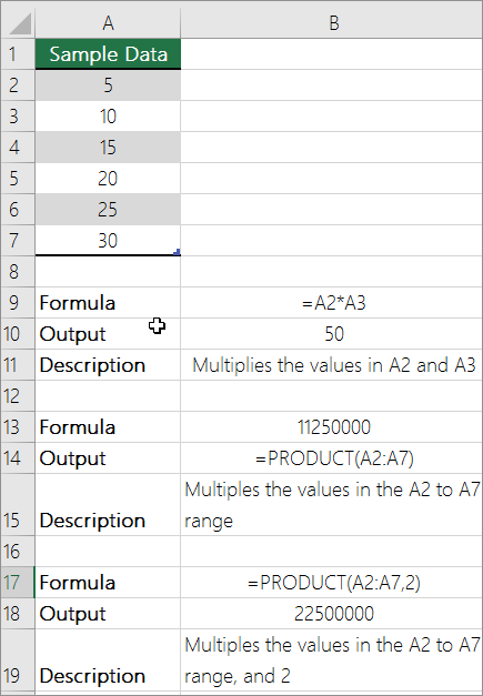
You can use any combination of up to 255 numbers or cell references in the PRODUCT function. For example, the formula =PRODUCT(A2,A4:A15,12,E3:E5,150,G4,H4:J6) multiplies two single cells (A2 and G4), two numbers (12 and 150), and three ranges (A4:A15, E3:E5, and H4:J6).
Divide numbers
Let’s say you want to find out how many person hours it took to finish a project (total project hours ÷ total people on project) or the actual miles per gallon rate for your recent cross-country trip (total miles ÷ total gallons). There are several ways to divide numbers.
Divide numbers in a cell
To do this task, use the / (forward slash) arithmetic operator.
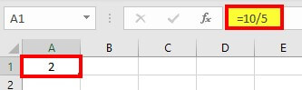
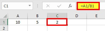
For example, if you type =10/5 in a cell, the cell displays 2.
Important: Be sure to type an equal sign (=) in the cell before you type the numbers and the / operator; otherwise, Excel will interpret what you type as a date. For example, if you type 7/30, Excel may display 30-Jul in the cell. Or, if you type 12/36, Excel will first convert that value to 12/1/1936 and display 1-Dec in the cell.
Note: There is no DIVIDE function in Excel.
Divide numbers by using cell references
Instead of typing numbers directly in a formula, you can use cell references, such as A2 and A3, to refer to the numbers that you want to divide and divide by.
Example:
The example may be easier to understand if you copy it to a blank worksheet.
How to copy an example
-
Create a blank workbook or worksheet.
-
Select the example in the Help topic.
Note: Do not select the row or column headers.

Selecting an example from Help
-
Press CTRL+C.
-
In the worksheet, select cell A1, and press CTRL+V.
-
To switch between viewing the results and viewing the formulas that return the results, press CTRL+` (grave accent), or on the Formulas tab, click the Show Formulas button.
|
A |
B |
C |
|
|
1 |
Data |
Formula |
Description (Result) |
|
2 |
15000 |
=A2/A3 |
Divides 15000 by 12 (1250) |
|
3 |
12 |
Divide a column of numbers by a constant number
Suppose you want to divide each cell in a column of seven numbers by a number that is contained in another cell. In this example, the number you want to divide by is 3, contained in cell C2.
|
A |
B |
C |
|
|
1 |
Data |
Formula |
Constant |
|
2 |
15000 |
=A2/$C$2 |
3 |
|
3 |
12 |
=A3/$C$2 |
|
|
4 |
48 |
=A4/$C$2 |
|
|
5 |
729 |
=A5/$C$2 |
|
|
6 |
1534 |
=A6/$C$2 |
|
|
7 |
288 |
=A7/$C$2 |
|
|
8 |
4306 |
=A8/$C$2 |
-
Type =A2/$C$2 in cell B2. Be sure to include a $ symbol before C and before 2 in the formula.
-
Drag the formula in B2 down to the other cells in column B.
Note: Using $ symbols tells Excel that the reference to C2 is «absolute,» which means that when you copy the formula to another cell, the reference will always be to cell C2. If you didn’t use $ symbols in the formula and you dragged the formula down to cell B3, Excel would change the formula to =A3/C3, which wouldn’t work, because there is no value in C3.
Need more help?
You can always ask an expert in the Excel Tech Community or get support in the Answers community.
See Also
Multiply a column of numbers by the same number
Multiply by a percentage
Create a multiplication table
Calculation operators and order of operations
Need more help?
There’s no DIVIDE function in Excel. Simply use the forward slash (/) to divide numbers in Excel.
1. The formula below divides numbers in a cell. Use the forward slash (/) as the division operator. Don’t forget, always start a formula with an equal sign (=).

2. The formula below divides the value in cell A1 by the value in cell B1.

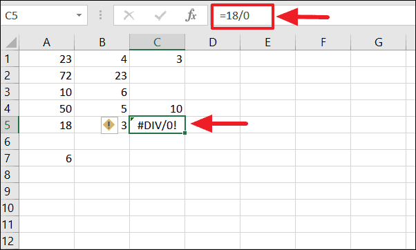
3. Excel displays the #DIV/0! error when a formula tries to divide a number by 0 or an empty cell.

4. The formula below divides 43 by 8. Nothing special.

5. You can use the QUOTIENT function in Excel to return the integer portion of a division. This function discards the remainder of a division.

6. The MOD function in Excel returns the remainder of a division.

Take a look at the screenshot below. To divide the numbers in one column by the numbers in another column, execute the following steps.
7a. First, divide the value in cell A1 by the value in cell B1.

7b. Next, select cell C1, click on the lower right corner of cell C1 and drag it down to cell C6.

Take a look at the screenshot below. To divide a column of numbers by a constant number, execute the following steps.
8a. First, divide the value in cell A1 by the value in cell A8. Fix the reference to cell A8 by placing a $ symbol in front of the column letter and row number ($A$8).

8b. Next, select cell B1, click on the lower right corner of cell B1 and drag it down to cell B6.

Explanation: when we drag the formula down, the absolute reference ($A$8) stays the same, while the relative reference (A1) changes to A2, A3, A4, etc.
If you’re not a formula hero, use Paste Special to divide in Excel without using formulas!
9. For example, select cell C1.

10. Right click, and then click Copy (or press CTRL + c).
11. Select the range A1:A6.
12. Right click, and then click Paste Special.
13. Click Divide.

14. Click OK.

Note: to divide numbers in one column by numbers in another column, at step 9, simply select a range instead of a cell.
Introduction to Divide in Excel
In Excel, the division is an arithmetic operation commonly used to divide numbers or values of the cell. It is one of the basic mathematical functions essential for solving complex numeric problems. Unlike addition, which has built-in functions such as the SUM function, no such function is available for division in Excel. To divide numbers or values of a cell in Excel, you need to start with an equal sign (=), followed by the numbers you want to divide, and put a forward slash (/) between the numbers.
Businesses often use the divide formula in Excel to calculate and perform various financial and work management tasks. For instance, they might calculate profit margins, monthly budgets, employee wages, expenditure reports, and other important metrics.
Let’s start by understanding how you can perform division in Excel.
Divide Formula in Excel
The arithmetic operation or formula for division in Excel starts with an equal sign (=) followed by entering the values or cell references you want to divide and a forward slash (/) between them.
![]()
How to Divide Numbers in a Cell in Excel?
To divide numbers in a cell, directly type the numbers within the cell and apply the divide formula. For example, if you want to divide 10 by 5, enter “=10/5” in a cell and press “Enter”. The division formula “=10/5” will give a result of 2.
Note: Please start the formula with an equal sign (=) and use the (/) operator between two values in each cell to get the output. Or else Excel will consider the equation as a date. For instance, If you only type 10/5 in a cell, Excel will display 05-Oct.
Example #1
You can download this Divide Formula Excel Template here – Divide Formula Excel Template
How to Divide Numbers Using Cell References?
You can divide the numbers of two cells by specifying the cell references in the divide formula.
For example, we want to divide the Cell A1 value by the Cell B1 value and display the result in Cell C1.
Solution:
Enter the formula “=A1/B1” in Cell C1 and press “Enter”, where the Cell A1 value is the dividend and Cell B2 value is the divisor. The result will be displayed in Cell C1.
Example #2
How to Divide a Column of Numbers by a Constant Number?
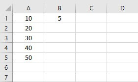
Suppose you want to divide the value of each cell of a column by a certain number obtained in another cell. You can easily do this task. In the below example, you will learn how to divide the values of column A by the value of Cell B1.
Solution:
Step 1: Click on Cell C1
Step 2: Enter the formula =”A1/$B$1” and press “Enter”.
Note: The symbol $ in Excel is used for absolute cell references. If you place a dollar sign ($) in front of a row, that row is fixed, and if you place a dollar sign ($) in front of a column, that column is fixed. In the formula =”A1/$B$1”, the value of the divisor is constant as the value of Cell B1.
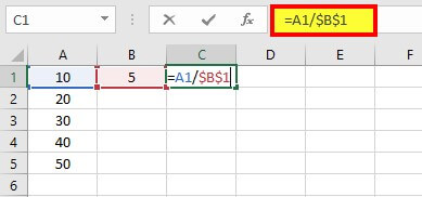
Result 2 is displayed in cell C1.
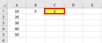
Step 3: Now, drag the cell with the formula to get the desired output.
Congratulations, you have successfully done this task.
Example #3
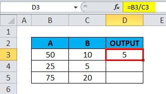
How to Divide Columns in Excel?
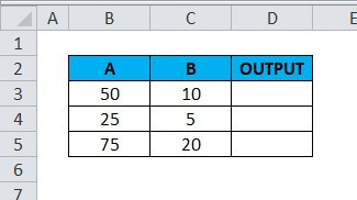
You can divide column 1 with column 2 by using the division formula. Consider the below table with numbers in columns A and B. Follow the below steps to learn how to divide two columns in Excel.
Solution:
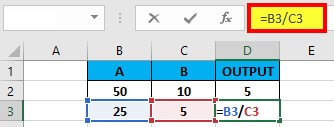
Step 1: Click on the Cell D3.
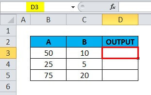
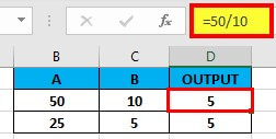
Step 2: Enter the formula “=B3/C3” in Cell D3, as shown below.
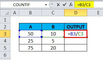
Result 5 is displayed in Cell D3.
Step 3: Drag the formula on the corresponding cell to get the following output.
Example #4
How to Use the Division (/) Operator with Subtraction Operators (-) in Excel?
Under this method, you will learn to use division operators with other arithmetic operators like subtraction to solve complex division problems.
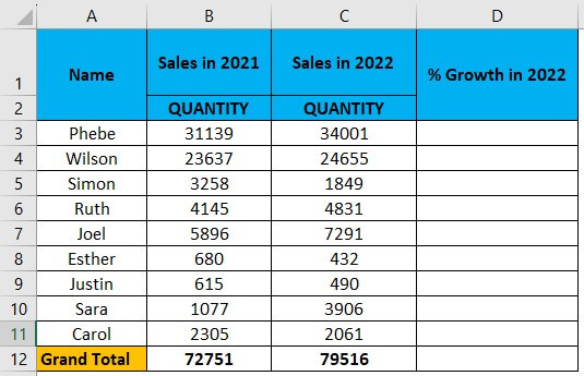
For example, you have the below data of salespersons and their actual sales in 2021 and 2022. You have to calculate the sales growth percentage for the respective salesperson in 2022. Here, you have to use the division formula along with the subtraction and percentage operator.
Solution:
Step 1: Click on the Cell D3
Step 2: Enter the formula “=(C3-B3)/B3” in Cell D3
Note: Using this formula, “=(C3-B3)/B3”, you can calculate the sales growth percentage for the respective salesperson.
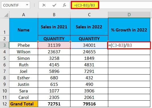
The output is 9%.
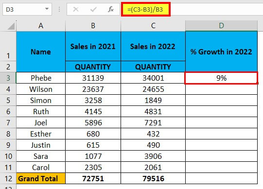
Note: The answer to the formula “=(C3-B3)/B3” is 0.091910466. For converting the decimal value into a percentage, select Cell D3, go to the “Home” tab, and click “Percentage” in the Number section. The result is 9%, as shown in the above image.
Step 3: Drag the cell with the formula downwards to get the desired output
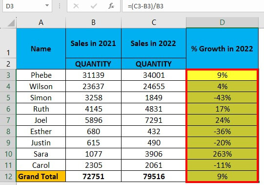
The above result shows the sales growth percentage for the individual salesperson.
Example # 5
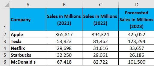
We have the sales data for five famous companies (Apple, Tesla, Netflix, Starbucks, and McDonald’s) for 2021 and 2022 and the estimated figures for 2023. We need to calculate the percentage growth rate for each company for 2023 using basic mathematical operators such as division, subtraction, and the percentage operator.
Solution:
Step 1: Add the title “% Growth in 2023” to column E, as shown below.
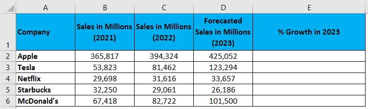
Step 2: Click on Cell E2.
Step 3: Enter the formula “=(D2-C2)/C2”, as shown below.
According to this formula, we will subtract the sales value of 2022 from 2023 and then divide the result by the sales value of 2022. The output is the percentage increase in sales from 2022 to 2023.
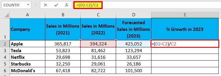
Note: In this example, we used the formula’s opening and closing parenthesis, “( )”.
The output is 8%, as shown below.
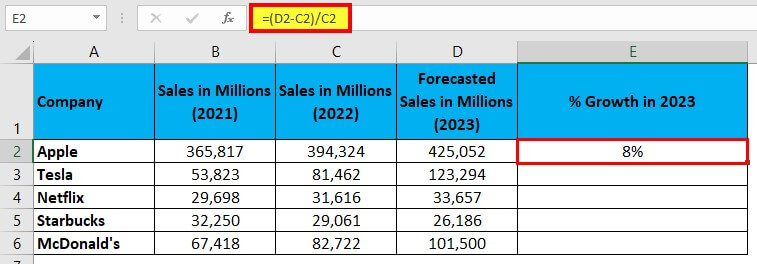
Note: The formula “=(B2+C2)/D2” will give a decimal value. Thus, convert this decimal value into %.
Step 4: Now, drag the cell with the formula to get the result, as shown below.
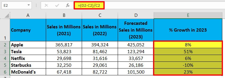
The future sales growth in percentage for all five companies in 2023 is now ready.
How to Use the Division Operator (/) with Addition (+)?
Under this method, you will learn to use the division operator with the addition operator (+) with the help of the following examples.
Example #6
Using Nested Parentheses in Division Operator Using Addition (+)
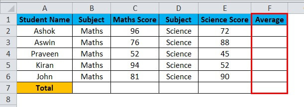
In this example, we will calculate the average of the student’s marks in maths and science by using the division and addition operator.
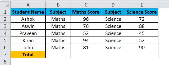
The formula for calculating the average marks of students is:“Total Number of Marks Scored / Number of Subjects.
Solution:
Step 1: Add a new column, “Average”, as shown below.
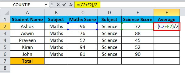
Step 2: Enter the formula “=(C2+E2)/2” in Cell F2.
The formula states to add the marks of Maths and Science subjects and then divide by the total subject, i.e., 2.
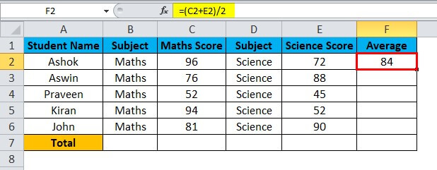
Result 84 is displayed, as shown in the below image.
Step 3: Now, drag the cell with the formula to the rest of the cells.
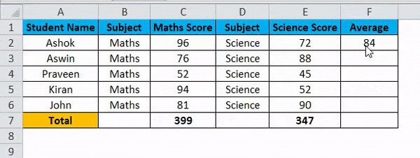
The average score of the students in Maths and Science subjects is displayed.
How to Handle #DIV/0! Error Using IF Function?
While executing the division operation on a data set, Excel will display the error of #DIV/0! when the formula tries to divide a number by an empty cell or 0. In the following example, you will learn how to use the IF function, such as the “IFERROR” condition, to prevent and resolve the #DIV/0! Error.
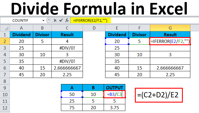
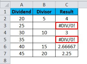
Suppose you have the below table of dividends and divisors. You have applied the division formula to this data, and Excel has shown error #DIV/0! in Cell C3 and Cell C5 because Cell B3 and Cell B5 have no value. Now, you want to overcome this problem.
Solution:
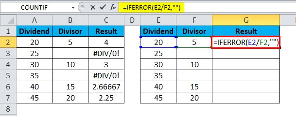
Step 1: Click Cell G2 of the Result column.
Step 2: Enter the IFERROR formula “=IFERROR(E2/F2,””)” as shown below and press “Enter”.
Note: The Formula “=IFERROR(E2/F2,””)” indicates that divide the value of Cell E2 by Cell F2, and if there is an empty cell or 0 value, then leave the cell blank in the result column to avoid displaying of the #DIV/0! Error.
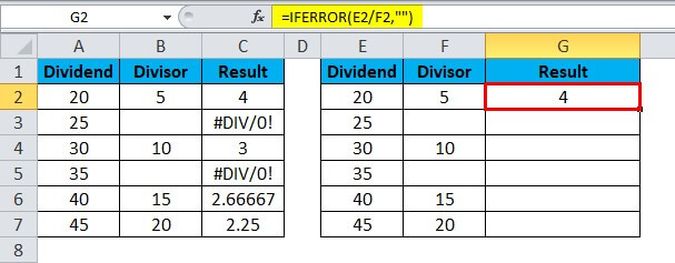
Output 4 is displayed.
Step 3: Drag the cell with the formula as shown below.
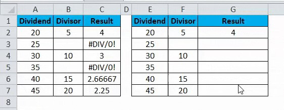
The result is displayed above, and Cell G3 and Cell G5 are blank instead of #DIV/0! Error.
Things to Remember while Using the Divide Function in Excel
- Put an equal sign (=) in the cell before using the divide formula.
- While selecting the data for calculation, do not select the row or column headers.
- If there is an empty cell or 0 value in the Cell, then Excel will throw an #DIV/0!
- You should properly use the opening and closing parenthesis in the division formula. For example, formulas like “=10/4-2” will give 0.5 output, and “=10/(4-2)” will give 5 output. Always remember, the “PEDMAS” is the order of calculations in Excel.
- If you want to display only the integer value of a division operation, use the QUOTIENT function of Excel.
Frequently Asked Questions (FAQS)
Q1. What is the symbol for the divide in Excel?
Answer: The symbol or arithmetic operator used to represent divide or division in Microsoft Excel is “/”, a forward slash. The Excel division formula is “=x/y,” where x is the dividend and y is the divisor.
Q2. How to divide in Excel?
Answer: There are various methods to divide in Excel. You can directly type the numbers in a cell or divide two (or more) numbers by referring to a cell or constant number. As seen in the image below, you must use an equal sign (=) before the division formula and a forward slash (/) between the numbers or cells you want to divide.
Q3. What is the other method for division in Excel?
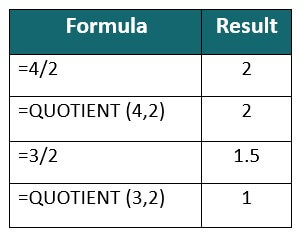
Answer: The alternate method for dividing numbers is using the “QUOTIENT” formula. When you want to display only the integer part of a division, use the formula “QUOTIENT(numerator, denominator)”. If a division equation has a remainder value, the QUOTIENT function will only return the integer value as an output. For example,” =3/2” returns 1.5 whereas “=QUOTIENT(3,2)” returns 1, where 1.5 is the remainder, and 1 is the integer/quotient.
Recommended Articles
This article has been a guide to Dividing in Excel. Here we discuss the Divide Formula in Excel and How to use Divide Formula in various scenarios using practical examples. You also get a downloadable Excel template for your reference. Furthermore, you can read our other suggested articles.
- Divide Cell in Excel
- Formatting Text in Excel
- Statistics in Excel
- Carriage Return in Excel
The Excel Formula for Division helps us perform the mathematical division between two numbers, i.e., one is the numerator and the other the denominator.
Excel doesn’t have an inbuilt Division formula. Therefore, we can use the basic method of using the equal “=” sign, and the arithmetic division operator, the forward slash “/”, to divide the values.
Table of Contents
- What Is Excel Formula For Division?
- How To Divide Using Excel Formulas?
- Basic Formula
- Examples
- How To Handle #DIV/0! Error In Excel Divide Formula?
- Important Things To Note
- Frequently Asked Questions
- Download Template
- Recommended Articles
- The Excel Formula for Division helps us divide 2 numeric values.
- We can use the Basic Division method using the arithmetic operator, i.e., by inserting the forward slash “/” in-between the 2 numeric values.
- We have the alternate division method, i.e., the QUOTIENT function, where both the arguments are mandatory and are not non-numeric.
- In case of a “#DIV/0!” error, we must use the IFERROR function to remove the error and replace it with any value according to our wish.
How To Divide Using Excel Formulas?
We can Divide Using Excel Formulas in 2 ways, namely,
- Basic Division Excel formula.
- Quotient Excel formula.
Method #1 – Basic Division Excel Formula
- First, type “=” in an empty cell.
- Next, for Value1, enter the first value or the cell reference holding the value, i.e., the numerator.
- Then, enter the “/” forward slash, i.e., the basic division symbol in Excel.
- Next, for Value2, enter the second value or the cell reference holding the value, i.e., the denominator.
- Finally, press the “Enter” key to execute the formula, and return the calculated result.
Therefore, the Basic Division Excel formula will be “=Value1/Value2”.
Method #2 – QUOTIENT Excel Formula
The syntax of the QUOTIENT Excel formula is,
The mandatory arguments of the QUOTIENT Excel formula are,
- Numerator: It is the number we are dividing.
- Denominator: It is the numeric value that we are dividing the numerator in excel.
The steps to use the QUOTIENT formula is,
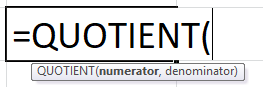
- First, type “=QUOTIENT(” in an empty cell.
- Next, enter the numerator and denominator values as numeric values or cell references.
- Finally, close the brackets and press the “Enter” key to execute the formula.
Basic Formula
Let us consider an example to use the Excel Formula for Division to divide numbers and calculate the percentages.
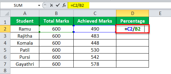
We have data of class students who recently appeared in the annual exam. We have the name and total marks they wrote for the exam and the total marks they obtained in the exam.
| Student | Total Marks | Achieved Marks | Percentage |
|---|---|---|---|
| Ramu | 600 | 490 | ? |
| Rajitha | 600 | 483 | ? |
| Komala | 600 | 448 | ? |
| Patil | 600 | 530 | ? |
| Pursi | 600 | 542 | ? |
| Gayathri | 600 | 578 | ? |
The steps to find the percentage of students are:
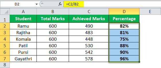
Step 1: Selectcell D2, and enter the formula =C2/B2, i.e., (Achieved Marks / Total Marks).
Step 2: Press the “Enter” key, and drag the formula from cell D2 to D7 using the fill handle. The output, i.e., the percentage of the students, is shown below.
Examples
We will consider a couple of examples using the QUOTIENT Excel Formula for Division.
Example #1
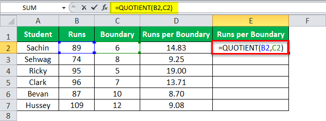
We have a cricket scorecard. The individual runs they scored and total boundaries they hit in their innings. We need to find how many runs once they score a boundary. We need to find how many runs once they score a boundary.
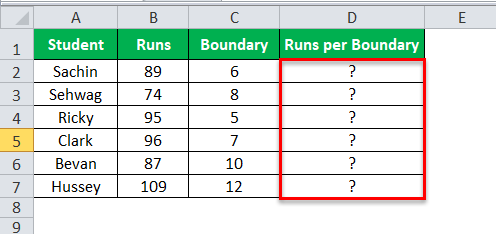
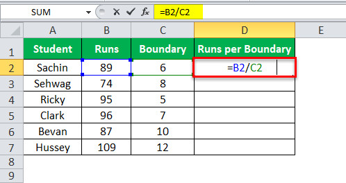
The steps to calculate using the QUOTIENT formula are,
Step 1: Select cell D2, enter the formula =B2/C2, press “Enter”, and drag the formula from cell D2 to D7 using the fill handle.

Step 2: Select cell E2, andenter the formula =QUOTIENT(B2,C2).
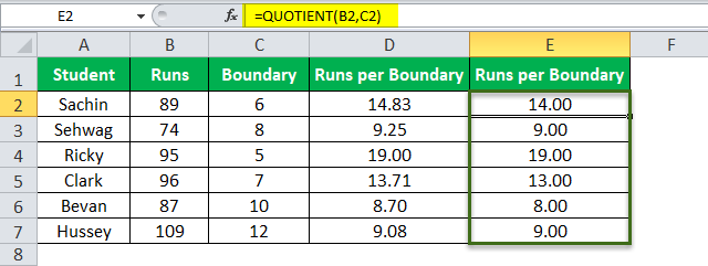
Step 3: Press the “Enter” key, and drag the formula from cell E2 to E7 using the fill handle.
[Note: The QUOTIENT function rounds down the values. However, it will not show the decimal values.]
The output is shown below, i.e., Sachin hits a boundary for every 14th run, Sehwag hits a boundary for every 9th run, etc.
Example #2
Let us consider a scenario of a unique problem.
One day I was busy with my analysis work, and one of the sales managers called and asked if I had an online client. I pitched him for $400,000 plus taxes, but he is asking me to include the tax in the $400,000 itself, i.e., he is requesting the product for $400,000 inclusive of taxes.
We need tax percentage, multiplication rule, and division rule to find the base value.
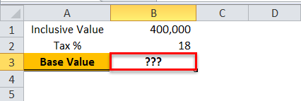
We must apply the Excel formula below to divide what we have shown in the image.
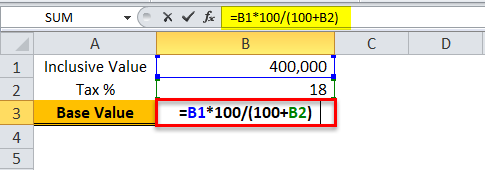
Firstly, the inclusive value is multiplied by 100, and then it is divided by 100 + tax percentage. So, that would give us the base value.
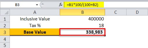
To cross-check, we can take 18% of $338,983, and add a percentage value of $338,983. We should get $400,000 as the overall value.
Sales managers can mention on the contract $338,983 + 18% tax.
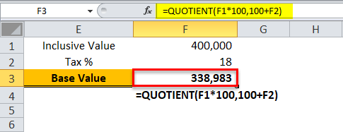
We can also do this by using the QUOTIENT function. The below image is an illustration of the same.
How To Handle #DIV/0! Error In Excel Divide Formula?
In excel, when we are dividing, we get excel errorsErrors in excel are common and often occur at times of applying formulas. The list of nine most common excel errors are — #DIV/0, #N/A, #NAME?, #NULL!, #NUM!, #REF!, #VALUE!, #####, Circular Reference.read more as “#DIV/0!”. This section of the article will explain how to deal with those errors.
We have a five years budget vs. the actual number. So, we need to find out the variance percentages.

The steps to apply the Excel formula to divide are,
Step 1: Select cell D2, and enter the formula =(B2-C2)/B2.
By deducting the actual cost from the budgeted cost, we get the “Variance Amount”, and then we will divide the “Variance Amount” by the “Budgeted Cost” to get the “Variance Percentage”.

Step 2: Press “Enter”, and drag the formula from cell D2 to D6 using the fill handle. The output is shown below.

Step 3: The problem here is we got an error in the last year, 2018, i.e., cell D6. Since there are no budgeted numbers in 2018, we got #DIV/0! error because we cannot divide any number by zero.
We can eliminate this error by using the IFERROR function in excelThe IFERROR function in Excel checks a formula (or a cell) for errors and returns a specified value in place of the error.read more.
Therefore, select cell D6, enter the formula =IFERROR((B6-C6)/B6,0), and press “Enter”.

The output is shown below. The IFERROR function in Excel converts all the error values to zero.
Important Things To Note
- We get the “#DIV/0!” error if the denominator is zero.
- We get the “#VALUE!” errorif the numerator/denominator or both the values are non-numeric.
- If we type the backward slash “” instead of the forward slash “/”, we get the “#NAME?” error.
- For the QUOTIENT function, both the arguments are mandatory.
Frequently Asked Questions
1) Does Excel have a Division formula?
Excel doesn’t have an inbuilt Division formula. Therefore, we can use the Basic Division Method by using the equal “=” sign, and the forward slash “/” sign to divide the numeric values.
The Basic Division Excel formula will be “=Value1/Value2”.
a) First, type “=” in an empty cell.
b) Next, for Value1, enter the first value or the cell reference holding the value, i.e., the numerator.
c) Then, enter the “/” forward slash, i.e., the basic division symbol in Excel.
d) Next, for Value2, enter the second value or the cell reference holding the value, i.e., the denominator.
e) Finally, press the “Enter” key to execute the formula, and return the calculated result.
2) What is an alternative method for division in Excel?
The alternate method to divide 2 numbers is by using the QUOTIENT formula as follows:
1) First, type “=QUOTIENT(” in an empty cell.
2) Next, enter the numerator and denominator values as numeric values or cell references.
3) Finally, close the brackets and press the “Enter” key to execute the formula.
3) Why is the Division Excel formula not working?
The Division Excel formula may not work for the following reasons,
• If one of the cell values is blank or empty.
• If the values are non-numeric.
• If the denominator is zero.
Download Template
This article must help understand Excel Formula For Division. Here we divide numbers using forward slash “/” operator & QUOTIENT(), examples & a downloadable template. You can download the template here to use it instantly.
You can download this Division Formula Excel Template here – Division Formula Excel Template
Recommended Articles
This article has been a step-by-step guide to Excel Formula For Division Here we discuss how to divide in Excel using the QUOTIENT function and handle #DIV/0! Error, along with practical examples and downloadable templates. You may learn more about Excel from the following articles: –
- Multiply in Excel Formula
- Excel Subtraction Formula
- Matrix Multiplication in Excel
- Percent Error Formula
How to Divide in Excel Using a Formula
Division formulas, #DIV/O! formula errors, and calculating percentages
Updated on February 2, 2021
What to Know
- Always begin any formula with an equal sign ( = ).
- For division, use the forward slash ( / )
- After entering in a formula, press Enter to complete the process.
This article explains how to divide in Excel using a formula. Instructions apply to Excel 2016, 2013, 2010, Excel for Mac, Excel for Android, and Excel Online.
Here are some important points to remember about Excel formulas:
- Formulas begin with the equal sign ( = ).
- The equal sign goes in the cell where you want the answer to display.
- The division symbol is the forward slash ( / ).
- The formula is completed by pressing the Enter key on the keyboard.
Use Cell References in Formulas
Although it is possible to enter numbers directly into a formula, it’s better to enter the data into worksheet cells and then use cell references as demonstrated in the example below. That way, if it becomes necessary to change the data, it is a simple matter of replacing the data in the cells rather than rewriting the formula. Normally, the results of the formula will update automatically once the data changes.
Example Division Formula Example
Let’s create a formula in cell B2 that divides the data in cell A2 by the data in A3.
The finished formula in cell B2 will be:
Enter the Data
-
Type the number 20 in cell A2 and press the Enter key.
To enter cell data in Excel for Android, tap the green check mark to the right of the text field or tap another cell.
-
Type the number 10 in cell A3 and press Enter.
Enter the Formula Using Pointing
Although it is possible to type the formula (=A2/A3) into cell B2 and have the correct answer display in that cell, it’s preferable to use pointing to add the cell references to formulas. Pointing minimizes potential errors created by typing in the wrong cell reference. Pointing simply means selecting the cell containing the data with the mouse pointer (or your finger if you’re using Excel for Android) to add cell references to a formula.
To enter the formula:
-
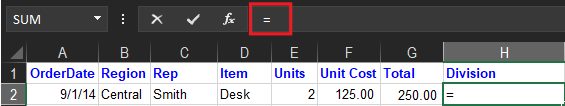
Type an equal sign ( = ) in cell B2 to begin the formula.
-
Select cell A2 to add that cell reference to the formula after the equal sign.
-
Type the division sign ( / ) in cell B2 after the cell reference.
-
Select cell A3 to add that cell reference to the formula after the division sign.
-
Press Enter (in Excel for Android, select the green check mark beside the formula bar) to complete the formula.
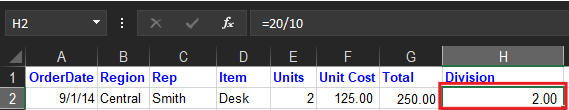
The answer (2) appears in cell B2 (20 divided by 10 is equal to 2). Even though the answer is seen in cell B2, selecting that cell displays the formula =A2/A3 in the formula bar above the worksheet.
Change the Formula Data
To test the value of using cell references in a formula, change the number in cell A3 from 10 to 5 and press Enter.
The answer in cell B2 automatically changes 4 to reflect the change in cell A3.
#DIV/O! Formula Errors
The most common error associated with division operations in Excel is the #DIV/O! error value. This error displays when the denominator in the division formula is equal to zero, which is not allowed in ordinary arithmetic. You may see this error if an incorrect cell reference was entered into a formula, or if a formula was copied to another location using the fill handle.
Calculate Percentages With Division Formulas
A percentage is a fraction or decimal that is calculated by dividing the numerator by the denominator and multiplying the result by 100. The general form of the equation is:
When the result, or quotient, of a division operation is less than one, Excel represents it as a decimal. That result can be represented as a percentage by changing the default formatting.
Create More Complex Formulas
To expand formulas to include additional operations such as multiplication, continue adding the correct mathematical operator followed by the cell reference containing the new data. Before mixing different mathematical operations together, it is important to understand the order of operations that Excel follows when evaluating a formula.
Thanks for letting us know!
Get the Latest Tech News Delivered Every Day
Subscribe
In Excel, you can divide in a cell, cells, columns of cells, a range of cells by a constant number, and by using the QUOTIENT function.

In Excel, you can divide within a cell, cell by cell, columns of cells, range of cells by a constant number, and divide using QUOTIENT function.
Dividing using Divide symbol in a cell
The easiest method to divide numbers in excel is by using the divide operator. In MS Excel, the divide operator is a forward slash (/).
To divide numbers in a cell, simply, start a formula with the ‘=’ sign in a cell, then enter the dividend, followed by a forward slash, followed by the divisor.
=number/numberFor example, to divide 23 by 4, you type this formula in a cell: =23/4
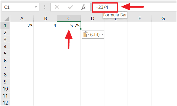
Dividing Cells in Excel
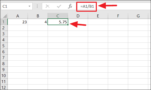
To divide two cells in Excel, enter the equals sign (=) in a cell, followed by two cell references with the division symbol in between. For example, to divide the cell value A1 by B1, type ‘=A1/B1’ in cell C1.
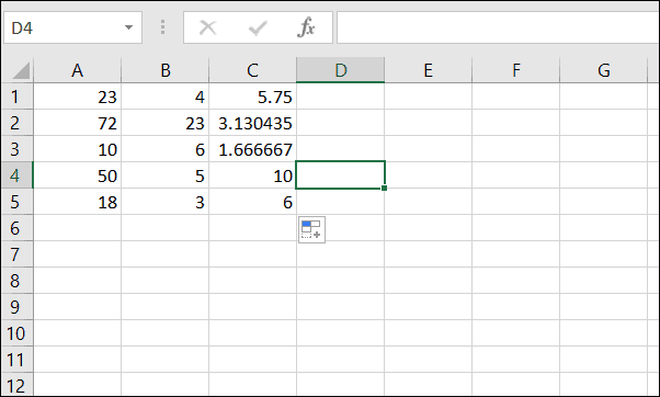
Dividing Columns of Cells in Excel
To divide two columns of numbers in Excel, you can use the same formula. After you, typed the formula in the first cell (C1 in our case), click on the small green square in the lower-right corner of cell C1 and drag it down to cell C5.
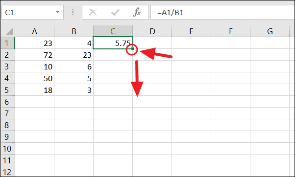
Now, the formula is copied from C1 to C5 of column C. And column A is divided by column B, and the answers were populated in column C.
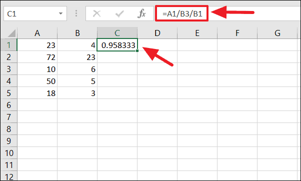
For example, to divide the number in A1 by the number in B2, and then divide the result by the number in B1, use the formula in the following image.
Dividing a Range of Cells by a Constant Number in Excel
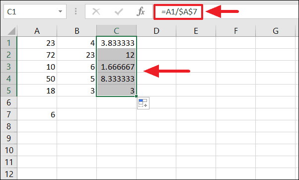
If you want to divide a range of cells in a column by a constant number, you can do that by fixing the reference to the cell that contains the constant number by adding the dollar ‘$’ symbol in front of the column and row in the cell reference. This way, you can lock that cell reference so it won’t change no matter where the formula is copied.
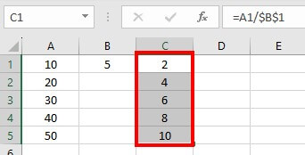
For example, we created an absolute cell reference by placing a $ symbol in front of the column letter and row number of cell A7 ($A$7). First, enter the formula in cell C1 to divide the value of cell A1 by the value of cell A7.
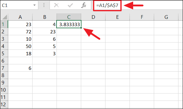
To divide a range of cells by a constant number, click on the small green square in the lower-right corner of cell C1 and drag it down to cell C5. Now, the formula is applied to C1:C5 and cell C7 is divided by a range of cells (A1:A5).
Divide a Column by the Constant Number with Paste Special
You can also divide a range of cells by the same number with Paste Special method. To do that, right-click on the cell A7 and copy (or press CTRL + c).
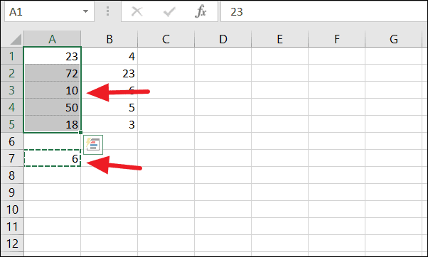
Next, select the cell range A1:A5 and then right-click, and click ‘Paste Special’.
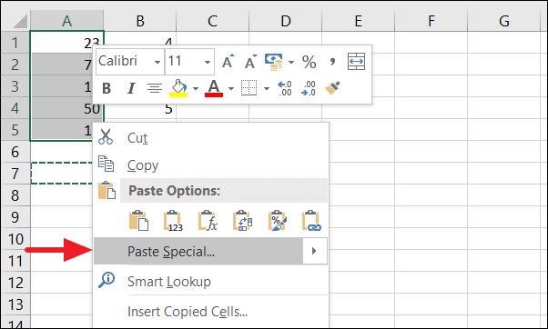
Select ‘Divide’ under ‘Operations’ and click the ‘OK’ button.
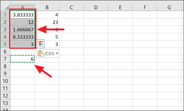
Now, cell A7 is divided by the column of numbers (A1:A5). But the original cell values of A1:A5 will be replaced with the results.
Dividing in Excel using QUOTIENT Function
Another way to divide in Excel is by using the QUOTIENT function. However, dividing numbers of cells using the QUOTIENT returns only the integer number of a division. This function discards the remainder of a division.
The Syntax for QUOTIENT function:
=QUOTIENT(numerator, denominator)When you divide two numbers evenly without remainder, the QUOTIENT function returns the same output as the division operator.
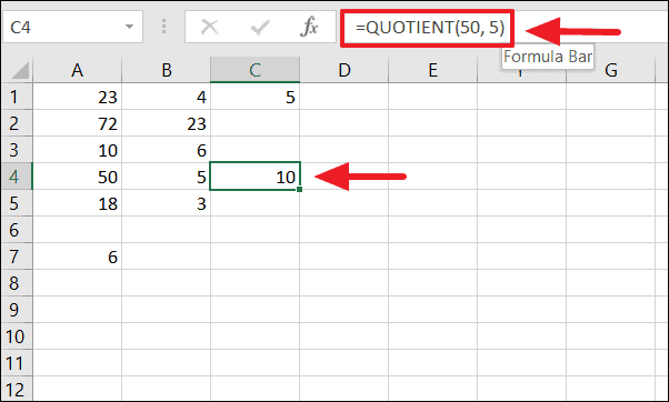
For example, both =50/5 and =QUOTIENT(50, 5) yields 10.
But, when you divide two numbers with a remainder, the divide symbol produces a decimal number while the QUOTIENT returns only the integer part of the number.
For example, =A1/B1 returns 5.75 and =QUOTIENT(A1,B1) returns 5.
If you only want the remainder of a division, not an integer, then use the Excel MOD function.
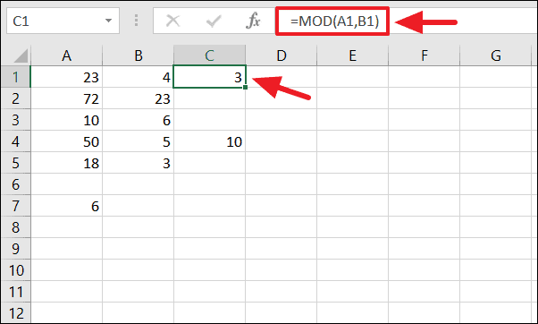
For example, =MOD(A1,B1) or =MOD(23/4) returns 3.
#DIV/O! Error
#DIV/O! error value is one of the most common errors associated with division operations in Excel. This error will be displayed when the denominator is 0 or the cell reference is incorrect.
We hope this post helps you divide in Excel.
Содержание
- Multiply and divide numbers in Excel
- Multiply numbers
- Multiply numbers in a cell
- Multiply a column of numbers by a constant number
- Multiply numbers in different cells by using a formula
- Divide numbers
- Divide numbers in a cell
- Divide numbers by using cell references
- Multiply and divide numbers in Excel
- Multiply numbers
- Multiply numbers in a cell
- Multiply a column of numbers by a constant number
- Multiply numbers in different cells by using a formula
- Divide numbers
- Divide numbers in a cell
- Divide numbers by using cell references
- Divide
- How to divide in Excel and handle #DIV/0! error
- Divide symbol in Excel
- How to divide numbers in Excel
- How to divide cell value in Excel
- Divide function in Excel (QUOTIENT)
- 3 things you should know about QUOTIENT function
- How to divide columns in Excel
- How to divide two columns in Excel by copying a formula
- How to divide one column by another with an array formula
- How to divide a column by a number in Excel
- Divide a column by number with a formula
- Divide a column by the same number with Paste Special
- How to divide by percentage in Excel
- Excel DIV/0 error
- Suppress #DIV/0 error with IFERROR
- Handle Excel DIV/0 error with IF formula
- How to divide with Ultimate Suite for Excel
Multiply and divide numbers in Excel
Multiplying and dividing in Excel is easy, but you need to create a simple formula to do it. Just remember that all formulas in Excel begin with an equal sign (=), and you can use the formula bar to create them.
Multiply numbers
Let’s say you want to figure out how much bottled water that you need for a customer conference (total attendees × 4 days × 3 bottles per day) or the reimbursement travel cost for a business trip (total miles × 0.46). There are several ways to multiply numbers.
Multiply numbers in a cell
To do this task, use the * (asterisk) arithmetic operator.
For example, if you type =5*10 in a cell, the cell displays the result, 50.
Multiply a column of numbers by a constant number
Suppose you want to multiply each cell in a column of seven numbers by a number that is contained in another cell. In this example, the number you want to multiply by is 3, contained in cell C2.
Type =A2*$B$2 in a new column in your spreadsheet (the above example uses column D). Be sure to include a $ symbol before B and before 2 in the formula, and press ENTER.
Note: Using $ symbols tells Excel that the reference to B2 is «absolute,» which means that when you copy the formula to another cell, the reference will always be to cell B2. If you didn’t use $ symbols in the formula and you dragged the formula down to cell B3, Excel would change the formula to =A3*C3, which wouldn’t work, because there is no value in B3.
Drag the formula down to the other cells in the column.
Note: In Excel 2016 for Windows, the cells are populated automatically.
Multiply numbers in different cells by using a formula
You can use the PRODUCT function to multiply numbers, cells, and ranges.
You can use any combination of up to 255 numbers or cell references in the PRODUCT function. For example, the formula =PRODUCT(A2,A4:A15,12,E3:E5,150,G4,H4:J6) multiplies two single cells (A2 and G4), two numbers (12 and 150), and three ranges (A4:A15, E3:E5, and H4:J6).
Divide numbers
Let’s say you want to find out how many person hours it took to finish a project (total project hours ÷ total people on project) or the actual miles per gallon rate for your recent cross-country trip (total miles ÷ total gallons). There are several ways to divide numbers.
Divide numbers in a cell
To do this task, use the / (forward slash) arithmetic operator.
For example, if you type =10/5 in a cell, the cell displays 2.
Important: Be sure to type an equal sign ( =) in the cell before you type the numbers and the / operator; otherwise, Excel will interpret what you type as a date. For example, if you type 7/30, Excel may display 30-Jul in the cell. Or, if you type 12/36, Excel will first convert that value to 12/1/1936 and display 1-Dec in the cell.
Note: There is no DIVIDE function in Excel.
Divide numbers by using cell references
Instead of typing numbers directly in a formula, you can use cell references, such as A2 and A3, to refer to the numbers that you want to divide and divide by.
The example may be easier to understand if you copy it to a blank worksheet.
How to copy an example
Create a blank workbook or worksheet.
Select the example in the Help topic.
Note: Do not select the row or column headers.

Selecting an example from Help
In the worksheet, select cell A1, and press CTRL+V.
To switch between viewing the results and viewing the formulas that return the results, press CTRL+` (grave accent), or on the Formulas tab, click the Show Formulas button.
Источник
Multiply and divide numbers in Excel
Multiplying and dividing in Excel is easy, but you need to create a simple formula to do it. Just remember that all formulas in Excel begin with an equal sign (=), and you can use the formula bar to create them.
Multiply numbers
Let’s say you want to figure out how much bottled water that you need for a customer conference (total attendees × 4 days × 3 bottles per day) or the reimbursement travel cost for a business trip (total miles × 0.46). There are several ways to multiply numbers.
Multiply numbers in a cell
To do this task, use the * (asterisk) arithmetic operator.
For example, if you type =5*10 in a cell, the cell displays the result, 50.
Multiply a column of numbers by a constant number
Suppose you want to multiply each cell in a column of seven numbers by a number that is contained in another cell. In this example, the number you want to multiply by is 3, contained in cell C2.
Type =A2*$B$2 in a new column in your spreadsheet (the above example uses column D). Be sure to include a $ symbol before B and before 2 in the formula, and press ENTER.
Note: Using $ symbols tells Excel that the reference to B2 is «absolute,» which means that when you copy the formula to another cell, the reference will always be to cell B2. If you didn’t use $ symbols in the formula and you dragged the formula down to cell B3, Excel would change the formula to =A3*C3, which wouldn’t work, because there is no value in B3.
Drag the formula down to the other cells in the column.
Note: In Excel 2016 for Windows, the cells are populated automatically.
Multiply numbers in different cells by using a formula
You can use the PRODUCT function to multiply numbers, cells, and ranges.
You can use any combination of up to 255 numbers or cell references in the PRODUCT function. For example, the formula =PRODUCT(A2,A4:A15,12,E3:E5,150,G4,H4:J6) multiplies two single cells (A2 and G4), two numbers (12 and 150), and three ranges (A4:A15, E3:E5, and H4:J6).
Divide numbers
Let’s say you want to find out how many person hours it took to finish a project (total project hours ÷ total people on project) or the actual miles per gallon rate for your recent cross-country trip (total miles ÷ total gallons). There are several ways to divide numbers.
Divide numbers in a cell
To do this task, use the / (forward slash) arithmetic operator.
For example, if you type =10/5 in a cell, the cell displays 2.
Important: Be sure to type an equal sign ( =) in the cell before you type the numbers and the / operator; otherwise, Excel will interpret what you type as a date. For example, if you type 7/30, Excel may display 30-Jul in the cell. Or, if you type 12/36, Excel will first convert that value to 12/1/1936 and display 1-Dec in the cell.
Note: There is no DIVIDE function in Excel.
Divide numbers by using cell references
Instead of typing numbers directly in a formula, you can use cell references, such as A2 and A3, to refer to the numbers that you want to divide and divide by.
The example may be easier to understand if you copy it to a blank worksheet.
How to copy an example
Create a blank workbook or worksheet.
Select the example in the Help topic.
Note: Do not select the row or column headers.
Selecting an example from Help
In the worksheet, select cell A1, and press CTRL+V.
To switch between viewing the results and viewing the formulas that return the results, press CTRL+` (grave accent), or on the Formulas tab, click the Show Formulas button.
Источник
Divide
There’s no DIVIDE function in Excel. Simply use the forward slash (/) to divide numbers in Excel.
1. The formula below divides numbers in a cell. Use the forward slash (/) as the division operator. Don’t forget, always start a formula with an equal sign (=).
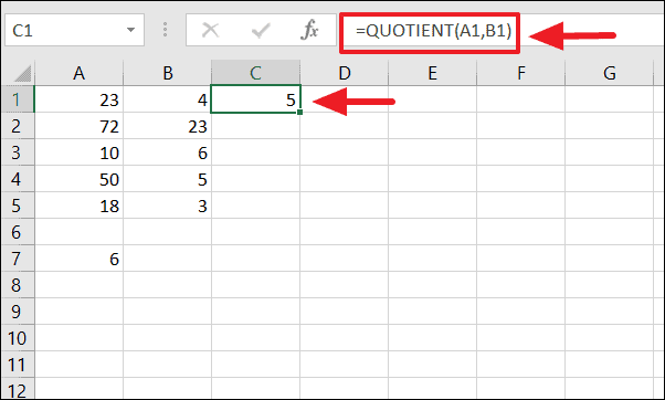
2. The formula below divides the value in cell A1 by the value in cell B1.
3. Excel displays the #DIV/0! error when a formula tries to divide a number by 0 or an empty cell.
4. The formula below divides 43 by 8. Nothing special.
5. You can use the QUOTIENT function in Excel to return the integer portion of a division. This function discards the remainder of a division.
6. The MOD function in Excel returns the remainder of a division.
Take a look at the screenshot below. To divide the numbers in one column by the numbers in another column, execute the following steps.
7a. First, divide the value in cell A1 by the value in cell B1.
7b. Next, select cell C1, click on the lower right corner of cell C1 and drag it down to cell C6.
Take a look at the screenshot below. To divide a column of numbers by a constant number, execute the following steps.
8a. First, divide the value in cell A1 by the value in cell A8. Fix the reference to cell A8 by placing a $ symbol in front of the column letter and row number ($A$8).
8b. Next, select cell B1, click on the lower right corner of cell B1 and drag it down to cell B6.
Explanation: when we drag the formula down, the absolute reference ($A$8) stays the same, while the relative reference (A1) changes to A2, A3, A4, etc.
If you’re not a formula hero, use Paste Special to divide in Excel without using formulas!
9. For example, select cell C1.
10. Right click, and then click Copy (or press CTRL + c).
11. Select the range A1:A6.
12. Right click, and then click Paste Special.
13. Click Divide.
Note: to divide numbers in one column by numbers in another column, at step 9, simply select a range instead of a cell.
Источник
How to divide in Excel and handle #DIV/0! error
 by Svetlana Cheusheva, updated on March 17, 2023
The tutorial shows how to use a division formula in Excel to divide numbers, cells or entire columns and how to handle Div/0 errors.
As with other basic math operations, Microsoft Excel provides several ways to divide numbers and cells. Which one to use depends on your personal preferences and a particular task you need to solve. In this tutorial, you will find some good examples of using a division formula in Excel that cover the most common scenarios.
Divide symbol in Excel
The common way to do division is by using the divide sign. In mathematics, the operation of division is represented by an obelus symbol (Г·). In Microsoft Excel, the divide symbol is a forward slash (/).
With this approach, you simply write an expression like =a/b with no spaces, where:
- a is the dividend — a number you want to divide, and
- b is the divisor — a number by which the dividend is to be divided.
How to divide numbers in Excel
To divide two numbers in Excel, you type the equals sign (=) in a cell, then type the number to be divided, followed by a forward slash, followed by the number to divide by, and press the Enter key to calculate the formula.
For example, to divide 10 by 5, you type the following expression in a cell: =10/5
The screenshot below shows a few more examples of a simple division formula in Excel: 
When a formula performs more than one arithmetic operation, it is important to remember about the order of calculations in Excel (PEMDAS): parentheses first, followed by exponentiation (raising to power), followed by multiplication or division whichever comes first, followed by addition or subtraction whichever comes first.
How to divide cell value in Excel
To divide cell values, you use the divide symbol exactly like shown in the above examples, but supply cell references instead of numbers.
- To divide a value in cell A2 by 5: =A2/5
- To divide cell A2 by cell B2: =A2/B2
- To divide multiple cells successively, type cell references separated by the division symbol. For example, to divide the number in A2 by the number in B2, and then divide the result by the number in C2, use this formula: =A2/B2/C2

Divide function in Excel (QUOTIENT)
I have to say plainly: there is no Divide function in Excel. Whenever you want to divide one number by another, use the division symbol as explained in the above examples.
However, if you want to return only the integer portion of a division and discard the remainder, then use the QUOTIENT function:
- Numerator (required) — the dividend, i.e. the number to be divided.
- Denominator (required) — the divisor, i.e. the number to divide by.
When two numbers divide evenly without remainder, the division symbol and a QUOTIENT formula return the same result. For example, both of the below formulars return 2.
When there is a remainder after division, the divide sign returns a decimal number and the QUOTIENT function returns only the integer part. For example:
=QUOTIENT(5,4) yields 1 
3 things you should know about QUOTIENT function
As simple as it seems, the Excel QUOTIENT function still has a few caveats you should be aware of:
- The numerator and denominator arguments should be supplied as numbers, references to cells containing numbers, or other functions that return numbers.
- If either argument is non-numeric, a QUOTIENT formula returns the #VALUE! error.
- If denominator is 0, QUOTIENT returns the divide by zero error (#DIV/0!).
How to divide columns in Excel
Dividing columns in Excel is also easy. It can done by copying a regular division formula down the column or by using an array formula. Why would one want to use an array formula for a trivial task like that? You will learn the reason in a moment 🙂
How to divide two columns in Excel by copying a formula
To divide columns in Excel, just do the following:
- Divide two cells in the topmost row, for example: =A2/B2
- Insert the formula in the first cell (say C2) and double-click the small green square in the lower-right corner of the cell to copy the formula down the column. Done!
Since we use relative cell references (without the $ sign), our division formula will change based on a relative position of a cell where it is copied: 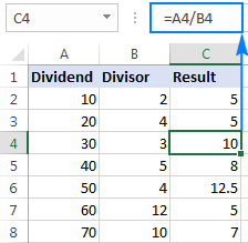
Tip. In a similar fashion, you can divide two rows in Excel. For example, to divide values in row 1 by values in row 2, you put =A1/A2 in cell A3, and then copy the formula rightwards to as many cells as necessary.
How to divide one column by another with an array formula
In situations when you want to prevent accidental deletion or alteration of a formula in individual cells, insert an array formula in an entire range.
For example, to divide the values in cells A2:A8 by the values in B2:B8 row-by-row, use this formula: =A2:A8/B2:B8
To insert the array formula correctly, perform these steps:
- Select the entire range where you want to enter the formula (C2:C8 in this example).
- Type the formula in the formula bar and press Ctrl + Shift + Enter to complete it. As soon as you do this, Excel will enclose the formula in , indicating it’s an array formula.
As the result, you will have the numbers in column A divided by the numbers in column B in one fell swoop. If someone tries to edit your formula in an individual cell, Excel will show a warning that part of an array cannot be changed.
To delete or modify the formula, you will need to select the whole range first, and then make the changes. To extend the formula to new rows, select the entire range including new rows, change the cell references in the formula bar to accommodate new cells, and then press Ctrl + Shift + Enter to update the formula. 
How to divide a column by a number in Excel
Depending on whether you want the output to be formulas or values, you can divide a column of numbers by a constant number by using a division formula or Paste Special feature.
Divide a column by number with a formula
As you already know, the fastest way to do division in Excel is by using the divide symbol. So, to divide each number in a given column by the same number, you put a usual division formula in the first cell, and then copy the formula down the column. That’s all there is to it!
For example, to divide values in column A by the number 5, insert the following formula in A2, and then copy it down to as many cells as you want: =A2/5 
As explained in the above example, the use of a relative cell reference (A2) ensures that the formula gets adjusted properly for each row. That is, the formula in B3 becomes =A3/5 , the formula in B4 becomes =A4/5 , and so on.
Instead of supplying the divisor directly in the formula, you can enter it in some cell, say D2, and divide by that cell. In this case, it’s important that you lock the cell reference with the dollar sign (like $D$2), making it an absolute reference because this reference should remain constant no matter where the formula is copied.
As shown in the screenshot below, the formula =A2/$D$2 returns exactly the same results as =A2/5 . 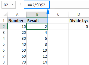
Divide a column by the same number with Paste Special
In case you want the results to be values, not formulas, you can do division in the usual way, and then replace formulas with values. Or, you can achieve the same result faster with the Paste Special > Divide option.
- If you don’t want to override the original numbers, copy them to the column where you want to have the results. In this example, we copy numbers from column A to column B.
- Put the divisor in some cell, say D2, like shown in the screenshot below.
- Select the divisor cell (D5), and press Ctrl + C to copy it to the clipboard.
- Select the cells you want to multiply (B2:B8).
- Press Ctrl + Alt + V , then I , which is the shortcut for Paste Special >Divide, and hit the Enter key.

Alternatively, right-click the selected numbers, select Paste Special… from the context menu, then select Divide under Operation, and click OK. 
Either way, each of the selected numbers in column A will be divided by the number in D5, and the results will be returned as values, not formulas: 
How to divide by percentage in Excel
Since percentages are parts of larger whole things, some people think that to calculate percentage of a given number you should divide that number by percent. But that is a common delusion! To find percentages, you should multiply, not divide. For example, to find 20% of 80, you multiply 80 by 20% and get 16 as the result: 80*20%=16 or 80*0.2=16.
In what situations do you divide a number by percentage? For instance, to find X if a certain percent of X is Y. To make things clearer, let’s solve this problem: 100 is 25% of what number?
To get the answer, convert the problem to this simple equation:
With Y equal to 100 and P to 25%, the formula takes the following shape: =100/25%
Since 25% is 25 parts of a hundred, you can safely replace the percentage with a decimal number: =100/0.25
As shown in the screenshot below, the result of both formulas is 400: 
For more examples of percentage formulas, please see How to calculate percentages in Excel.
Excel DIV/0 error
Division by zero is an operation for which there exists no answer, therefore it is disallowed. Whenever you try to divide a number by 0 or by an empty cell in Excel, you will get the divide by zero error (#DIV/0!). In some situations, that error indication might be useful, alerting you about possible faults in your data set.
In other scenarios, your formulas can just be waiting for input, so you may wish to replace Excel Div 0 error notations with empty cells or with your own message. That can be done by using either an IF formula or IFERROR function.
Suppress #DIV/0 error with IFERROR
The easiest way to handle the #DIV/0! error in Excel is to wrap your division formula in the IFERROR function like this:
The formula checks the result of the division, and if it evaluates to an error, returns an empty string («»), the result of the division otherwise.
Please have a look at the two worksheets below. Which one is more aesthetically pleasing? 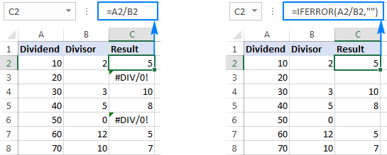
Note. Excel’s IFERROR function disguises not only #DIV/0! errors, but all other error types such as #N/A, #NAME?, #REF!, #VALUE!, etc. If you’d like to suppress specifically DIV/0 errors, then use an IF formula as shown in the next example.
Handle Excel DIV/0 error with IF formula
To mask only Div/0 errors in Excel, use an IF formula that checks if the divisor is equal (or not equal) to zero.
If the divisor is any number other than zero, the formulas divide cell A2 by B2. If B2 is 0 or blank, the formulas return nothing (empty string). 
Instead of an empty cell, you could also display a custom message like this:
=IF(B2<>0, A2/B2, «Error in calculation») 
How to divide with Ultimate Suite for Excel
If you are making your very first steps in Excel and do not feel comfortable with formulas yet, you can do division by using a mouse. All it takes is our Ultimate Suite installed in your Excel.
In one of the examples discussed earlier, we divided a column by a number with Excel’s Paste Special. That involved a lot of mouse movement and two shortcuts. Now, let me show you a shorter way to do the same.
- Copy the numbers you want to divide in the «Results» column to prevent the original numbers from being overridden.
- Select the copied values (C2:C5 in the screenshot below).
- Go to the Ablebits tools tab >Calculate group, and do the following:
- Select the divide sign (/) in the Operation box.
- Type the number to divide by in the Value box.
- Click the Calculate button.
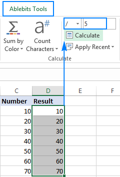
Done! The entire column is divided by the specified number in the blink of an eye: 
As with Excel Paste Special, the result of division is values, not formulas. So, you can safely move or copy the output to another location without worrying about updating formula references. You can even move or delete the original numbers, and your calculated numbers will be still safe and sound.
That is how you divide in Excel by using formulas or Calculate tools. If are curious to try this and many other useful features included with the Ultimate Suite for Excel, you are welcome to download 14-day trial version.
To have a closer look at the formulas discussed in this tutorial, feel free to download our sample workbook below. I thank you for reading and hope to see you on our blog next week!
Источник
This time we will venture how to divide division formulas in Excel; we will use examples, syntax, and figures to easy to understand and practice it your perspective.
Microsoft Excel provides different ways how to divide numbers and cells just like in any other basic math operator. It is in your hands what ways you will use considering your preference and requirements of your task. This is the continuation of our tutorial How To Multiply Cells In Excel With Examples.
Additionally, Microsoft Excel is a tool helpful in data entry, management of tasks, recording, and accounting stuff. Therefore a lot of business and work tasks use this application in organizing data and making financial analyses connecting to dividing a load task and finances.
Furthermore, if you use Excel thus encounter mathematical calculations such as division in your worksheet.
What is the Division Formula in Excel
Particularly, Excel does not have a division formula or function, but there are a lot of alternatives we can use. Along with this, you can use an arithmetic operation symbol (/) or a quotient function. Later we will know the things to remember in creating a formula but first, let’s know the syntax…
Syntax
=number1 / number2
It means that the =the number being divided / the number you are dividing by.
Divide symbol
In a division in Excel, the common way to execute it using the division sign. Thus, in arithmetic operations, the division operator uses the obelus symbol (÷) while in excel it uses a forward slash (/) symbol representing it.
Wherefore the expression of this process is written like this =a/b with no spaces where:
- a is the dividend – a number you want to divide, and
- b is the divisor – a number by which the dividend is to be divided.
So here are a few reminders to be kept in mind in creating a formula. This will help you while we jump specifically into dividing in Excel.
- First the equal sign(=). All the formulas must begin with this sign so that Excel will recognize them as formulas.
- Use cell reference. This is where the result of the formula is displayed, not the actual formula. Thus, helpful to enter the data in the cell and if you need to go back to later values, it will be easier to understand.
- Consider PEMDAS (Parenthesis, Exponentiation, Multiplication, Division, Addition, Subtraction) as a reference in the order of arithmetic operations. Below you’ll find an example of how the order of operations is applied to formulas in Excel.
Example 1: Using Numbers Directly
Here’s how to divide in Excel by typing numbers directly into the cell:
- Click the cell where you want the result displayed.
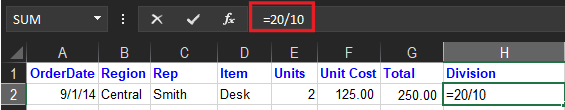
- Type the equal sign(=).
- Create your expression with the operator symbol (/). For instance, if you want to divide 20 by 10, enter 20/10 after the equal sign.
- When you press enter. In the example above, the result would be 2.
Note: Importantly, type equal sign (=) in the cell before you type, the number and the / operator otherwise Excel will read it as date.
For example, if you type 11/10, Excel may display 10-Nov in the cell. Or, if you type 10/20, Excel will first convert that value to 10/30/2020 and display 20-Oct in the cell.
Example 2: Using cell references
Here’s how to divide in Excel by using cell references instead of typing numbers directly into the cell:
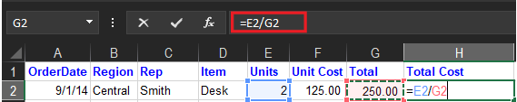
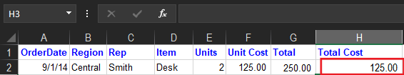
- Select the cell where you want the result to appear.
- Type the equal sign, and use cell references instead of typing regular numbers. For instance, if you want to divide cell E2 by cell G2, enter the formula =E2/G2.
- When you press enter key, Excel displays the result in the cell.
What is the QUOTIENT function in Excel?
The quotient Function is a formula where it divides the two numbers but returns the integer portion of a division. Moreover, it displays a whole number because it discards the rest. For instance, you want to have a quotient of 5 and 2 so the output is 2.5, hence it yields 2 only as the quotient only displays an integer.
How to use the QUOTIENT function in Excel
So here are the steps on how to use QUOTIENT FUNCTION in Excel:
- First, click the cell you want the result to display.
- Enter the =QUOTIENT() into the cell.
- After the parenthesis, type the first number, the dividend, followed by a comma. Then, enter the divisor which is the second number. Then, close the parenthesis.
- It divides numbers in excel when you press enter.
Apparently, the value in the first number or numerator and denominator or second number for a quotient function could be a number, reference cell, cell, or both.
Examples of these are:
- =QUOTIENT(5,2)
- =QUOTIENT(A4,16)
- =QUOTIENT(B2:C3)
Summary
In conclusion, learning how to divide in Excel is very helpful in complying with each task and requirement in business or on daily activities.
Thank you for reading!
Explanation
Learn how to divide numbers in Excel. After reading and practicing this tutorial, you will know how to calculate a value divided by another value.
Check out our Excel Basics tutorial where you can learn Excel’s fundamentals.
Scroll to the bottom of the page to practice division in Excel!
Example
If you want to divide numbers In Excel, use the sign Slash (/) sign. See the example below:

Learn how to divide numbers in Excel in two simple steps
Divide Values – Two steps formula
Step 1 – Always start a formula by using the = (equals) sign
Step 2 – Use the Slash(/) sign to divide values by each other
The formula should look like this:
= NUMBER / NUMBER
Let’s practice and learn how to divide numbers:
Important links
- Excel Basics