
Split text into different columns with the Convert Text to Columns Wizard
Take text in one or more cells and split it into multiple cells using the Convert Text to Columns Wizard.

Try it!
-
Select the cell or column that contains the text you want to split.
-
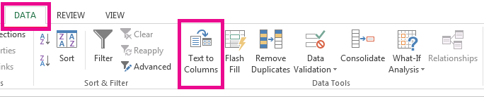
Select Data > Text to Columns.
-
In the Convert Text to Columns Wizard, select Delimited > Next.
-
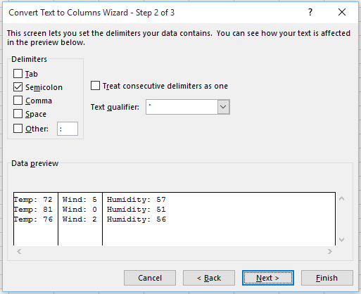
Select the Delimiters for your data. For example, Comma and Space. You can see a preview of your data in the Data preview window.
-
Select Next.
-
Select the Destination in your worksheet which is where you want the split data to appear.
-
Select Finish.
Want more?
Split text into different columns with functions
Need more help?
Bottom Line: Learn how to use formulas and functions in Excel to split full names into columns of first and last names.
Skill Level: Intermediate
Watch the Tutorial
Download the Excel Files
You can download both the before and after files below. The before file is so you can follow along, and the after file includes all of the formulas already written.
Splitting Text Into Separate Columns
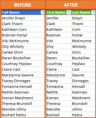
We’ve been talking about various ways to take the text that is in one column and divide it into two. Specifically, we’ve been looking at the common example of taking a Full Name column and splitting it into First Name and Last Name.
The first solution we looked at used Power Query and you can view that tutorial here: How to Split Cells and Text in Excel with Power Query. Then we explored how to use the Text to Columns feature that’s built into Excel: Split Cells with Text to Columns in Excel. Today, I want to show you how to accomplish the same thing with formulas.
Using 4 Functions to Build our Formulas
To split our Full Name column into First and Last using formulas, we need to use four different functions. We’ll be using SEARCH and LEFT to pull out the first name. Then we’ll use LEN and RIGHT to pull out the last name.
The SEARCH Function
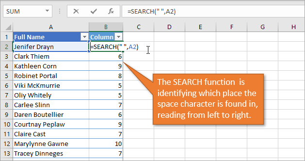
They key to breaking up the first names from the last names is for Excel to identify what all of the full names have in common. That common factor is the space character that separates the two names. To help our formula identify everything to the left of that space character as the first name, we need to use the SEARCH function.
The SEARCH function returns the number of the character at which a specific character or text string is found, reading left to right. In other words, what number is the space character in the line of characters that make up a full name? In my name, Jon Acampora, the space character is the 4th character (after J, o, and n), so the SEARCH function returns the number 4.
There are three arguments for SEARCH.
- The first argument for the SEARCH function is find_text. The text we want to find in our entries is the space character. So, for find_text, we enter ” “, being sure to include the quotation marks.
- The second argument is within_text. This is the text we are searching in for the space character. That would be the cell that has the full name. In our example, the first cell that has a full name is A2. Since we are working with Excel Tables, the formula will copy down and change to B2, C2, etc., for each respective row.
- The third and last argument is [start_num]. This argument is for cases where you want to ignore a certain number of characters in the text before beginning your search. In our case, we want to search the entire text, beginning with the very first character, so we do not need to define this argument.
All together, our formula reads: =SEARCH(” “,A2)
I started with the SEARCH function because it will be used as one of the arguments for the next function we’re going to look at. That is the LEFT function,
The LEFT Function
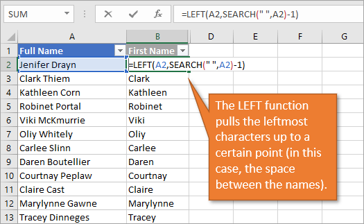
The LEFT function returns the specified number of characters from the start of a text string. To specify that number, we will use the value we just identified with the SEARCH function. The LEFT function will pull out the letters from the left of the Full Name column.
The LEFT function has two arguments.
- The first argument is text. That is just the cell that the function is pulling from—in our case A2.
- The second argument is [num_chars]. This is the number of characters that the function should pull. For this argument, we will use the formula we created above and subtract 1 from it, because we don’t want to actually include the space character in our results. So for our example, this argument would be SEARCH(” “,A2)-1
All together, our formula reads =LEFT(A2,SEARCH(” “,A2)-1)
Now that we’ve extracted the first name using the LEFT function, you can guess how we’re going to use the RIGHT function. It will pull out the last name. But before we go there, let me explain one of the components that we will need for that formula. That is the LEN function.
The LEN Function
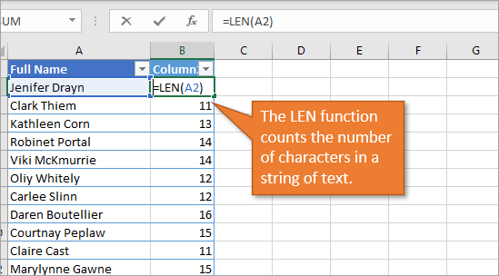
LEN stands for LENGTH. This function returns the number of characters in a text string. In my name, there are 12 characters: 3 for Jon, 8 for Acampora, and 1 for the space in between.
There is only one argument for LEN, and that is to identify which text to count characters from. For our example, we again are using A2 for the Full Name. Our formula is simply =LEN(A2)
The RIGHT Function
The RIGHT formula returns the specified number of characters from the end of a text string. RIGHT has two arguments.
- The first argument is text. This is the text that it is looking through in order to return the right characters. Just as with the LEFT function above, we are looking at cell A2.
- The second argument is [num_chars]. For this argument we want to subtract the number of characters that we identified using the SEARCH function from the total number of characters that we identified with the LEN function. That will give us the number of characters in the last name.
Our formula, all together, is =RIGHT(A2,LEN(A2)-SEARCH(” “,A2))
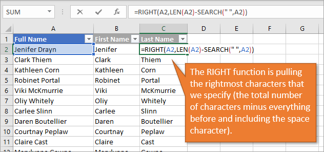
Note that we did not subtract 1 like we did before, because we want the space character included in the number that is being deducted from the total length.
Pros and Cons for Using Formulas to Split Cells
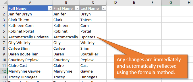
The one outstanding advantage to this method for splitting text is the automatic updates. When edits, additions, or deletions are made to the Full Name column, the First and Last names change as well. This is a big benefit compared to using Text to Columns, which requires you to completely repeat the process when changes are made. And even the Power Query method, though much simpler to update than Text to Columns, still requires a refresh to be manually selected.
Of course, one obvious disadvantage to this technique is that even though each of the four functions are relatively simple to understand, it takes some thought and time to combine them all and create formulas that work correctly. In other words, is not the easiest solution to implement of the three methods presented thus far.
Another disadvantage to consider is the fact that this only works for scenarios that have two names in the Full Name column. If you have data that includes middle names or two first names, the formula method isn’t helpful without making some considerable modifications to the formulas. (Homework challenge! If you’d like to give that a try, please do so and let us know your results in the comments.) As we saw in the Power Query tutorial, you do in fact have the capability to pull out more than two names with that technique.
Here are the links to the other posts on ways to split text:
- Split Cells with Text to Columns in Excel
- How to Split Text in Cells with Flash Fill in Excel
- How to Split Cells and Text in Excel with Power Query
- Split by Delimiter into Rows (and Columns) with Power Query
Conclusion
I hope you’ve learned something new from this post and that is helpful as you split data into separate columns. If you have questions or remarks, please leave a comment below!
One scenario is where you need to join multiple strings of text into a single text string. The flip of that is splitting a single text string into multiple text strings. If the data at hand was copied from somewhere or created by someone who completely missed the point of Excel columns, you will find that you need to split a block of text to categorize it.
Splitting the text largely depends on the delimiter in the text string. A delimiter is a character or symbol that marks the beginning or end of a character string. Examples of a delimiter are a space character, hyphen, period, comma.
 1")
Our example case for this guide involves splitting book details into book title, author, and genre. The delimiter we’ve used is a comma:
 2")
This tutorial will teach you how to split text in Excel with the Text to Columns and Flash Fill features, formulas, and VBA. The formulas method includes splitting text by a specific character. That’s the menu today.
Let’s get splitting!
Using Text to Columns
This feature lives up to its name. Text to Columns splits a column of text into multiple columns with specified controls. Text to Columns can split text with delimiters and since our data contains only a comma as the delimiter, using the feature becomes very easy. See the following steps to split text using Text to Columns:
- Select the data you want to split.
- Go to the Data tab and select the Text to Columns icon from the Data Tools
 3")
- Select the Delimited radio button and then click on the Next
 4")
- In the Delimiters section, select the Comma
- Then select the Next button.
 5")
- Now you need to choose where you want the split text. Click on the Destination field, then select the destination cell on the worksheet in the background where you want the split text to start.
- Select the Finish button to close the Text to Columns
 6")
Using the comma delimiter to separate the text string, Text to Columns has split the text from our example case into three columns:
 7")
Luckily, our data doesn’t contain a book with commas in the book name. If we had the book Cows, Pigs, Wars and Witches by Marvin Harris in the dataset, the text would be split into 5 columns instead of 3 like the rest. If the delimiter in your data is appearing in the text string for more than delimiting, you’ll have better luck splitting text with other methods. Now unto another observation.
Using TRIM Function to Trim Extra Spaces
Let’s cast a closer look at the output of Text to Columns. Notice how the last two columns carry one leading space? You can see that the values in columns D and E are not a hundred percent aligned to the left:
 8")
The last two columns carry a leading space because Text to Columns only takes the delimiter as a mark from where to split the text. The space character after the comma is carried with the next unit of text and that has our data with a leading space.
A quick fix for this is to use the TRIM function to clear up extra spaces. Here is the formula we have used to remove leading spaces from columns D and E:
=TRIM(C4)
The TRIM function removes all spaces from a text string other than a single space character between two words. Any leading, trailing, or extra spaces will be removed from the cell’s value. We have simply used the formula with a reference of the cell containing the leading space.
And that cleaned up the leading spaces for us. Data – good to go!
 9")
Using Formula To Separate Text in Excel
We can make use to Excel functions to construct formulas that can help us in splitting a text string into multiple.
Split String with Delimiter
Using a formula can also split a single text string into multiple strings but it will require a combo of functions. Let’s have a little briefing on the functions that make part of this formula we will use for splitting text.
The SUBSTITUTE function replaces old text in a text string with new text.
The REPT function repeats text a given number of times.
The LEN function returns the number of characters in a text string.
The MID function returns a given number of characters from the middle of a text string with a specified starting position.
The TRIM function removes all spaces, other than single spaces between words, from a text string.
Now let’s see how these functions combined can be used to split text with a single formula:
=TRIM(MID(SUBSTITUTE($B5,",",REPT(" ",LEN($B5))),(C$4-1)*LEN($B5)+1,LEN($B5)))
In our example, the first cell we are using this formula on is cell B5. The number of characters in B5 as counted by the LEN function is 49. The REPT function repeats spaces (denoted by “ “ in the formula) in B5 for the number of characters supplied by the LEN function i.e. 49.
The SUBSTITUTE function replaces the commas “,” in B5 with 49 space characters supplied by the REPT function. Since there are two commas in B5, one after the book name and one after the author, 49 spaces will be entered after the book name and 49 spaces after the author, creating a decent gap between the text we want to split.
Now let’s see the calculations for the MID function. The first bit is (C$4-1). In row 4, we added serial numbering for each of the columns for our categories. The row has been locked in the formula with a $ sign so the row doesn’t change as the formula is copied down. But we have left the column free so that the serial number changes for the respective columns used in the formula.
In the formula, 1 is subtracted from C4 (1-1=0) and the result is multiplied by the number of characters in B5 i.e. LEN($B5) and then 1 is added to the expression. The calculation for the starting position in the MID function, i.e. (C$4-1)*LEN($B5)+1, becomes (1-1)*49+1 which equals 1.
The MID function returns the text from the middle of B5, the starting position is 1 (that means the text to be returned is to start from the first character) and the number of characters to be returned is LEN($B5) i.e 49 characters. Since we have added 49 spaces in place of each of the commas, that gives us plenty of area to safely return just one chunk of text along with some extra spaces. The result up until the MID function is A Song of Ice and Fire with lots of trailing spaces.
The extra spaces are no problem. The TRIM function cleans any extra spaces leaving the single spaces between words and so we finally have the book name returned as A Song of Ice and Fire.
 10")
Now for the next column and hence the next category, the calculation for the starting position in the MID function will change like so (D$4-1)*LEN($B5)+1. The expression comes down to (2-1)*49+1 which equals 50. If the MID function is to return characters starting from the 50th character, with all the extra spaces added by the REPT function, what the MID function will return will be along this pattern: spaces author spaces.
The leading and trailing spaces will be trimmed by the TRIM function and the result will be George RR Martin.
 11")
The “+1” in the starting position argument of the MID function has no relevance for the subsequent columns, only for the first. That is because, without the “+1” in the first column’s calculation, it would be 0*49 which will end up in a #VALUE! error.
The formula copied along column E gives us the genre from the combined text in column B and that completes our set.
Split String at Specific Character
If there is only a single delimiter that is a specific character, such a lengthy formula as above will not be required to split the text. Let’s say, like our case example below, we are to split product code and product type which is joined by a hyphen.
Now this would be easier if the product code had a fixed number of characters; we would only have to use the LEFT function to return a certain number of characters. But what’s the fun in that?
We are going to let the FIND function do a bit of search work for us and find the hyphen in the text so the LEFT function and RIGHT function can return the surrounding text. This is the formula with the LEFT function for returning the first extract:
=LEFT(B3,FIND("-",B3)-1)
The FIND function searches B3 for the position of the hyphen “-“ in the text string, which is 6. The LEFT function then returns the characters starting from the left of the text and the number of characters to return is 6-1. “-1” at the end ensures that the characters returned do not include the hyphen itself. Here are the results of this formula for returning the first segment of split text:
 12")
Now for the second segment of text, the RIGHT function comes into play with this formula:
=RIGHT(B3,LEN(B3)-FIND("-",B3))
The FIND function is again used to find the location of the hyphen in B3 which we know is the 6th character. The LEN function returns the number of characters in B3 as 23. The RIGHT function extracts 23-6 characters from B3 and returns the product type “Bluetooth Speaker”. This is how it has worked for our example:
 13")
Using Flash Fill
The Flash Fill feature in Excel automatically fills in values based on a couple of manually provided examples. The ease of Flash Fill is that you need not remember any formulas, use any wizards, or fiddle with any settings. If your data is consistent, Flash Fill will be the quickest to pick up on what you are trying to get done. Let’s see the steps for using Flash Fill to split text and how it works for our example case:
- Type the first text as an example for Flash Fill to pick up the pattern and press the Enter
 14")
- From the Home tab’s Editing group, click on the Fill icon and select Flash Fill from the menu.
- Alternatively, use the shortcut keys Ctrl + E.
 15")
- Picking up on the provided example, Flash Fill will split the text and fill the column according to the same pattern:
 16")
- Repeat the same steps for each column to be Flash-Filled.
 17")
Flash Fill will save the trouble of having to trim leading and trailing spaces but as mentioned, if there are any anomalies or inconsistencies in the data (e.g a space before and after the comma), Flash Fill won’t be a reliable method of splitting text and due to the bulk of the data, the problem may go ignored. If you doubt the data to have inconsistencies, use the other methods for splitting the text.
Using VBA Function
The final method we will be discussing today for splitting text will be a VBA function. In order to automate tasks in MS Office applications, macros can be created and used with VBA. Our task is to split text in Excel and below are the steps for doing this using VBA:
- If you have the Developer tab added to the toolbar Ribbon, click on the Developer tab and then select the Visual Basic icon in the Code group to launch the Visual Basic
- You can also use the Alt + F11 keys.
 18")
- The Visual Basic editor will have opened:
 19")
- Open the Insert tab and select Module from the list. A Module window will open.
 20")
- In the Module window, copy-paste the following code to create a macro titled SplitText:
Sub SplitText()
Dim MyArray() As String, Count As Long, i As Variant
For n = 4 To 16
 MyArray = Split(Cells(n, 2), ",")
 Count = 3
 For Each i In MyArray
 Cells(n, Count) = i
 Count = Count + 1
 Next i
Next n
End Sub
Edit the following parts of the code as per your data:
- ‘For n = 4 To 16’ – 4 and 16 represent the first and last rows of the dataset.
- ‘MyArray = Split(Cells(n, 2), «,»)’ – The comma enclosed with double quotes is the delimiter.
- ‘Count = 3’ – 3 is the column number of the first column that the resulting data will be returned in.
 21")
- To run the code, press the F5
The data will be split as per the supplied values:
- Clean up the leading spaces in columns D and E using the TRIM function:
Now let’s split the active guide from its conclusion. Today you learned a few ways on how to split text in Excel. If you find yourself splitting hairs on your ability to split text next time, pocket this one and be ready to give it a go! We’ll be back with more Excel-ness to fill your pockets. Make some space!
Содержание
- Split a cell
- Split the content from one cell into two or more cells
- Distribute the contents of a cell into adjacent columns
- Need more help?
- How to Split Text in Cells Using Formulas
- Watch the Tutorial
- Download the Excel Files
- Splitting Text Into Separate Columns
- Using 4 Functions to Build our Formulas
- The SEARCH Function
- The LEFT Function
- The LEN Function
- The RIGHT Function
- Pros and Cons for Using Formulas to Split Cells
- Ways to Split Text
- Conclusion
- Divide text in multiple lines in a single Excel cell using VBA
- 2 Answers 2
- How to split text string in Excel by comma, space, character or mask
- How to split text in Excel using formulas
- Split string by comma, semicolon, slash, dash or other delimiter
- How to split string by line break in Excel
- How to split text and numbers in Excel
- Split string of ‘text + number’ pattern
- Method 1: Count digits and extract that many chars
- Method 2: Find out the position of the 1 st digit in a string
- Split string of ‘number + text’ pattern
- How to split cells in Excel with Split Text tool
- Split cells by character
- Split cells by string
- Split cells by mask (pattern)
Split a cell
You might want to split a cell into two smaller cells within a single column. Unfortunately, you can’t do this in Excel. Instead, create a new column next to the column that has the cell you want to split and then split the cell. You can also split the contents of a cell into multiple adjacent cells.
See the following screenshots for an example:
Split the content from one cell into two or more cells
Note: Excel for the web doesn’t have the Text to Columns Wizard. Instead, you can Split text into different columns with functions.
Select the cell or cells whose contents you want to split.
Important: When you split the contents, they will overwrite the contents in the next cell to the right, so make sure to have empty space there.
On the Data tab, in the Data Tools group, click Text to Columns. The Convert Text to Columns Wizard opens.
Choose Delimited if it is not already selected, and then click Next.
Select the delimiter or delimiters to define the places where you want to split the cell content. The Data preview section shows you what your content would look like. Click Next.
In the Column data format area, select the data format for the new columns. By default, the columns have the same data format as the original cell. Click Finish.
Источник
Distribute the contents of a cell into adjacent columns
You can divide the contents of a cell and distribute the constituent parts into multiple adjacent cells. For example, if your worksheet contains a column Full Name, you can split that column into two columns—a First Name column and Last Name column.
For an alternative method of distributing text across columns, see the article, Split text among columns by using functions.
You can combine cells with the CONCAT function or the CONCATENATE function.
Follow these steps:
Note: A range containing a column that you want to split can include any number of rows, but it can include no more than one column. It’s important to keep enough blank columns to the right of the selected column, which will prevent data in any adjacent columns from being overwritten by the data that is to be distributed. If necessary, insert a number of empty columns that will be sufficient to contain each of the constituent parts of the distributed data.
Select the cell, range, or entire column that contains the text values that you want to split.
On the Data tab, in the Data Tools group, click Text to Columns.
Follow the instructions in the Convert Text to Columns Wizard to specify how you want to divide the text into separate columns.
Note: For help with completing all the steps of the wizard, see the topic, Split text into different columns with the Convert Text to Columns Wizard, or click Help  in the Convert to Text Columns Wizard.
This feature isn’t available in Excel for the web.
If you have the Excel desktop application, you can use the Open in Excel button to open the workbook and distribute the contents of a cell into adjacent columns.
Need more help?
You can always ask an expert in the Excel Tech Community or get support in the Answers community.
Источник
How to Split Text in Cells Using Formulas
Bottom Line: Learn how to use formulas and functions in Excel to split full names into columns of first and last names.
Skill Level: Intermediate
Watch the Tutorial
Download the Excel Files
You can download both the before and after files below. The before file is so you can follow along, and the after file includes all of the formulas already written.
Split-Names-with-Formulas-BEGIN.xlsx
Split-Names-with-Formulas-FINAL.xlsx
Splitting Text Into Separate Columns
We’ve been talking about various ways to take the text that is in one column and divide it into two. Specifically, we’ve been looking at the common example of taking a Full Name column and splitting it into First Name and Last Name.
The first solution we looked at used Power Query and you can view that tutorial here: How to Split Cells and Text in Excel with Power Query. Then we explored how to use the Text to Columns feature that’s built into Excel: Split Cells with Text to Columns in Excel. Today, I want to show you how to accomplish the same thing with formulas.
Using 4 Functions to Build our Formulas
To split our Full Name column into First and Last using formulas, we need to use four different functions. We’ll be using SEARCH and LEFT to pull out the first name. Then we’ll use LEN and RIGHT to pull out the last name.
The SEARCH Function
They key to breaking up the first names from the last names is for Excel to identify what all of the full names have in common. That common factor is the space character that separates the two names. To help our formula identify everything to the left of that space character as the first name, we need to use the SEARCH function.
The SEARCH function returns the number of the character at which a specific character or text string is found, reading left to right. In other words, what number is the space character in the line of characters that make up a full name? In my name, Jon Acampora, the space character is the 4th character (after J, o, and n), so the SEARCH function returns the number 4.
There are three arguments for SEARCH.
- The first argument for the SEARCH function is find_text. The text we want to find in our entries is the space character. So, for find_text, we enter ” “, being sure to include the quotation marks.
- The second argument is within_text. This is the text we are searching in for the space character. That would be the cell that has the full name. In our example, the first cell that has a full name is A2. Since we are working with Excel Tables, the formula will copy down and change to B2, C2, etc., for each respective row.
- The third and last argument is [start_num]. This argument is for cases where you want to ignore a certain number of characters in the text before beginning your search. In our case, we want to search the entire text, beginning with the very first character, so we do not need to define this argument.
All together, our formula reads: =SEARCH(” “,A2)
I started with the SEARCH function because it will be used as one of the arguments for the next function we’re going to look at. That is the LEFT function,
The LEFT Function
The LEFT function returns the specified number of characters from the start of a text string. To specify that number, we will use the value we just identified with the SEARCH function. The LEFT function will pull out the letters from the left of the Full Name column.
The LEFT function has two arguments.
- The first argument is text. That is just the cell that the function is pulling from—in our case A2.
- The second argument is [num_chars]. This is the number of characters that the function should pull. For this argument, we will use the formula we created above and subtract 1 from it, because we don’t want to actually include the space character in our results. So for our example, this argument would be SEARCH(” “,A2)-1
All together, our formula reads =LEFT(A2,SEARCH(” “,A2)-1)
Now that we’ve extracted the first name using the LEFT function, you can guess how we’re going to use the RIGHT function. It will pull out the last name. But before we go there, let me explain one of the components that we will need for that formula. That is the LEN function.
The LEN Function
LEN stands for LENGTH. This function returns the number of characters in a text string. In my name, there are 12 characters: 3 for Jon, 8 for Acampora, and 1 for the space in between.
There is only one argument for LEN, and that is to identify which text to count characters from. For our example, we again are using A2 for the Full Name. Our formula is simply =LEN(A2)
The RIGHT Function
The RIGHT formula returns the specified number of characters from the end of a text string. RIGHT has two arguments.
- The first argument is text. This is the text that it is looking through in order to return the right characters. Just as with the LEFT function above, we are looking at cell A2.
- The second argument is [num_chars]. For this argument we want to subtract the number of characters that we identified using the SEARCH function from the total number of characters that we identified with the LEN function. That will give us the number of characters in the last name.
Our formula, all together, is =RIGHT(A2,LEN(A2)-SEARCH(” “,A2))
Note that we did not subtract 1 like we did before, because we want the space character included in the number that is being deducted from the total length.
Pros and Cons for Using Formulas to Split Cells
The one outstanding advantage to this method for splitting text is the automatic updates. When edits, additions, or deletions are made to the Full Name column, the First and Last names change as well. This is a big benefit compared to using Text to Columns, which requires you to completely repeat the process when changes are made. And even the Power Query method, though much simpler to update than Text to Columns, still requires a refresh to be manually selected.
Of course, one obvious disadvantage to this technique is that even though each of the four functions are relatively simple to understand, it takes some thought and time to combine them all and create formulas that work correctly. In other words, is not the easiest solution to implement of the three methods presented thus far.
Another disadvantage to consider is the fact that this only works for scenarios that have two names in the Full Name column. If you have data that includes middle names or two first names, the formula method isn’t helpful without making some considerable modifications to the formulas. (Homework challenge! If you’d like to give that a try, please do so and let us know your results in the comments.) As we saw in the Power Query tutorial, you do in fact have the capability to pull out more than two names with that technique.
Ways to Split Text
Here are the links to the other posts on ways to split text:
Conclusion
I hope you’ve learned something new from this post and that is helpful as you split data into separate columns. If you have questions or remarks, please leave a comment below!
Источник
Divide text in multiple lines in a single Excel cell using VBA
So i’ve been searching how to divide text depending on its length but couldn’t find anything.
My question is : In Excel using vba code, is it possible to divide a line of text into several lines in a single cell?
I don’t have access to the text itself, it’s inserted via a query from an Access Database. This being said, I can’t really use the linebreak character «Chr(10)» to help me out.
I’m thinking of a way to distinguish if the text length is greater than a certain number of letters, it could be splited in 2 (or more actually) and then concatonate it using the linebreak character.
I hope my question/request is clear enough.
Thanks in advance.
2 Answers 2
If it’s just for display purposes, then I think there is an easier method. You could set the column width to a width you like and format the cells in that column to Wrap Text.
There are two settings on your Querytable that you need to pay attention to. «Adjust column width» is unchecked by default and you need to check it. If you don’t, Excel will make the column bigger and the fact that you have Wrap Text checked won’t matter. «Preserve cell formatting» is checked by default and needs to remain checked. That will ensure that Wrap text stays checked for that column.
Setting the column width won’t guarantee that you get a specific number of characters unless you use a fixed font. But if you just want to get close, this should work.
Источник
How to split text string in Excel by comma, space, character or mask
 by Svetlana Cheusheva, updated on February 7, 2023
The tutorial explains how to split cells in Excel using formulas and the Split Text feature. You will learn how to separate text by comma, space or any other delimiter, and how to split strings into text and numbers.
Splitting text from one cell into several cells is the task all Excel users are dealing with once in a while. In one of our earlier articles, we discussed how to split cells in Excel using the Text to Column feature and Flash Fill. Today, we are going to take an in-depth look at how you can split strings using formulas and the Split Text tool.
How to split text in Excel using formulas
To split string in Excel, you generally use the LEFT, RIGHT or MID function in combination with either FIND or SEARCH. At first sight, some of the formulas might look complex, but the logic is in fact quite simple, and the following examples will give you some clues.
Split string by comma, semicolon, slash, dash or other delimiter
When splitting cells in Excel, the key is to locate the position of the delimiter within the text string. Depending on your task, this can be done by using either case-insensitive SEARCH or case-sensitive FIND. Once you have the delimiter’s position, use the RIGHT, LEFT or MID function to extract the corresponding part of the text string. For better understanding, let’s consider the following example.
Supposing you have a list of SKUs of the Item-Color-Size pattern, and you want to split the column into 3 separate columns: 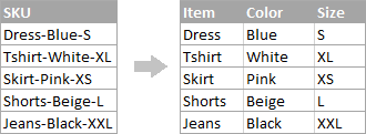
- To extract the item name (all characters before the 1st hyphen), insert the following formula in B2, and then copy it down the column:
In this formula, SEARCH determines the position of the 1st hyphen («-«) in the string, and the LEFT function extracts all the characters left to it (you subtract 1 from the hyphen’s position because you don’t want to extract the hyphen itself). 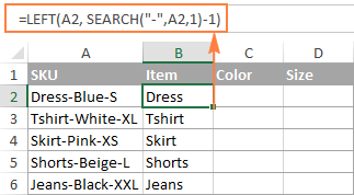
To extract the color (all characters between the 1st and 2nd hyphens), enter the following formula in C2, and then copy it down to other cells:
=MID(A2, SEARCH(«-«,A2) + 1, SEARCH(«-«,A2,SEARCH(«-«,A2)+1) — SEARCH(«-«,A2) — 1) 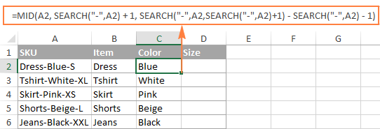
In this formula, we are using the Excel MID function to extract text from A2.
The starting position and the number of characters to be extracted are calculated with the help of 4 different SEARCH functions:
- Start number is the position of the first hyphen +1:
SEARCH(«-«,A2) + 1
Number of characters to extract: the difference between the position of the 2 nd hyphen and the 1 st hyphen, minus 1:
SEARCH(«-«, A2, SEARCH(«-«,A2)+1) — SEARCH(«-«,A2) -1
To extract the size (all characters after the 3rd hyphen), enter the following formula in D2:
=RIGHT(A2,LEN(A2) — SEARCH(«-«, A2, SEARCH(«-«, A2) + 1))
In this formula, the LEN function returns the total length of the string, from which you subtract the position of the 2 nd hyphen. The difference is the number of characters after the 2 nd hyphen, and the RIGHT function extracts them. 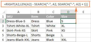
In a similar fashion, you can split column by any other character. All you have to do is to replace «-» with the required delimiter, for example space (» «), comma («,»), slash («/»), colon («;»), semicolon («;»), and so on.
Tip. In the above formulas, +1 and -1 correspond to the number of characters in the delimiter. In this example, it’s a hyphen (1 character). If your delimiter consists of 2 characters, e.g. a comma and a space, then supply only the comma («,») to the SEARCH function, and use +2 and -2 instead of +1 and -1.
How to split string by line break in Excel
To split text by space, use formulas similar to the ones demonstrated in the previous example. The only difference is that you will need the CHAR function to supply the line break character since you cannot type it directly in the formula.
Supposing, the cells you want to split look similar to this: 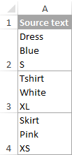
Take the formulas from the previous example and replace a hyphen («-«) with CHAR(10) where 10 is the ASCII code for Line feed.
- To extract the item name:
=LEFT(A2, SEARCH(CHAR(10),A2,1)-1)
To extract the color:
=MID(A2, SEARCH(CHAR(10),A2) + 1, SEARCH(CHAR(10),A2,SEARCH(CHAR(10),A2)+1) — SEARCH(CHAR(10),A2) — 1)
To extract the size:
=RIGHT(A2,LEN(A2) — SEARCH(CHAR(10), A2, SEARCH(CHAR(10), A2) + 1))
And this is how the result looks like: 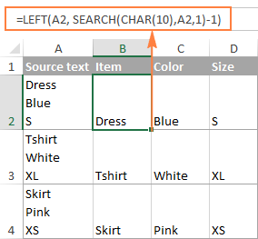
How to split text and numbers in Excel
To begin with, there is no universal solution that would work for all alphanumeric strings. Which formula to use depends on the particular string pattern. Below you will find the formulas for the two common scenarios.
Split string of ‘text + number’ pattern
Supposing, you have a column of strings with text and numbers combined, where a number always follows text. You want to break the original strings so that the text and numbers appear in separate cells, like this: 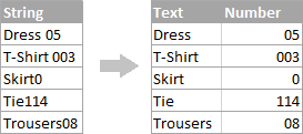
The result may be achieved in two different ways.
Method 1: Count digits and extract that many chars
The easiest way to split text string where number comes after text is this:
To extract numbers, you search the string for every possible number from 0 to 9, get the numbers total, and return that many characters from the end of the string.
With the original string in A2, the formula goes as follows:
To extract text, you calculate how many text characters the string contains by subtracting the number of extracted digits (C2) from the total length of the original string in A2. After that, you use the LEFT function to return that many characters from the beginning of the string.
Where A2 is the original string, and C2 is the extracted number, as shown in the screenshot: 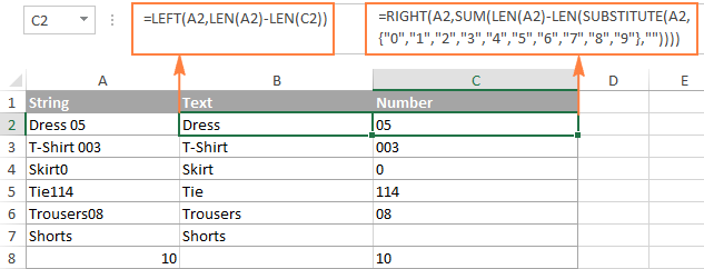
Method 2: Find out the position of the 1 st digit in a string
An alternative solution would be using the following formula to determine the position of the first digit in the string:
Once the position of the first digit is found, you can split text and numbers by using very simple LEFT and RIGHT formulas.
To extract text:
To extract number:
Where A2 is the original string, and B2 is the position of the first number. 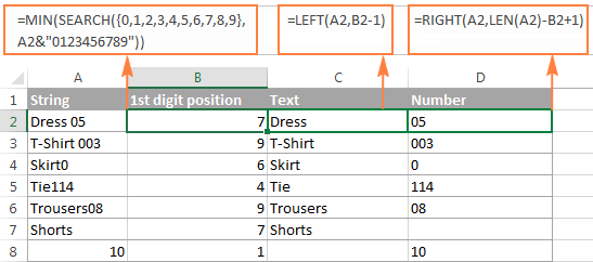
To get rid of the helper column holding the position of the first digit, you can embed the MIN formula into the LEFT and RIGHT functions:
Formula to extract text:
Formula to extract numbers:
Split string of ‘number + text’ pattern
If you are splitting cells where text appears after number, you can extract numbers with the following formula:
The formula is similar to the one discussed in the previous example, except that you use the LEFT function instead of RIGHT to get the number from the left side of the string.
Once you have the numbers, extract text by subtracting the number of digits from the total length of the original string:
Where A2 is the original string and B2 is the extracted number, as shown in the screenshot below: 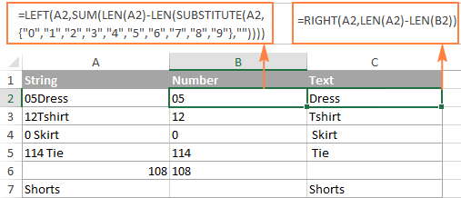
Tip. To get number from any position in a text string, use either this formula or the Extract tool. Or you can create a custom function to split numbers and text into separate columns.
This is how you can split strings in Excel using different combinations of different functions. As you see, the formulas are far from obvious, so you may want to download the sample Excel Split Cells workbook to examine them closer.
If figuring out the arcane twists of Excel formulas is not your favorite occupation, you may like the visual method to split cells in Excel, which is demonstrated in the next part of this tutorial.
How to split cells in Excel with Split Text tool
An alternative way to split a column in Excel is using the Split Text feature included with our Ultimate Suite for Excel, which provides the following options:
To make things clearer, let’s have a closer look at each option, one at a time.
Split cells by character
Choose this option whenever you want to split the cell contents at each occurrence of the specified character.
For this example, let’s the take the strings of the Item-Color-Size pattern that we used in the first part of this tutorial. As you may remember, we separated them into 3 different columns using 3 different formulas. And here’s how you can achieve the same result in 2 quick steps:
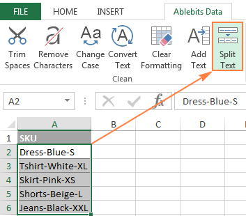
- Assuming you have Ultimate Suite installed, select the cells to split, and click the Split Text icon on the Ablebits Data tab.

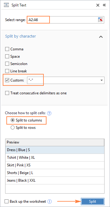
- The Split Text pane will open on the right side of your Excel window, and you do the following:
- Expand the Split by character group, and select one of the predefined delimiters or type any other character in the Custom box.
- Choose whether to split cells to columns or rows.
- Review the result under the Preview section, and click the Split button.
Tip. If there might be several successive delimiters in a cell (for example, more than one space character), select the Treat consecutive delimiters as one box.
Done! The task that required 3 formulas and 5 different functions now only takes a couple of seconds and a button click. 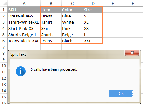
Split cells by string
This option lets you split strings using any combination of characters as a delimiter. Technically, you split a string into parts by using one or several different substrings as the boundaries of each part.
For example, to split a sentence by the conjunctions «and» and «or«, expand the Split by strings group, and enter the delimiter strings, one per line: 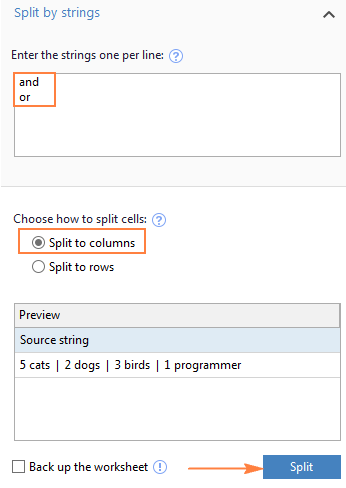
As the result, the source phrase is separated at each occurrence of each delimiter: 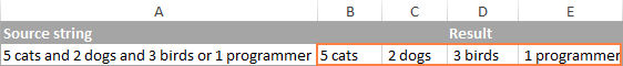
Tip. The characters «or» as well as «and» can often be part of words like «orange» or «Andalusia», so be sure to type a space before and after and and or to prevent splitting words.
And here another, real-life example. Supposing you’ve imported a column of dates from an external source, which look as follows:
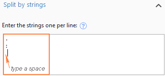
This format is not conventional for Excel, and therefore none of the Date functions would recognize any of the date or time elements. To split day, month, year, hours and minutes into separate cells, enter the following characters in the Split by strings box:
- Dot (.) to separate day, month, and year
- Colon (:) to separate hours and minutes
- Space to separate date and time
Hit the Split button, and you will immediately get the result: 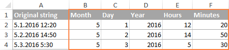
Split cells by mask (pattern)
Separating a cell by mask means splitting a string based on a pattern.
This option comes in very handy when you need to split a list of homogeneous strings into some elements, or substrings. The complication is that the source text cannot be split at each occurrence of a given delimiter, only at some specific occurrence(s). The following example will make things easier to understand.
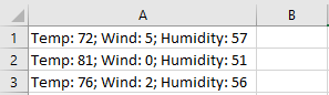
Supposing you have a list of strings extracted from some log file: 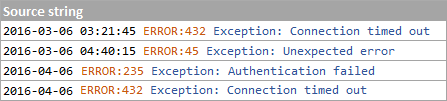
What you want is to have date and time, if any, error code and exception details in 3 separate columns. You cannot utilize a space as the delimiter because there are spaces between date and time, which should appear in one column, and there are spaces within the exception text, which should also appear in one column.
The solution is splitting a string by the following mask: *ERROR:*Exception:*
Where the asterisk (*) represents any number of characters.
The colons (:) are included in the delimiters because we don’t want them to appear in the resulting cells.
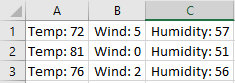
And now, expand the Split by mask section on the Split Text pane, type the mask in the Enter delimiters box, and click Split: 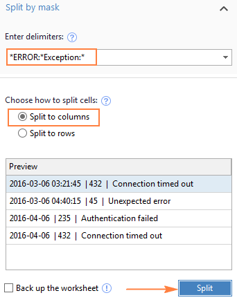
The result will look similar to this: 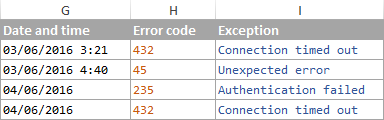
Note. Splitting string by mask is case-sensitive. So, be sure to type the characters in the mask exactly as they appear in the source strings.
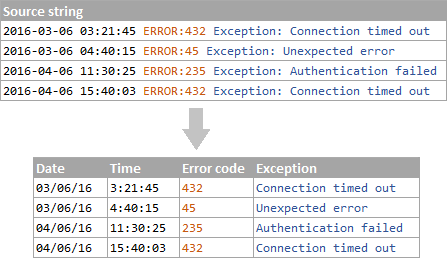
A big advantage of this method is flexibility. For example, if all of the original strings have date and time values, and you want them to appear in different columns, use this mask:
Translated into plain English, the mask instructs the add-in to divide the original strings into 4 parts:
- All characters before the 1st space found within the string (date)
- Characters between the 1 st space and the word ERROR: (time)
- Text between ERROR: and Exception: (error code)
- Everything that comes after Exception: (exception text)
I hope you liked this quick and straightforward way to split strings in Excel. If you are curious to give it a try, an evaluation version is available for download below. I thank you for reading and hope to see you on our blog next week!
Источник
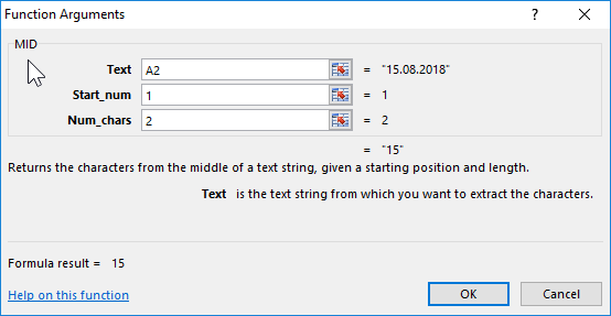
MID function in Excel is intended to select a substring from a string of text passed as the first argument, and returns the required number of characters starting from the specified position.
Examples of using the MID function in Excel
One character in single-byte-encoded languages corresponds to 1 byte. When working with such languages, the results of the functions MID and MIDB (returns a substring from a string based on the number of specified bytes) do not differ. If a two-byte language is used on the computer, each character will be counted as two characters when using MIDB. The two-byte languages are Korean, Japanese, and Chinese.
How to divide the text into several cells in columns in Excel?
Example 1. The table column contains dates recorded as text strings. Record separately in adjacent columns the number of the day, month and year, isolated from the presented dates.
View source data table:
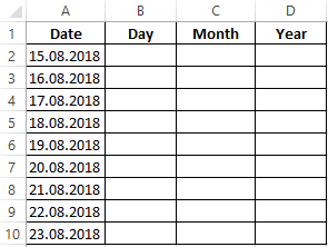
To fill in the day number, use the following formula:
Argument Description:
- A2:A10 — a range of cells with a textual representation of the dates from which the numbers of the days will be highlighted;
- 1 — the number of the initial position of the character of the extracted substring (the first character in the original string);
- 2 — the number of the last position of the character of the extracted substring.
In a similar way, we select the month numbers and years to fill in the corresponding columns, taking into account that the month number starts with the 4th character in each row and the year from the 7th. We use the following formulas:
=MID(A2:A10,4,2)
=MID(A2:A10,7,4)
View of the completed data table:
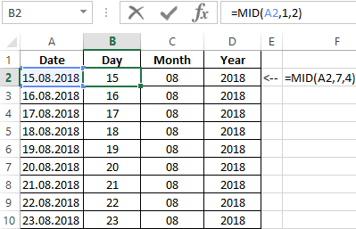
Thus, we were able to cut the text into cells of column A. It was possible to divide each date separately into several cells by columns: day, month, and year.
How to cut part of cell text in Excel?
Example 2. A text column with the name and brand of goods is stored in a table column. Split the existing lines into substrings with the name and brand, respectively, and write the values in the corresponding columns of the table.
View of data table:
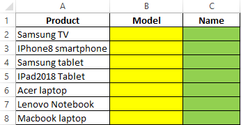
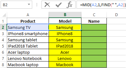
To fill the column «Name» we use the following formula:
=MID(A2,1,FIND(«»,A2))
FIND function returns the position number of the space character «» in the line being scanned, which is taken as an argument to the number_ characters of the MID function. As a result of the calculations we get:
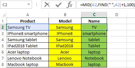
To fill the “Mark” column, use the following array formula:
=MID(A2:A8,FIND(«»,A2:A8)+1,100)
FIND function returns the position of the space character. A unit is added to the received number to find the position of the first character of the brand name of the product. The final value is used as an argument to the Start_num of the MID function. For simplicity, instead of searching for the last position number (for example, using the LEN function), the number 100 is indicated, which in this example is guaranteed to exceed the number of characters in the original line.
As a result of the calculations we get:
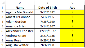
How to calculate age by date of birth in Excel?
Example 3. The table contains information about employees in the columns name and date of birth. Create a column in which the surname of the employee and his age in the format “Jon — 27” will be displayed.
View source table:
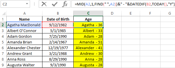
To return a string with the last name and current age, use the following formula:
MID function returns part of a string to a space character, whose position is determined by the FIND function. To find the age of the employee, use the DATEDIF function, the resulting value of which is truncated to the nearest smaller integer to get the number of full years. The TEXT function converts the resulting value to a text string.
For connection (concatenation) of the obtained strings the symbols “&” are used. As a result of the calculations we get:
Features of using the MID function in Excel
The function has the following syntax entry:
=MID(Text,Start_num,Num_chars)
Argument Description:
- Text – a required argument that accepts a cell reference with a text or a text string enclosed in quotes from which a substring of a certain length will be extracted starting from the specified position of the first character;
- Start_num – is a required argument that accepts integers from the range from 1 to N, where N is the length of the string from which you want to extract a substring of a given size. The initial position of the character in the string corresponds to the number 1. If this argument takes a fractional number from the range of valid values, the fractional part will be truncated;
- Num_chars – is a required argument that takes a value from a range of non-negative numbers, which characterizes the length in characters of the returned substring. If the argument is the number 0 (zero), the MID function returns an empty string. If the argument is a number greater than the number of characters in the string, the entire part of the string starting with the specified second position argument will be returned. In fractional numbers used as the argument, the fractional part is truncated.
MIDB function has a similar syntax:
=MIDB(Text,Start_num,Num_bytes)
It has a single argument:
- Num_bytes is a required argument that accepts integers from the range from 1 to N, where N is the bytes in the source string, characterizing the number of bytes in the returned substring.
Download examples MID function for splitting text in Excel
Notes:
- MID function will return an empty string if, as an argument, the Start_num was passed value exceeding the number of characters in the source string.
- If the value 1 was passed as an argument for Start_num, and Num_chars argument is determined by a number that is equal to or greater than the total number of characters in the source line, the MID function returns the entire line.
- If the argument Start_num was specified by a number from the range of negative numbers or 0 (by zero), the MID function will return the error code #VALUE!.
- If the Num_chars argument is a negative number, the result of the MID function is the error code #VALUE!.