Divide by one cell in excel

Excel for Microsoft 365 Excel 2021 Excel 2019 Excel 2016 Excel 2013 More…Less

You might want to split a cell into two smaller cells within a single column. Unfortunately, you can’t do this in Excel. Instead, create a new column next to the column that has the cell you want to split and then split the cell. You can also split the contents of a cell into multiple adjacent cells.

See the following screenshots for an example:

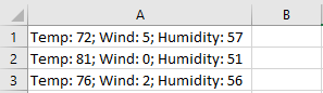
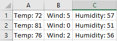
Split the content from one cell into two or more cells

Select the cell or cells whose contents you want to split.

Important: When you split the contents, they will overwrite the contents in the next cell to the right, so make sure to have empty space there.
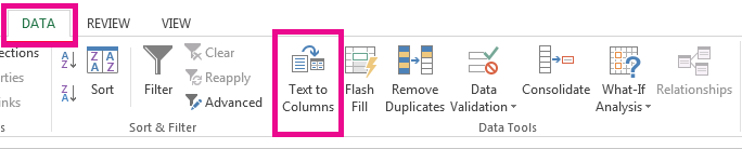
On the Data tab, in the Data Tools group, click Text to Columns. The Convert Text to Columns Wizard opens.
Choose Delimited if it is not already selected, and then click Next.
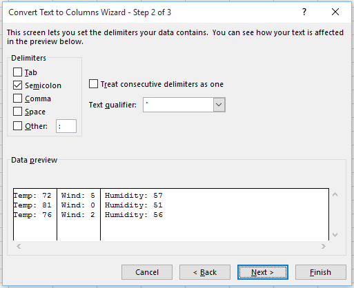
Select the delimiter or delimiters to define the places where you want to split the cell content. The Data preview section shows you what your content would look like. Click Next.
In the Column data format area, select the data format for the new columns. By default, the columns have the same data format as the original cell. Click Finish.

How do I multiply one cell by another in Excel?

How to multiply two numbers in Excel

In a cell, type “=”
Click in the cell that contains the first number you want to multiply.
Type “*”.
Click the second cell you want to multiply.
Press Enter.

What is the formula of division?

A divisor is represented in a division equation as: Dividend ÷ Divisor = Quotient. Similarly, if we divide 20 by 5, we get 4.

Why can’t I divide in Excel?

There’s no DIVIDE function in Excel. Simply use the forward slash (/) to divide numbers in Excel. 1. The formula below divides numbers in a cell.

How do you insert division in Excel?

You can insert a division symbol by shortcut key in Excel. Select a cell you will insert division symbol, hold the Alt key, type 0247 and then release the Alt key. Then you can see the ÷ symbol is showing in the selected cell. Note: The number 0247 you typed must in the numeric keypad.

What is multiply in Excel?

To multiply numbers in Excel, use the asterisk symbol (*) or the PRODUCT function.Simply use the asterisk symbol (*) as the multiplication operator. Don’t forget, always start a formula with an equal sign (=). 2. The formula below multiplies the values in cells A1, A2 and A3.

5 valid?

The formula = ((A2+B5)*5% is a proper formula.You want to paste a formula result — but not the actual underlying formula — to another cell. You would copy the cell with the formula, then place the insertion point in the cell you want to copy to.

What’s another symbol for divide?

Other symbols for division include the slash or solidus /, the colon :, and the fraction bar (the horizontal bar in a vertical fraction).

What is E $1 Excel?

In this case, the reference =E$1 in cell A1, uses relative referencing for the column and absolute referencing for the row. As shown in the results spreadsheet, the relative column reference adjusts as it is copied to other columns, but the absolute row reference remains constant.

How do you show 0 instead of DIV 0?

IFERROR is the simplest solution. For example if your formula was =A1/A2 you would enter =IFERROR(A1/A2,“”) to return a blank or =IFERROR(A1/A2,0) to return a zero in place of the error. If you prefer, use an IF statement such as =IF(A2=0,0,A1/A2). This will return a zero if A2 contains a zero or is empty.

What is divide symbol on Excel?

slash symbol
To divide in Excel you’ll need to write your formula with the arithmetic operator for division, the slash symbol (/). You can do this three ways: with the values themselves, with the cell references, or using the QUOTIENT function.

How do you divide examples?

Division is the opposite of multiplying. When we know a multiplication fact we can find a division fact: Example: 3 × 5 = 15, so 15 / 5 = 3. Also 15 / 3 = 5.

How do you divide polynomials?

Dividing Polynomials Using Long Division

Divide the first term of the dividend (4x²) by the first term of the divisor (x), and put that as the first term in the quotient (4x).
Multiply the divisor by that answer, place the product (4x² – 12x) below the dividend.
Subtract to create a new polynomial (7x – 21).

How do you add and subtract to one cell in Excel?

Subtract numbers using cell references

Type a number in cells C1 and D1. For example, a 5 and a 3.
In cell E1, type an equal sign (=) to start the formula.
After the equal sign, type C1-D1.
Press RETURN . If you used the example numbers, the result is 2. Notes:

How do you add subtract and divide in Excel?

For simple formulas, simply type the equal sign followed by the numeric values that you want to calculate and the math operators that you want to use — the plus sign (+) to add, the minus sign (-) to subtract, the asterisk (*) to multiply, and the forward slash (/) to divide.

How do you multiply in Excel without formulas?

Select the cell A1.
Copy the cell by pressing the key Ctrl+C on your keyboard.
Select the cell B1, right click with the mouse.
From the shortcut menu, select the Paste Special option.
The Paste Special dialog box will appear.
Click on Multiply in the Operation section.
Click on OK.

Источник

Excel Divide Cell (Table of Contents)

Introduction to Divide Cell in Excel
Examples of Divide Cell in Excel

Introduction to Divide Cell in Excel

When we work with the text files in excel, it has all the data in the single row itself instead of having it in different columns. The data, most of the times, is aligned in a single row with some delimiter or separator in it (such as comma, space, etc.). If you open such files in Excel, you’ll not get the data populated across columns for different attributes, which is a problem in its own ways. It makes dividing the cells into different columns extremely important, and that is exactly what we will walk you through in this article.

Data Structure in a Text File:

The data is comma-separated if you see the below screenshot and has the first row as column headers. Below that, there is one blank row and then the data values that are comma-separated as well. This type of data is called as delimited data or data with delimiters (in this case, comma as a delimiter).

Let us see the other data set which we are going to use.

This data set simply consists of EmpID and EmpName, as it seems, and there is no special delimiter in this data as well. For both of these types of data, we need to divide the cells into different columns.

Excel has a Text to Column tool, which helps us divide the cells into different columns.

Examples of Divide Cell in Excel

We will see how it works with two examples in this article.

Example #1 – Divide cells with Delimiter in Excel

See the data below. The same text file is opened with Excel, which we have seen through the above screenshots and has comma-separated values in it within a single row of the sheet.

To divide it into different columns per field value, we need to use the Text to Column utility in Excel.

Step 1: Select all the cells from column A (spread across the cells A1 to A12) containing data which is comma-separated.

Step 2: Navigate to the Data tab under the Excel ribbon, which is placed at the uppermost corner of the worksheet and click on it.

Step 3: As soon as you click on the Data tab, you’ll see different options associated with the data using which we can manipulate the data in Excel. However, you need to navigate to the Data Tools group, under which you’ll see Text to Column as an option.

As soon as you click on the Text to Column option, you’ll see Convert Text to Column Wizard popping up on your excel screen, as shown below:

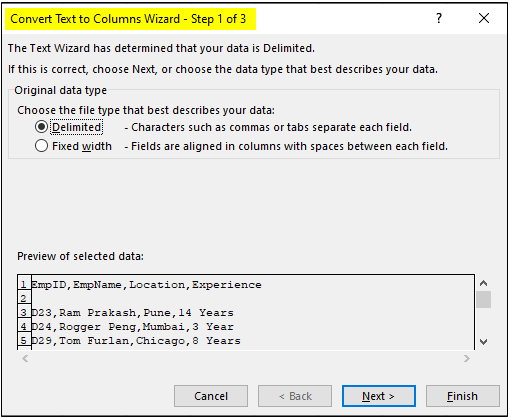
By default, the Delimited option is checked for you. Since our data has a delimiter (comma), we will go with the same selection. Click on the Next > button.

Step 4: Under the Delimiters section, tick the select Comma option (since we have comma-separated data with us). You have different delimiter options such as Tab, Semicolon, Space, etc.; if your data has any delimiter apart from these standard ones, you can use other options to add it as a delimiter for the data to be divided. Since we have a comma with us, we will use the comma as a delimiter. Once you click on the comma, you can see the cell values are divided into separate columns after each comma under the Data preview section. Click on the Next button after done.

Once you click on the next option, you’ve several options that will allow you to either change the column data type for various columns the data gets split in. Ex. Whether you wanted to store any specific column as a Text or Date format or choose not to import that column with the option, do not import the column (skip) option. Well, these are the options; right now, we are not going to use to and just will use the standard Text to Column settings, in which the Column Data Format is set as General.

Step 5: Set the Column data format as General by clicking the General radio button. Under the Destination: section set the destination as cell A1 and click on the Finish option to complete the dividing data into cells procedure.

Once you click on the Finish option, you can see data divided across different columns, as shown in the screenshot below:

You can see the data which was in a single cell with a comma as a separator or delimiter is now populated across the different columns such as EmpID (column A), EmpName (column B), Location (column C) and Experience (column D).

This is one way to divide cells in Excel when you have delimited data.

Example #2 – Divide cells with Fixed Width in Excel

The Other example is something where you don’t have any delimiter but a data with fixed with and you need to divide the cells containing that data into different columns.

See the data below:

Step 1: Follow the first three steps from the previous example (Example 1) as it is to be able to open the Text to Column Wizard in Excel, which helps in dividing the cells.

Step 2: Now, as soon as the Convert Text to Columns Wizard gets opened, you need to click the Fixed Width radio button instead of the Delimited (which is set by default). Click on the Next button.

Step 3: After you click on the Next button, you can make the split after a specific length. For Example, we can make a split after the first three characters, which are part of EmpID. See the screenshot below. After you are happy with the split made, click on the Next button.

Step 4: On the next screen, you can set the data type as General, Date, etc. And set the Destination Range as well. Once done, you can click on the Finish button. See the screenshot below:

Once you click on the Finish button, you can see the data divided into two different columns, as shown below:

This is how we can divide cells in Excel into different columns using Text to Column wizard.

Things to Remember

For dividing the cells, your data should have a common delimiter for all the fields. Otherwise, it is not possible to divide the data into different columns.
If the data doesn’t have a delimiter, you can use the Fixed Width option as well. However, your data should have a fixed number of characters where a split can happen for that to happen. For Ex. after every third character, you may create a split (as shown in Example 2.)

Method 1: splitting cells using the Delimiter with Text to Column feature

1. In an open Excel workbook, click and select all the cells you want to split.

2. from the main menu ribbon, click on the Data tab.

3. Under the Data Tools tab, select the ‘Text to Columns’ option to display the ‘Convert Text to Columns Wizard – Step 1 to 3’ dialog box.

4. In the dialog box, for step 1, check on the ‘Delimited’ option checkbox. Click Next to proceed.

5. Under the’ Delimiters’ section, step 2 of the wizard dialog box, specify the delimiter you want to split. You will be able to see a preview of any applied delimiters you select in the ‘Data preview’ field. Click Next to proceed.

6. In the 3^rd step, select a Destination for your selected cells data.

7. Click Finish. Every text or value string in that cell will split into different cells.

Method 2: splitting cells using VBA macro

1. In this example, I will split the cells with the following sentences using VBA macro

1. Go to the Developers tab and click on the ‘Visual Basic’ option or (Press Alt+F11 to access the visual basic editor)

2. The ‘Visual Basic Editor’ window will be displayed.

3. Click on the Insert tab. From the given options, select Module to create a new module

4. Type in VBA code into the ‘Code Window.’

Public Sub SplitName()

X = Cells(Rows.Count, 1).End(xlUp).Row

For A = 1 To X

B = InStr(Cells(A, 1), » «)

C = InStrRev(Cells(A, 1), » «)

Cells(A, 2) = Left(Cells(A, 1), B)

Cells(A, 3) = Mid(Cells(A, 1), B, C – B)

Cells(A, 4) = Right(Cells(A, 1), Len(Cells(A, 1)) – C)

Next A

End Sub

5. Click the Run tab and select Run Macro to display a dialog box. (Or simply press F5 to run the code)

6. In the ‘Macro’ dialog box, click the Run button.

Method 3: using the flash fill feature

1. In your open workbook, select empty cell columns right beside the main column you want to split.

2. In the first cell of the first column, type in the first value or text you want to split and press Enter.

3. Type the second name in the second cell. Flash fill feature will appear. If not Go to the Data tab on the main ribbon, click on the Flash Fill option indicating the cell you had typed in. you will see that the first part (all values or texts) in the main column has been split automatically in the adjacent column.

4. Carry on the process for the other columns to separate all text or value strings.

Method 4: splitting cells by using the unmerge cells option in Excel.

While working on imported Excel files, you may find the data merged, or some cells are combined. An easy way to split these cells is by clicking on the Unmerge Cells options. To do this;

1. In your open workbook, select all the cells you need to split.

2. In the Home tab, under the Alignment group, click on the Merge & Centre drop-down arrow.

3. Select Unmerge Cells, and this will divide your merged cells.

Conclusion

The article below gives you different methods on how to split or divide cells. As a constant Excel user who comes across cells you need to separate, you can select either of the methods above to achieve this.

Источник

Unlike the SUM function that can automatically add cells’ values in Excel, there is no predefined division function in Excel. However, there are also several ways to do this math operation in this program. To read more about how to divide in Excel, follow this post to learn basic to advanced division methods in Excel.

How to divide in Excel

Divide in Excel by using the divide symbol

The simplest way to divide in Excel is by using the divide symbol (/). You can divide numbers into one cell or divide the amounts of multiple cells. We are going to explain each of them as follow:

First, to divide two amounts in one cell:

Select the cell that you want to apply the divide operation to.
Every formula in Excel should start with “=” so, write this symbol first.
Write the first number, and without any space, write / and then the second number.
Press Enter to see the result.

Figure 1- Dividing two numbers in one cell in Excel

Remember, writing formulas with this method is not always useful. It is more practical to divide the amounts of two different cells. Consequently, if you change the value of each cell, the result will change.

First, write the number in different cells.

Figure 2- Dividing values of two cells in Excel

Select the third cell where you want to display the result. It can be any cell on the sheet. (in our example we chose B5)
Start the formula by writing an equal sign “=”.
Select the first cell by clicking on it. (in our example it is B3)
Write “/” and select the second cell. (in our example is B4)

Figure 3- Write the division formula in the third cell where you want to see the result

Press Enter to see the result.

Figure 4- You can see the result of the division in the cell where you have written the formula

Whenever you modify the value of the cells (in our example B3 and B4), the number in the third cell (here B5) will change. But you can’t write anything in the cells that have formulas. If you double-click on it, you can only see the formula.

Divide from one cell

Sometimes you may need to divide the value of different cells from the same number. For example, all the cells of one column should be divided into 3.

Select the cell where you want to see the result. Write an equal symbol “=” and select the first cell.
Add “/” to the formula and then select the cell that you have written the number. Then press Enter.

Figure 5- Dividing the values of a column from one cell

Although it’s possible to write the formula for each cell one by one, it’s easier to fix the cell where you input the number (in this example, D3). So, you can copy the formula for other cells.

Go to the formula and put the cursor behind the cell name (D3) and press F4. You can see that two dollar signs appear, one before the cell name and the other after that. It shows that this cell (D3) is locked and won’t change by copying.

Figure 6- The dollar signs indicate that the cell is locked

You can either double-click on the right corner of the cell to copy it to all the other cells which have values or simply drag it down.

Figure 7- Even after copying the cells, the D3 value remained the same

What happens if you don’t lock the cell in this formula?

Figure 8-DIV/O! Error in Excel!

If you don’t lock the cell you want to remain the same for all the formulas, you will face the DIV/O! Error, which displays when the value of the cell you want to divide from equals zero or is not a number at all. Read more on Excel Formula Errors and why they occur.

How to Solve #DIV/0!

Since dividing a number by zero is not defined, Excel shows the #DIV/0! Error. A textual or an empty cell will be given a zero value in mathematical calculations in Excel. So, we prefer excel shows the open cell instead of a cell that contains an error.

IFERROR Function

By using the IFERROR function, you can solve the #DIV/0! Error. When you write the formula, you can add this function and define a second parameter to represent it instead of the error. Here are the steps to use this function:

Select a cell or column (based on the numbers of your dataset.)
Write the equal sign.
Write IFERROR()
As the first argument, write the divide formula (as we mentioned before.)
As the second argument, write the parameter between “”

For instance, don’t write anything if you want excel to show an empty cell.

=IFERROR(the divide formula, “”)

Figure 9- IFERROR Function

Divide with Paste Special option

As mentioned earlier, if you write a formula in a cell, you’ll see the formula by clicking on it. But, it is also possible to see the value, not the formula. In this case, you should use the Paste Special option. Follow the instruction below:

Figure 12- The result of division in Excel using the Paste Special option.

There is one problem with this method of division in Excel. Since you don’t have any formula, if you change the value of the first cells, the result will not change. That makes it a first-time division method, and it’s not dynamic like the division formula in Excel.

Bottom Line

The division is one of the main mathematical operations that are very useful in accounting functions or making different dynamic reports. We explained how to divide in Excel step by step. So, with a little creativity, you can easily use this operation in Excel.

Check out our other blogs, explaining the other three basic arithmetic operations in Excel:

How to Add Numbers, Cells, and Columns in Excel
How to Sum in Excel
How to Subtract in Excel
How to Multiply in Excel

Источник

Split the content from one cell into two or more cells

See Also

Need more help?

How do I multiply one cell by another in Excel?

What is the formula of division?

Why can’t I divide in Excel?

How do you insert division in Excel?

What is multiply in Excel?

5 valid?

What’s another symbol for divide?

What is E $1 Excel?

How do you show 0 instead of DIV 0?

What is divide symbol on Excel?

How do you divide examples?

How do you divide polynomials?

How do you add and subtract to one cell in Excel?

How do you add subtract and divide in Excel?

How do you multiply in Excel without formulas?

Introduction to Divide Cell in Excel

Examples of Divide Cell in Excel

Example #1 – Divide cells with Delimiter in Excel

Example #2 – Divide cells with Fixed Width in Excel

Things to Remember

Recommended Articles

Method 1: splitting cells using the Delimiter with Text to Column feature

Method 2: splitting cells using VBA macro

Method 3: using the flash fill feature

Method 4: splitting cells by using the unmerge cells option in Excel.

Conclusion

How to divide in Excel

Divide in Excel by using the divide symbol

Divide from one cell

How to Solve #DIV/0!

IFERROR Function

Divide with Paste Special option

Bottom Line