Divide all columns excel

To divide columns in Excel, just do the following:

1. Divide two cells in the topmost row, for example: =A2/B2.
2. Insert the formula in the first cell (say C2) and double-click the small green square in the lower-right corner of the cell to copy the formula down the column. Done!

How do I divide a column by 10 in Excel?

Enter the certain number in a blank cell (for example, you need to multiply or divide all values by number 10, then enter number 10 into the blank cell). Copy this cell with pressing the Ctrl + C keys simultaneously. 2. Select the number list you need to batch multiply, then click Home > Paste > Paste Special.

What is the formula for an entire column in Excel?

To add up an entire column, enter the Sum Function: =sum( and then select the desired column either by clicking the column letter at the top of the screen or by using the arrow keys to navigate to the column and using the CTRL + SPACE shortcut to select the entire column. The formula will be in the form of =sum(A:A).

How do I split a whole column in sheets?

Using the DIVIDE Formula
Click on an empty cell and type =DIVIDE(,) into the cell or the formula entry field, replacing and with the two numbers you want to divide. Note: The dividend is the number to be divided, and the divisor is the number to divide by.

How do you auto multiply in Excel?

How to multiply two numbers in Excel

1. In a cell, type “=”
2. Click in the cell that contains the first number you want to multiply.
3. Type “*”.
4. Click the second cell you want to multiply.
5. Press Enter.
6. Set up a column of numbers you want to multiply, and then put the constant in another cell.

What is the division formula?

The division formula is used for splitting a number into equal parts. Symbols that we use to indicate division are (÷) and (/). Thus, “p divided by q” can be written as: (p÷q) or (p/q).

How do you apply formula to entire column in Excel without dragging?

7 Answers

1. First put your formula in F1.
2. Now hit ctrl+C to copy your formula.
3. Hit left, so E1 is selected.
4. Now hit Ctrl+Down.
5. Now hit right so F20000 is selected.
6. Now hit ctrl+shift+up.
7. Finally either hit ctrl+V or just hit enter to fill the cells.

How do you select an entire column?

To select an entire column, click the column letter or press Ctrl+spacebar.

What is multiply in Excel?

To multiply numbers in Excel, use the asterisk symbol (*) or the PRODUCT function.Simply use the asterisk symbol (*) as the multiplication operator. Don’t forget, always start a formula with an equal sign (=). 2. The formula below multiplies the values in cells A1, A2 and A3.

How do you divide columns in numbers?

Divide a column of numbers by a constant number
In this example, the number you want to divide by is 3, contained in cell C2. Type =A2/$C$2 in cell B2. Be sure to include a $ symbol before C and before 2 in the formula. Drag the formula in B2 down to the other cells in column B.

How do I split a cell in sheets?

Split Cells with Menu Option

1. Select the cell you want to split, then go to the Data menu and choose the Split Text To Columns option.
2. Your data will be automatically split into columns. Note that Google Sheets will look at the data and try to determine what character to use as a separator to split the text.

What is the shortcut to divide in Excel?

You can insert a division symbol by shortcut key in Excel. Select a cell you will insert division symbol, hold the Alt key, type 0247 and then release the Alt key. Then you can see the ÷ symbol is showing in the selected cell. Note: The number 0247 you typed must in the numeric keypad.

How do you add and divide in the same cell in Excel?

To enter the formula:

1. Type an equal sign ( = ) in cell B2 to begin the formula.
2. Select cell A2 to add that cell reference to the formula after the equal sign.
3. Type the division sign ( / ) in cell B2 after the cell reference.
4. Select cell A3 to add that cell reference to the formula after the division sign.

How do I apply a formula to an entire column?

The easiest way to apply a formula to the entire column in all adjacent cells is by double-clicking the fill handle by selecting the formula cell. In this example, we need to select the cell F2 and double click on the bottom right corner. Excel applies the same formula to all the adjacent cells in the entire column F.

How do I apply a formula to an entire column except the first row?

Select the header or the first row of your list and press Shift + Ctrl + ↓(the drop down button), then the list has been selected except the first row.

How do I fill an entire column with the same value?

Place the cursor in the bottom right corner of the cell you just typed in until you see a plus sign. With the left mouse button, press and drag the Fill Handle (plus sign) to highlight all of the cells you want filled. Release the mouse button and the cells are filled with the value typed in the first cell.

What is the shortcut to select an entire column in Excel?

Ctrl+Space is the keyboard shortcut to select an entire column.

How do I select an entire column in Excel without the header?

If you want to select Entire Column except Header row and also excluding all blank cells in your worksheet, you can use a shortcut keys to achieve the result. Just select the first cell except header cell, and press Shift + Ctrl + Down keys.

See all How-To Articles

This tutorial will demonstrate how to divide cells and columns in Excel and Google Sheets.

The Divide Symbol

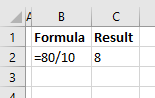
The divide symbol in Excel is the forward slash on the keyboard (/). This is the same as using the division sign (÷) in mathematics. When you divide two numbers in Excel, start with an equal sign (=), which will create a formula. Then type in the first number (the number you want to divide), followed by the forward slash, and then the number you wish to divide by.

=80/10

The result of this formula would then be 8.

Divide With a Cell Reference and a Constant

For greater flexibility in your formula, use the reference of a cell as the number to be divided and a constant as the number to divide by.

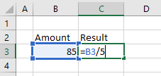
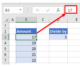
To divide B3 by 5, type the formula:

=B3/5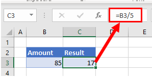

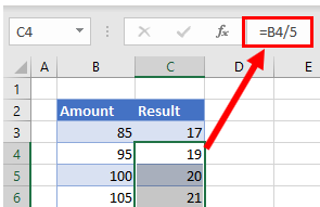
Then copy this formula down the column to the rows below. The constant number (5) will remain the same but the cell address for each row will change according to the row you are in due to Relative Cell referencing.

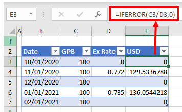
Divide a Column With Cell References

You can also use a cell reference for the number to divide by.

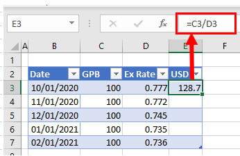
To divide cell C3 by cell D3, type the formula:

=C3/D3

Since the formula uses cell addresses, you can then copy this formula down to the rest of the rows in the table.

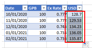
As the formula uses Relative Cell addresses, the formula will change according to the row it is copied down to.

Note: that you can also divide numbers in Excel by using the QUOTIENT Function.

Divide a Column With Paste Special

You can divide a column of numbers by a divisor, and return the result as a number within the same cell.

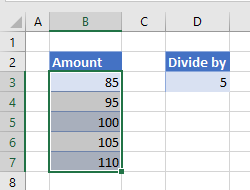
1. Select the divisor (in this case, 5) and in the Ribbon, go to Home > Copy, or press CTRL + C.

1. Highlight the cells to be divided (in this case B3:B7).

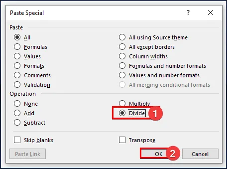
1. In the Ribbon, go to Home > Paste > Paste Special.

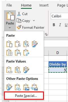
1. In the Paste Special dialog box, select Divide and then click OK.

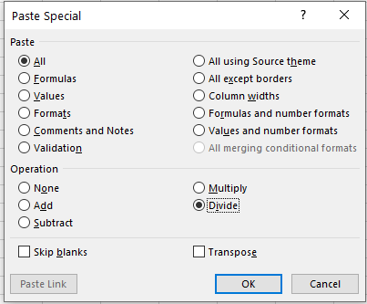
The values in the highlighted cells will be divided by the divisor that was copied and the result will be returned in the same location as the highlighted cells. In other words, you will overwrite your original values with the new divided values; cell references are not used in this this method of calculation.

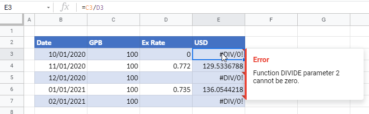
The #DIV/0! Error

If you try and divide a number by zero, you will get an error as there is no answer when a number is divided by zero.

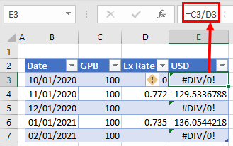
You will also get an error if you try and divide a number by a blank cell.

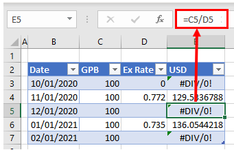
To prevent this from happening, you can use the IFERROR Function in your formula.

Using the methods above, you can also add, subtract, or multiply cells and columns in Excel.

How to Divide Cells and Columns in Google Sheets

Apart from the divide Paste Special function (which does not work in Google Sheets), all of the above examples will work in exactly the same way in Google Sheets.

You might want to split a cell into two smaller cells within a single column. Unfortunately, you can’t do this in Excel. Instead, create a new column next to the column that has the cell you want to split and then split the cell. You can also split the contents of a cell into multiple adjacent cells.

See the following screenshots for an example:

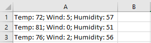
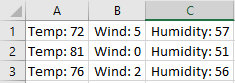
Split the content from one cell into two or more cells

1. Select the cell or cells whose contents you want to split.

   Important: When you split the contents, they will overwrite the contents in the next cell to the right, so make sure to have empty space there.

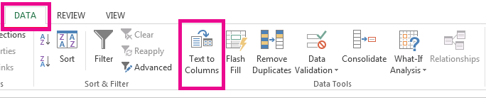
2. On the Data tab, in the Data Tools group, click Text to Columns. The Convert Text to Columns Wizard opens.

   

3. Choose Delimited if it is not already selected, and then click Next.

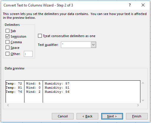
4. Select the delimiter or delimiters to define the places where you want to split the cell content. The Data preview section shows you what your content would look like. Click Next.

   

5. In the Column data format area, select the data format for the new columns. By default, the columns have the same data format as the original cell. Click Finish.

See Also

Merge and unmerge cells

Merging and splitting cells or data

Do you have any tricks on how to split columns in excel? When working with Excel, you may need to split grouped data into multiple columns. For instance, you might need to separate the first and last names into separate columns. 

With Excel’s “Text to Feature” there are two simple ways of splitting your columns. If there is an evident delimiter such as a comma, use the “Delimited” option. However, the “Fixed method is ideal for splitting the columns manually.”

To learn how to split a column in excel and make your worksheet easy-to-read, follow these simple steps. You can also check our Microsoft Office Excel Cheat Sheet here. But, first, why should you split columns in excel? 

Jump to:

• Why you need to split cells
• How do you split a column in excel?
• Method 1- Delimited Option
• Method 2- Fixed Width
• How to Split One Column into Multiple Columns in Excel
• Method 3- Split Columns by Flash Fill
• Method 4- Use LEFT, MID and RIGHT text string functions 

Why you need to split cells

If you downloaded a file that Excel can’t divide, then you need to separate your columns. You should split a column in excel if you want to divide it with a specific character. Some examples of familiar characters are commas, colons, and semicolons.

How do you split a column in excel?

Method 1- Delimited Option

This option works best if your data contains characters such as commas or tabs. Excel only splits data when it senses specific characters such as commas, tabs, or spaces. If you have a Name column, you can separate it into First and Last name columns

1. First, open the spreadsheet that you want to split a column in excel
2. Next, highlight the cells to be divided. Hold the SHIFT key and click the last cell on the range
3. Alternatively, right-click and drag your mouse to highlight the cells
4. Now, click the Data tab on your spreadsheet.
5. Navigate to and click on the “Text to Columns” From the Convert Text to Columns Wizard dialog box, select Delimited and click “Next.”
6. Choose your preferred delimiter from the options given and click “Next.”
7. Now, highlight General as your Column Data Format
8. “General” format converts all your numeric values to numbers. Date values are converted to dates, and the rest of the data is converted to text. “Text” format only converts the data into text. “Date” allows you to select your desired date format. You can skip the column by choosing “Do not import column.” 
9. Afterward, type the “Destination” field for your new column. Otherwise, Excel will replace the initial data with the divided data
10. Click “Finish” to split your cells into two separate columns.

Method 2- Fixed Width 

This option is ideal if spaces separate your column data fields. So, Excel splits your data based on the character counts, be it 5th or 10th characters.  

1. Open your spreadsheet and select the column you wish to split. Otherwise, the “Text Columns” will be inactive. 
2. Next, click Text Columns in the “Data” Tab
3. Click Fixed Width and then Next
4. Now you can adjust your column breaks in the “Data preview.” Unlike the “Delimited” option that focuses on characters, in “Fixed Width,” you select the position of splitting the text.
5. Tips: Click the preferred position to CREATE a line break. Double-Click on the line to delete it. Click and drag a column break to move it
6. Click Next if you’re satisfied with the results
7. Select your preferred Column Data Format 
8. Next, type the “Destination” field for your new column. Otherwise, Excel will replace the initial data with the divided data.
9. Finally, click Finish to confirm the changes and divide your column into two

How to Split One Column into Multiple Columns in Excel

A single column can be split into multiple columns using the same steps outlined in this guide

Tip: The number of columns depends on the number of delimiters that you select. For instance, Data will be split into three columns if it contains three commas.

Method 3- Split Columns by Flash Fill

If you are using Excel 2013 and 2016, you are in luck. These versions are integrated with a Flash fill feature that extracts data automatically once it recognizes a pattern. You can use flash fill to split the first and last name in your column. Alternatively, this feature combines separate columns into one column.

If you don’t have these professional versions, quickly upgrade your Excel version. Follow these steps to divide your columns using Flash Fill. 

• Assume your data resembles the one in the image below

• Next, in cell B2, type the First Name as below

• Navigate to the Data Tab and click Flash Fill. Alternatively, use the shortcut CTRL+E
• Selecting this option automatically separates all the First Names from the given column

Tip: Before clicking Flash Fill, ensure that cell B2 is selected. Otherwise, a warning appears that

• Flash Fill cannot recognize a pattern to extract the values. Your extracted values will look like this: 

 

• Apply the same steps for the last name as well.

 

Now, you have learned to split a column in excel into multiple cells 

Method 4- Use LEFT, MID and RIGHT text string functions 

Alternatively, use LEFT, MID, and RIGHT string functions to split your columns in Excel 2010, 2013 and 2016. 

• LEFT function: Returns the first character or characters on your left, depending on the specific number of characters you require.
• MID Function: Returns the middle number of characters from string text beginning from where you specify.
• RIGHT Function: Gives the last character or characters from your text field, depending on the specified number of characters on your right.

However, this option is not valid if your data contains a formula such as VLOOKUP. In this example, you’ll learn how to split Address, City, and zip code columns.

 

To extract the Addresses using the LEFT function:

1. First select cell B2
2. Next, apply the formula =LEFT(A2,4)

Tip: 4 represents the number of characters representing the address

    3. Click, hold and drag down the cell to copy the formula to the entire column

To extract the City data, use the MID function as follows:

• First, Select cell C2
• Now, apply the formula =MID(A2,5,2)

Tip: 5 represents the fifth character. 2 is the number of characters representing the city.

• Right-click and drag down the cell to copy the formula in the rest of the column

Finally, to extract the last characters in your data, use the Right text function as follows:

• Select Cell D2
• Next, apply the formula =RIGHT(A2,5)

Tip: 5 represents the number of characters representing the Zip Code

• Click, hold and drag down the cell to copy the formula in the entire column

Tips to remember

• The shortcut key for Flash Fill is CTRL+E
• Always try to identify a shared value in your column before splitting it
• Familiar characters when splitting columns include commas, tabs, semicolons, and spaces. 

Text Columns is the best feature to split a column in excel. It might take you several attempts to master the process. But once you get the hang of it, it will only take you a couple of seconds to split your columns. The results are professional, clean, and eye-catching columns. 

 If you’re looking for a software company you can trust for its integrity and honest business practices, look no further than SoftwareKeep. We are a Microsoft Certified Partner and a BBB Accredited Business that cares about bringing our customers a reliable, satisfying experience on the software products they need.   We will be with you before, during, and after all the sales.

How-To

In this article, I will show how to divide columns in Excel. I will show several ways. Choose one that best suits your job.So, lets start.Table of Contents hideDivision Symbol in E

Nov 16, 2022
• 8 min read

In this article, I will show how to divide columns in Excel. I will show several ways. Choose one that best suits your job.

So, lets start.

---

Table of Contents hideDivision Symbol in ExcelHow to Divide in ExcelDownload Practice Workbook8 Handy Ways to Divide Columns in Excel1. Dividing a Cell by Another Cell or Number in Excel2. Copying Formula to Divide Columns in Excel3. Applying Array formula to Divide Columns4. Using Formula to Divide Columns4.1.Using the Hard-coded Number4.2. Using Dynamic Method5. Utilizing Paste Special Feature to Divide Columns6. Inserting QUOTIENT Function to Divide Columns7. Using Percentage to Divide Columns8. Applying VBA Code to Divide ColumnsSpecial Notes to RememberConclusionRelated Articles

Division Symbol in Excel

In mathematics, to divide two numbers we use an obelus symbol (÷).

15 ÷ 5 = 3

But in Excel, we use the forward-slash (/) to divide two numbers.

15/5 = 3

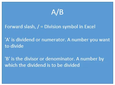
In Excel, we write a division expression like the above image, where:

• A is the dividend or numerator  a number you want to divide by another number (divisor).
• B is the divisor or denominator  a number by which you want to divide another number (dividend).

---

How to Divide in Excel

Here are some examples of division in Excel.

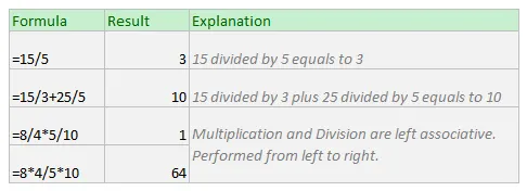
To know more about operator precedence and associativity in Excel, read this article: What is the Order & Precedence of Operations in Excel?

---

Download Practice Workbook

You may download the following Excel workbook for better understanding and practice it by yourself.Divide Columns. xlsm

---

8 Handy Ways to Divide Columns in Excel

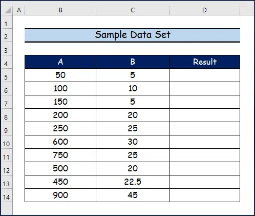
In the following methods here, we will demonstrate to you how to divide columns in Excel using 8 different ways, such as dividing a cell by another cell or number, copying the formula, applying the Array formula, using the formula, utilizing the Paste Special feature, inserting the QUOTIENT function, using percentage, and applying VBA code. Lets suppose we have a sample data set.

---

1. Dividing a Cell by Another Cell or Number in Excel

Dividing a cell by another cell or number is the same as dividing two numbers in Excel.

In the place of numbers, we just use cell references. Cell references can be relative, absolute, or mixed.

Step 1:

Here are some examples of dividing cells by another cell or number (image below).

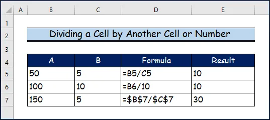
• Dividing a cell into another cell.=B5/C5
• Dividing a cell by value.=B6/5
• Dividing a cell into another cell (cell reference is absolute).= $B$7/$C$7

Read More: How to Divide Without Using a Function in Excel (with Quick Steps)

---

2. Copying Formula to Divide Columns in Excel

Step 1:

We want to divide the values of column B by the values of column C.

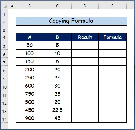
Step 2:

• Firstly select cell D5, and use this formula.=B5/C5

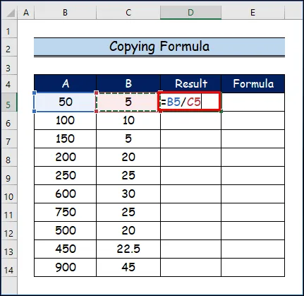
Step 3:

• Then, press Enter. The formula outputs 10 as 50 divided by 5 returns 10. Then, we select cell D5. And copy the formula in the D5 to the other cells below holding and dragging the Excels autofill handle tool. Or you can just double-click on the autofill handle tool.

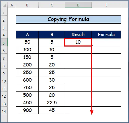
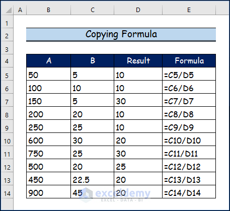
Step 4:

• And, here is the result. On the right side, the formula is shown.

---

3. Applying Array formula to Divide Columns

Lets divide a column by another one using Excels array formula. Most general Excel users fear of Excels Array Formula. If youre one of them, read this article: Excel Array Formula Basic: What is an Array in Excel?

If you want to keep safe your Excel formula from being altered or deleted by your users, you can use the array formula.

Let me show how you could perform the above calculations using an array formula.

Step 1:

• Firstly, select the cell range D5 to D14 and I type this formula.=B5:B14/C5:C14

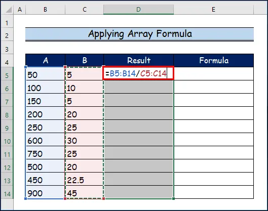
Step 2:

• Now, press CTRL + SHIFT + ENTER (I remember it with the short form CSE) simultaneously. This is the way to make an array formula in Excel. You see the results.

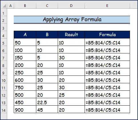
Notes

• All the cells (D5:D14) are holding the same formula. So, you cannot change the formula of a single cell. To change the formula, you have to select all the cells, and then you can edit or delete the formula. After Editing or Deleting the formula, you have to press simultaneously CTRL + SHIFT + ENTER again.

---

4. Using Formula to Divide Columns

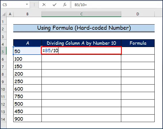
4.1.Using the Hard-coded Number

Suppose you want to divide the values of a column by a specific number 10 (it can be any).

Step 1:

• Firstly, select cell C5, and use this formula.=B5/10

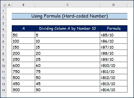
Step 2:

• So, hit Enter and then use the formula for the other cells below.
• Finally, you will see the output here.

So, the values of column B are divided by a specific number, 10.

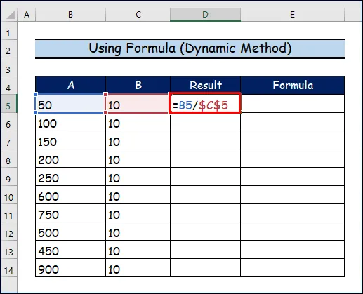
4.2. Using Dynamic Method

Maybe one day, you might want to divide those numbers by another number, say 5. It is not wise to edit the formula to get results.

We can use this method.

Step 1:

• Firstly select cell D5, and use this formula=B5/$C$5
• Therefore, from cell C5 to C14, I will place the number that will be used to divide the values of column B.
• Then, observe the formula. You see I have made the from cell C5 to C14 cell reference absolute from cell C5 to C14 as I dont want it to be changed when I use the formula for other cells in the column.

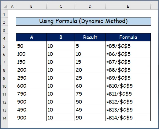
Step 2:

• Then, press Enter, and use the formula for other cells in the column.
• As a result, you will observe the results here in the below image.

---

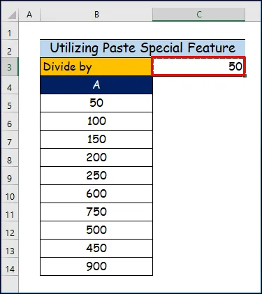
5. Utilizing Paste Special Feature to Divide Columns

In this method, you can divide a column by a specific number without using an Excel formula.

We shall use Excels Paste Special feature.

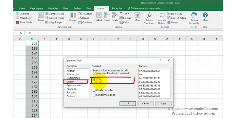
Step 1:

• Firstly, we will place the divisor in a cell. Suppose in our case, the divisor is in cell C3. Select the cell and copy the value of the cell (keyboard shortcut CTRL + C) command.

Step 2:

• Similarly, we will select the numbers under column B -> Right-click on my mouse. A menu will appear -> From the menu, click on the Paste Special.

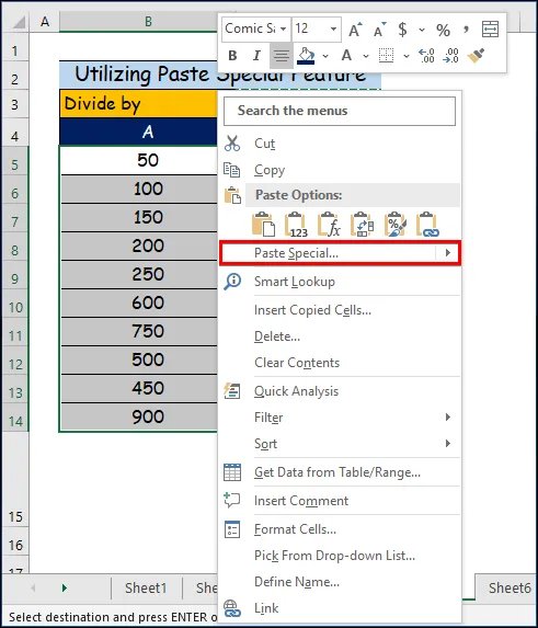
Notes

• Keyboard shortcut to open the Paste Special dialog box: CTRL + ALT + V.

Step 3:

• Then, Paste Special dialog box will appear. In this dialog box, select the Divide option (lower right corner of the dialog box). Finally, click on

Step 4:

• Therefore, here is the final result.

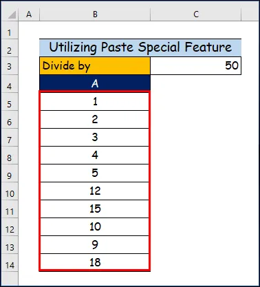
All the numbers are replaced by the new values (divided by 50). As a result, no formulas are seen in the cells.

Read More: How to Divide for Entire Row in Excel (6 Simple Methods)

---

6. Inserting QUOTIENT Function to Divide Columns

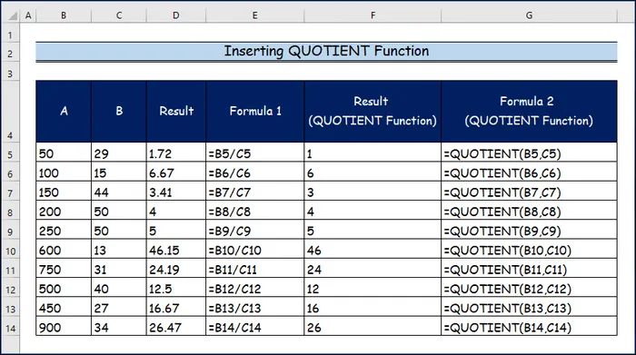
Excels QUOTIENT function returns only the integer portion of a division.

Steps:

• Here is the syntax of the QUOTIENT function.=QUOTIENT(numerator, denominator)

Check out the differences between the results done with the general Excel formula and using the QUOTIENT function.

Read More: How to Divide with Decimals in Excel (5 Suitable Examples)

7. Using Percentage to Divide Columns

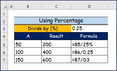
You know 25% = 25/100 = 0.25

So, dividing a column by percentage is actually the same as dividing a column by a number.

Steps:

• Here are some examples of dividing a column by percentages.=B5/25% = 200
  =B6/0.25 = 400
  =B7/D3 = 600

Read More: How to Divide a Value to Get a Percentage in Excel (5 Suitable Examples)

---

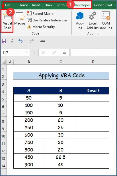
8. Applying VBA Code to Divide Columns

VBA is a programming language that may be used for a variety of tasks, and different types of users can use it for those tasks. Using the Alt + F11 keyboard shortcut, you can launch the VBA editor. In the last section, we will generate a VBA code that makes it very easy to divide columns in Excel.

Step 1:

• Firstly, we will open the Developer tab.
• Then, we will select the Visual Basic command.

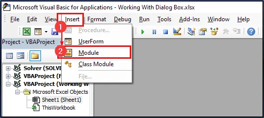
Step 2:

• Here, the Visual Basic window will open.
• After that, from the Insert option, we will choose the new Module to write a VBA code.

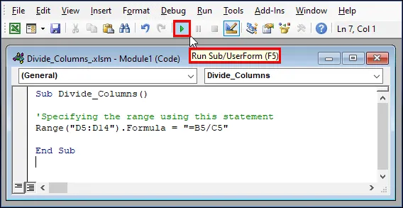
Step 3:

• Firstly, paste the following VBA code into the Module.
• Then, click the Run button or press F5 to run the program.Sub Divide_Columns() Range(«D5:D14»).Formula = «=B5/C5» End Sub

Step 4:

• Finally, as you can see, that the D column will demonstrate all the results here.

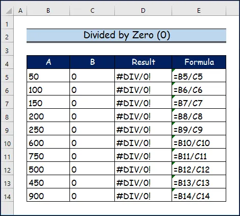
Special Notes to Remember

• You cannot divide a number by zero. This is not allowed in mathematics.
• When you try to divide a number by zero, Excel shows #DIV/0! Error.

Therefore, we can handle this error in two ways:

1. Using the IFERROR function.
2. Using the IF function.

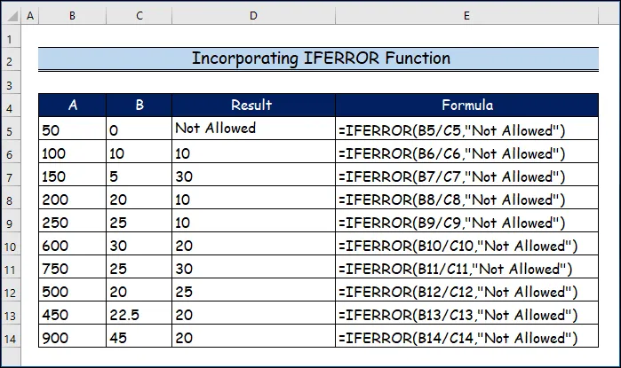
Handling #DIV/0! Error Using IFERROR function

Here is the syntax of the IFERROR function:=IFERROR (value, value_if_error)

Here, you will see how we apply the IFERROR function to handle the #DIV/0! Error in Excel.

Then, I will use this formula in cell D2.=IFERROR(B5/C5, «Not allowed»)

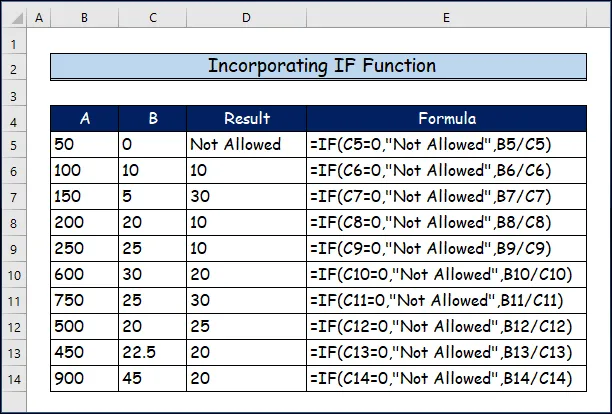
Handling #DIV/0! Error using the IF function

Here is the syntax of the IF function:

=IF(logical_test, [value_if_true], [value_if_false])

Besides, instead of using the IFERROR function, you can also use the IF function to handle the #DIV/0! Error (following image).

Then, in cell D2, I used this formula.=IF(C5=0, «Not allowed», B5/C5)

Then, I will copy-paste this formula to other cells in the column.

Read More: [Fixed] Division Formula Not Working in Excel (6 Possible Solutions)

---

Conclusion

In this article, weve covered 8 handy methods to divide columns in Excel. We sincerely hope you enjoyed and learned a lot from this article. Additionally, if you want to read more articles on Excel, you may visit our website, Exceldemy. If you have any questions, comments, or recommendations, kindly leave them in the comment section below.

---

Related Articles

• How to Add and Then Divide in Excel (5 Suitable Examples)
• Divide One Column by Another in Excel (7 Quick Ways)

Video liên quan