
Excel for Microsoft 365 Excel 2021 Excel 2019 Excel 2016 Excel 2013 More…Less
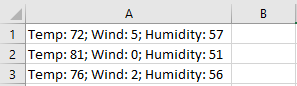
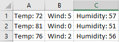
You might want to split a cell into two smaller cells within a single column. Unfortunately, you can’t do this in Excel. Instead, create a new column next to the column that has the cell you want to split and then split the cell. You can also split the contents of a cell into multiple adjacent cells.
See the following screenshots for an example:
Split the content from one cell into two or more cells
-
Select the cell or cells whose contents you want to split.
Important: When you split the contents, they will overwrite the contents in the next cell to the right, so make sure to have empty space there.
-
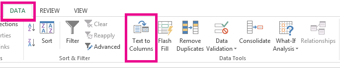
On the Data tab, in the Data Tools group, click Text to Columns. The Convert Text to Columns Wizard opens.

-
Choose Delimited if it is not already selected, and then click Next.
-
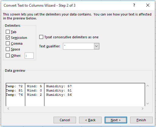
Select the delimiter or delimiters to define the places where you want to split the cell content. The Data preview section shows you what your content would look like. Click Next.
-
In the Column data format area, select the data format for the new columns. By default, the columns have the same data format as the original cell. Click Finish.
See Also
Merge and unmerge cells
Merging and splitting cells or data
Need more help?
Want more options?
Explore subscription benefits, browse training courses, learn how to secure your device, and more.
Communities help you ask and answer questions, give feedback, and hear from experts with rich knowledge.
We are used to working with whole excel cells within columns and rows. At times, you find yourself working with data imported from other sources or even working with data that is not in the format you are used to. Such data can appear in one cell alone (especially when working with texts with limited commas). Most beginners using Microsoft Excel spreadsheets may not be aware that it is possible to split a cell into two or multiple smaller ones to solve such a dilemma. Unfortunately, I do not mean to split one cell into two or numerous cells figuratively. By dividing cells in Excel, we suggest adding a new column, changing the column widths, and merging two cells into one.
Splitting excels cells helps provide better sorting and filtering features for your data. Using the Unmerge Cells, Text to Column feature, and Flash Fill features, you will be able to split Excel cells. In this article, we learn how to separate Excel cells using different methods. Let’s get started.
Method 1: splitting cells using the Delimiter with Text to Column feature
1. In an open Excel workbook, click and select all the cells you want to split.
2. from the main menu ribbon, click on the Data tab.

3. Under the Data Tools tab, select the ‘Text to Columns’ option to display the ‘Convert Text to Columns Wizard – Step 1 to 3’ dialog box.

4. In the dialog box, for step 1, check on the ‘Delimited’ option checkbox. Click Next to proceed.

5. Under the’ Delimiters’ section, step 2 of the wizard dialog box, specify the delimiter you want to split. You will be able to see a preview of any applied delimiters you select in the ‘Data preview’ field. Click Next to proceed.

6. In the 3rd step, select a Destination for your selected cells data.

7. Click Finish. Every text or value string in that cell will split into different cells.

Method 2: splitting cells using VBA macro
1. In this example, I will split the cells with the following sentences using VBA macro

1. Go to the Developers tab and click on the ‘Visual Basic’ option or (Press Alt+F11 to access the visual basic editor)

2. The ‘Visual Basic Editor’ window will be displayed.
3. Click on the Insert tab. From the given options, select Module to create a new module

4. Type in VBA code into the ‘Code Window.’
Public Sub SplitName()
X = Cells(Rows.Count, 1).End(xlUp).Row
For A = 1 To X
B = InStr(Cells(A, 1), » «)
C = InStrRev(Cells(A, 1), » «)
Cells(A, 2) = Left(Cells(A, 1), B)
Cells(A, 3) = Mid(Cells(A, 1), B, C – B)
Cells(A, 4) = Right(Cells(A, 1), Len(Cells(A, 1)) – C)
Next A
End Sub

5. Click the Run tab and select Run Macro to display a dialog box. (Or simply press F5 to run the code)
6. In the ‘Macro’ dialog box, click the Run button.

Method 3: using the flash fill feature
1. In your open workbook, select empty cell columns right beside the main column you want to split.

2. In the first cell of the first column, type in the first value or text you want to split and press Enter.

3. Type the second name in the second cell. Flash fill feature will appear. If not Go to the Data tab on the main ribbon, click on the Flash Fill option indicating the cell you had typed in. you will see that the first part (all values or texts) in the main column has been split automatically in the adjacent column.

4. Carry on the process for the other columns to separate all text or value strings.
Method 4: splitting cells by using the unmerge cells option in Excel.
While working on imported Excel files, you may find the data merged, or some cells are combined. An easy way to split these cells is by clicking on the Unmerge Cells options. To do this;
1. In your open workbook, select all the cells you need to split.
2. In the Home tab, under the Alignment group, click on the Merge & Centre drop-down arrow.

3. Select Unmerge Cells, and this will divide your merged cells.
Conclusion
The article below gives you different methods on how to split or divide cells. As a constant Excel user who comes across cells you need to separate, you can select either of the methods above to achieve this.
See all How-To Articles
This tutorial will demonstrate how to divide cells and columns in Excel and Google Sheets.
The Divide Symbol
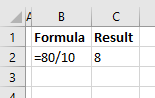
The divide symbol in Excel is the forward slash on the keyboard (/). This is the same as using the division sign (÷) in mathematics. When you divide two numbers in Excel, start with an equal sign (=), which will create a formula. Then type in the first number (the number you want to divide), followed by the forward slash, and then the number you wish to divide by.
=80/10The result of this formula would then be 8.
Divide With a Cell Reference and a Constant
For greater flexibility in your formula, use the reference of a cell as the number to be divided and a constant as the number to divide by.
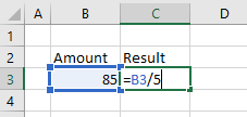
To divide B3 by 5, type the formula:
=B3/5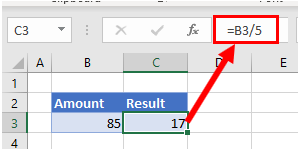
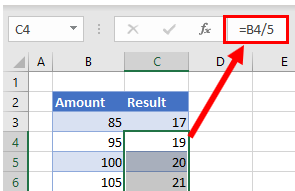
Then copy this formula down the column to the rows below. The constant number (5) will remain the same but the cell address for each row will change according to the row you are in due to Relative Cell referencing.
Divide a Column With Cell References
You can also use a cell reference for the number to divide by.
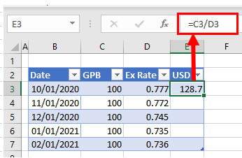
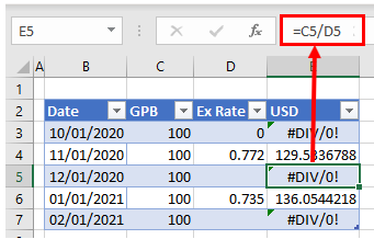
To divide cell C3 by cell D3, type the formula:
=C3/D3Since the formula uses cell addresses, you can then copy this formula down to the rest of the rows in the table.
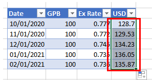
As the formula uses Relative Cell addresses, the formula will change according to the row it is copied down to.
Note: that you can also divide numbers in Excel by using the QUOTIENT Function.
Divide a Column With Paste Special
You can divide a column of numbers by a divisor, and return the result as a number within the same cell.
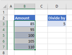
- Select the divisor (in this case, 5) and in the Ribbon, go to Home > Copy, or press CTRL + C.
- Highlight the cells to be divided (in this case B3:B7).
- In the Ribbon, go to Home > Paste > Paste Special.
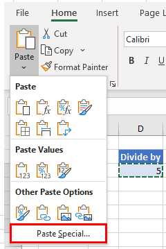
- In the Paste Special dialog box, select Divide and then click OK.
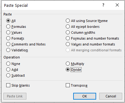
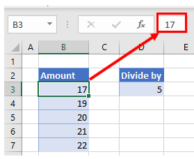
The values in the highlighted cells will be divided by the divisor that was copied and the result will be returned in the same location as the highlighted cells. In other words, you will overwrite your original values with the new divided values; cell references are not used in this this method of calculation.
The #DIV/0! Error
If you try and divide a number by zero, you will get an error as there is no answer when a number is divided by zero.
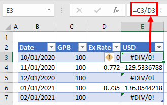
You will also get an error if you try and divide a number by a blank cell.
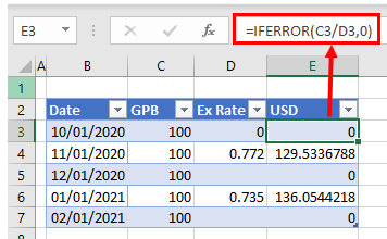
To prevent this from happening, you can use the IFERROR Function in your formula.
Using the methods above, you can also add, subtract, or multiply cells and columns in Excel.
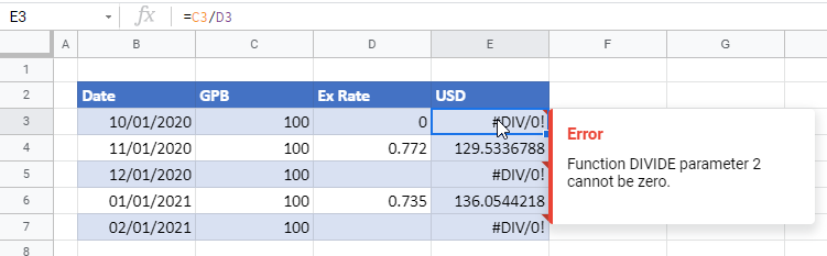
How to Divide Cells and Columns in Google Sheets
Apart from the divide Paste Special function (which does not work in Google Sheets), all of the above examples will work in exactly the same way in Google Sheets.
Содержание
- Split a cell
- Split the content from one cell into two or more cells
- Multiply and divide numbers in Excel
- Multiply numbers
- Multiply numbers in a cell
- Multiply a column of numbers by a constant number
- Multiply numbers in different cells by using a formula
- Divide numbers
- Divide numbers in a cell
- Divide numbers by using cell references
- Distribute the contents of a cell into adjacent columns
- Need more help?
- How to Divide Cells / Columns – Excel & Google Sheets
- The Divide Symbol
- Divide With a Cell Reference and a Constant
- Divide a Column With Cell References
- Divide a Column With Paste Special
- The #DIV/0! Error
- How to Divide Cells and Columns in Google Sheets
- Divide Cell in Excel
- Introduction to Divide Cell in Excel
- Examples of Divide Cell in Excel
- Example #1 – Divide cells with Delimiter in Excel
- Example #2 – Divide cells with Fixed Width in Excel
- Things to Remember
- Recommended Articles
Split a cell
You might want to split a cell into two smaller cells within a single column. Unfortunately, you can’t do this in Excel. Instead, create a new column next to the column that has the cell you want to split and then split the cell. You can also split the contents of a cell into multiple adjacent cells.
See the following screenshots for an example:
Split the content from one cell into two or more cells
Note: Excel for the web doesn’t have the Text to Columns Wizard. Instead, you can Split text into different columns with functions.
Select the cell or cells whose contents you want to split.
Important: When you split the contents, they will overwrite the contents in the next cell to the right, so make sure to have empty space there.
On the Data tab, in the Data Tools group, click Text to Columns. The Convert Text to Columns Wizard opens.
Choose Delimited if it is not already selected, and then click Next.
Select the delimiter or delimiters to define the places where you want to split the cell content. The Data preview section shows you what your content would look like. Click Next.
In the Column data format area, select the data format for the new columns. By default, the columns have the same data format as the original cell. Click Finish.
Источник
Multiply and divide numbers in Excel
Multiplying and dividing in Excel is easy, but you need to create a simple formula to do it. Just remember that all formulas in Excel begin with an equal sign (=), and you can use the formula bar to create them.
Multiply numbers
Let’s say you want to figure out how much bottled water that you need for a customer conference (total attendees × 4 days × 3 bottles per day) or the reimbursement travel cost for a business trip (total miles × 0.46). There are several ways to multiply numbers.
Multiply numbers in a cell
To do this task, use the * (asterisk) arithmetic operator.
For example, if you type =5*10 in a cell, the cell displays the result, 50.
Multiply a column of numbers by a constant number
Suppose you want to multiply each cell in a column of seven numbers by a number that is contained in another cell. In this example, the number you want to multiply by is 3, contained in cell C2.
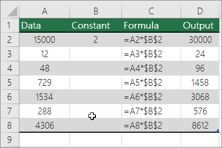
Type =A2*$B$2 in a new column in your spreadsheet (the above example uses column D). Be sure to include a $ symbol before B and before 2 in the formula, and press ENTER.
Note: Using $ symbols tells Excel that the reference to B2 is «absolute,» which means that when you copy the formula to another cell, the reference will always be to cell B2. If you didn’t use $ symbols in the formula and you dragged the formula down to cell B3, Excel would change the formula to =A3*C3, which wouldn’t work, because there is no value in B3.
Drag the formula down to the other cells in the column.
Note: In Excel 2016 for Windows, the cells are populated automatically.
Multiply numbers in different cells by using a formula
You can use the PRODUCT function to multiply numbers, cells, and ranges.
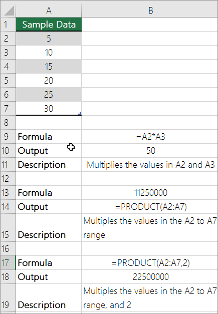
You can use any combination of up to 255 numbers or cell references in the PRODUCT function. For example, the formula =PRODUCT(A2,A4:A15,12,E3:E5,150,G4,H4:J6) multiplies two single cells (A2 and G4), two numbers (12 and 150), and three ranges (A4:A15, E3:E5, and H4:J6).
Divide numbers
Let’s say you want to find out how many person hours it took to finish a project (total project hours ÷ total people on project) or the actual miles per gallon rate for your recent cross-country trip (total miles ÷ total gallons). There are several ways to divide numbers.
Divide numbers in a cell
To do this task, use the / (forward slash) arithmetic operator.
For example, if you type =10/5 in a cell, the cell displays 2.
Important: Be sure to type an equal sign ( =) in the cell before you type the numbers and the / operator; otherwise, Excel will interpret what you type as a date. For example, if you type 7/30, Excel may display 30-Jul in the cell. Or, if you type 12/36, Excel will first convert that value to 12/1/1936 and display 1-Dec in the cell.
Note: There is no DIVIDE function in Excel.
Divide numbers by using cell references
Instead of typing numbers directly in a formula, you can use cell references, such as A2 and A3, to refer to the numbers that you want to divide and divide by.
The example may be easier to understand if you copy it to a blank worksheet.
How to copy an example
Create a blank workbook or worksheet.
Select the example in the Help topic.
Note: Do not select the row or column headers.

Selecting an example from Help
In the worksheet, select cell A1, and press CTRL+V.
To switch between viewing the results and viewing the formulas that return the results, press CTRL+` (grave accent), or on the Formulas tab, click the Show Formulas button.
Источник
Distribute the contents of a cell into adjacent columns
You can divide the contents of a cell and distribute the constituent parts into multiple adjacent cells. For example, if your worksheet contains a column Full Name, you can split that column into two columns—a First Name column and Last Name column.
For an alternative method of distributing text across columns, see the article, Split text among columns by using functions.
You can combine cells with the CONCAT function or the CONCATENATE function.
Follow these steps:
Note: A range containing a column that you want to split can include any number of rows, but it can include no more than one column. It’s important to keep enough blank columns to the right of the selected column, which will prevent data in any adjacent columns from being overwritten by the data that is to be distributed. If necessary, insert a number of empty columns that will be sufficient to contain each of the constituent parts of the distributed data.
Select the cell, range, or entire column that contains the text values that you want to split.
On the Data tab, in the Data Tools group, click Text to Columns.
Follow the instructions in the Convert Text to Columns Wizard to specify how you want to divide the text into separate columns.
Note: For help with completing all the steps of the wizard, see the topic, Split text into different columns with the Convert Text to Columns Wizard, or click Help  in the Convert to Text Columns Wizard.
This feature isn’t available in Excel for the web.
If you have the Excel desktop application, you can use the Open in Excel button to open the workbook and distribute the contents of a cell into adjacent columns.
Need more help?
You can always ask an expert in the Excel Tech Community or get support in the Answers community.
Источник
How to Divide Cells / Columns – Excel & Google Sheets
This tutorial will demonstrate how to divide cells and columns in Excel and Google Sheets.
The Divide Symbol
The divide symbol in Excel is the forward slash on the keyboard (/). This is the same as using the division sign (÷) in mathematics. When you divide two numbers in Excel, start with an equal sign (=), which will create a formula. Then type in the first number (the number you want to divide), followed by the forward slash, and then the number you wish to divide by.
The result of this formula would then be 8.
Divide With a Cell Reference and a Constant
For greater flexibility in your formula, use the reference of a cell as the number to be divided and a constant as the number to divide by.
To divide B3 by 5, type the formula:
Then copy this formula down the column to the rows below. The constant number (5) will remain the same but the cell address for each row will change according to the row you are in due to Relative Cell referencing.
Divide a Column With Cell References
You can also use a cell reference for the number to divide by.
To divide cell C3 by cell D3, type the formula:
Since the formula uses cell addresses, you can then copy this formula down to the rest of the rows in the table.
As the formula uses Relative Cell addresses, the formula will change according to the row it is copied down to.
Note: that you can also divide numbers in Excel by using the QUOTIENT Function.
Divide a Column With Paste Special
You can divide a column of numbers by a divisor, and return the result as a number within the same cell.
- Select the divisor (in this case, 5) and in the Ribbon, go to Home > Copy, or press CTRL + C.
- Highlight the cells to be divided (in this case B3:B7).
- In the Ribbon, go to Home > Paste > Paste Special.
- In the Paste Special dialog box, select Divide and then click OK.
The values in the highlighted cells will be divided by the divisor that was copied and the result will be returned in the same location as the highlighted cells. In other words, you will overwrite your original values with the new divided values; cell references are not used in this this method of calculation.
The #DIV/0! Error
If you try and divide a number by zero, you will get an error as there is no answer when a number is divided by zero.
You will also get an error if you try and divide a number by a blank cell.
![]()
To prevent this from happening, you can use the IFERROR Function in your formula.
Using the methods above, you can also add, subtract, or multiply cells and columns in Excel.
How to Divide Cells and Columns in Google Sheets
Apart from the divide Paste Special function (which does not work in Google Sheets), all of the above examples will work in exactly the same way in Google Sheets.
Источник
Divide Cell in Excel
Excel Divide Cell (Table of Contents)
Introduction to Divide Cell in Excel
When we work with the text files in excel, it has all the data in the single row itself instead of having it in different columns. The data, most of the times, is aligned in a single row with some delimiter or separator in it (such as comma, space, etc.). If you open such files in Excel, you’ll not get the data populated across columns for different attributes, which is a problem in its own ways. It makes dividing the cells into different columns extremely important, and that is exactly what we will walk you through in this article.
Excel functions, formula, charts, formatting creating excel dashboard & others
Data Structure in a Text File:
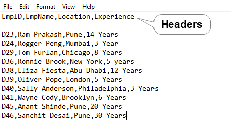
The data is comma-separated if you see the below screenshot and has the first row as column headers. Below that, there is one blank row and then the data values that are comma-separated as well. This type of data is called as delimited data or data with delimiters (in this case, comma as a delimiter).
Let us see the other data set which we are going to use.

This data set simply consists of EmpID and EmpName, as it seems, and there is no special delimiter in this data as well. For both of these types of data, we need to divide the cells into different columns.
Excel has a Text to Column tool, which helps us divide the cells into different columns.
Examples of Divide Cell in Excel
We will see how it works with two examples in this article.
Example #1 – Divide cells with Delimiter in Excel
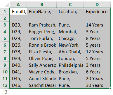
See the data below. The same text file is opened with Excel, which we have seen through the above screenshots and has comma-separated values in it within a single row of the sheet.
To divide it into different columns per field value, we need to use the Text to Column utility in Excel.
Step 1: Select all the cells from column A (spread across the cells A1 to A12) containing data which is comma-separated.
Step 2: Navigate to the Data tab under the Excel ribbon, which is placed at the uppermost corner of the worksheet and click on it.
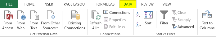
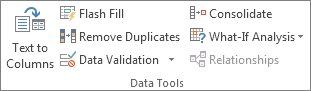
Step 3: As soon as you click on the Data tab, you’ll see different options associated with the data using which we can manipulate the data in Excel. However, you need to navigate to the Data Tools group, under which you’ll see Text to Column as an option.
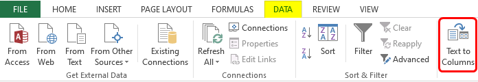
As soon as you click on the Text to Column option, you’ll see Convert Text to Column Wizard popping up on your excel screen, as shown below:
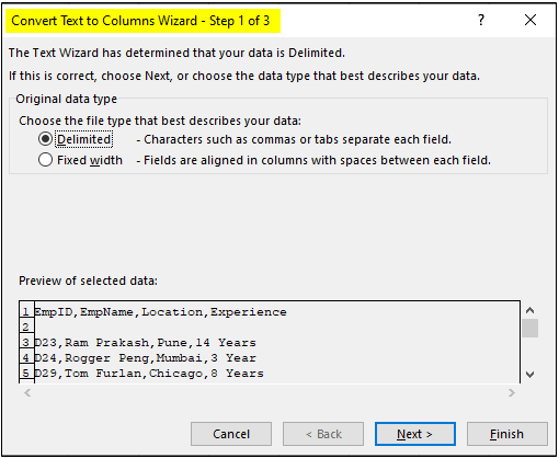
By default, the Delimited option is checked for you. Since our data has a delimiter (comma), we will go with the same selection. Click on the Next > button.
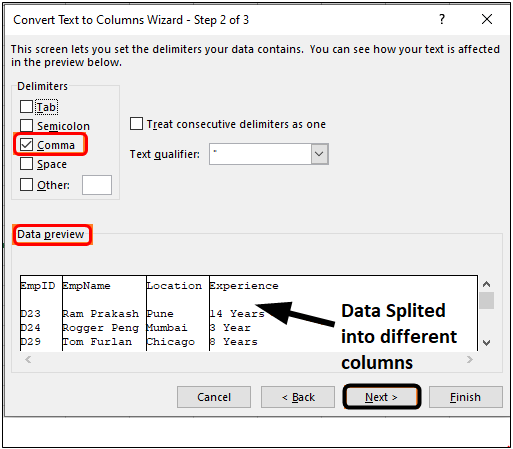
Step 4: Under the Delimiters section, tick the select Comma option (since we have comma-separated data with us). You have different delimiter options such as Tab, Semicolon, Space, etc.; if your data has any delimiter apart from these standard ones, you can use other options to add it as a delimiter for the data to be divided. Since we have a comma with us, we will use the comma as a delimiter. Once you click on the comma, you can see the cell values are divided into separate columns after each comma under the Data preview section. Click on the Next button after done.
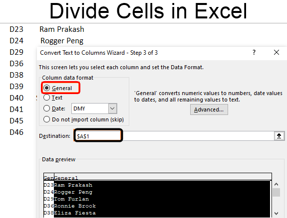
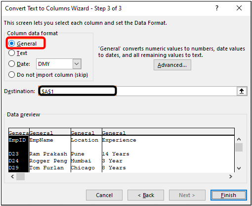
Once you click on the next option, you’ve several options that will allow you to either change the column data type for various columns the data gets split in. Ex. Whether you wanted to store any specific column as a Text or Date format or choose not to import that column with the option, do not import the column (skip) option. Well, these are the options; right now, we are not going to use to and just will use the standard Text to Column settings, in which the Column Data Format is set as General.
Step 5: Set the Column data format as General by clicking the General radio button. Under the Destination: section set the destination as cell A1 and click on the Finish option to complete the dividing data into cells procedure.
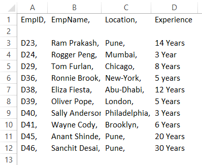
Once you click on the Finish option, you can see data divided across different columns, as shown in the screenshot below:
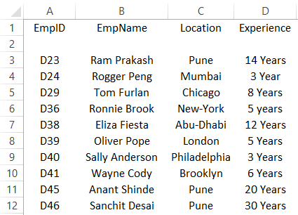
You can see the data which was in a single cell with a comma as a separator or delimiter is now populated across the different columns such as EmpID (column A), EmpName (column B), Location (column C) and Experience (column D).
This is one way to divide cells in Excel when you have delimited data.
Example #2 – Divide cells with Fixed Width in Excel
The Other example is something where you don’t have any delimiter but a data with fixed with and you need to divide the cells containing that data into different columns.
See the data below:

Step 1: Follow the first three steps from the previous example (Example 1) as it is to be able to open the Text to Column Wizard in Excel, which helps in dividing the cells.
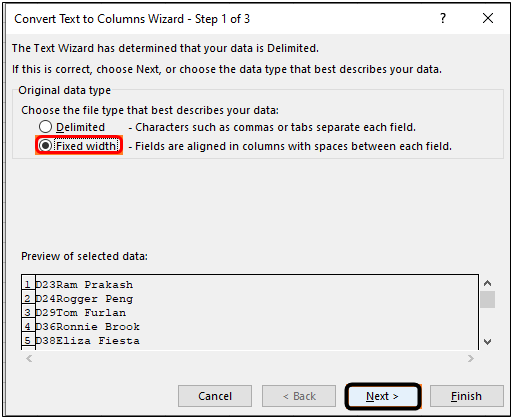
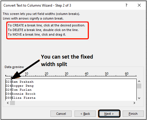
Step 2: Now, as soon as the Convert Text to Columns Wizard gets opened, you need to click the Fixed Width radio button instead of the Delimited (which is set by default). Click on the Next button.
Step 3: After you click on the Next button, you can make the split after a specific length. For Example, we can make a split after the first three characters, which are part of EmpID. See the screenshot below. After you are happy with the split made, click on the Next button.
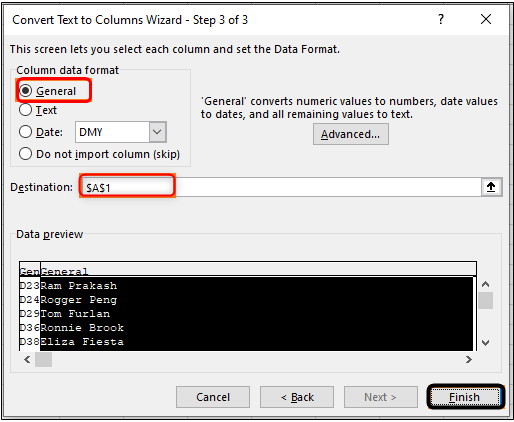
Step 4: On the next screen, you can set the data type as General, Date, etc. And set the Destination Range as well. Once done, you can click on the Finish button. See the screenshot below:
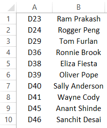
Once you click on the Finish button, you can see the data divided into two different columns, as shown below:
This is how we can divide cells in Excel into different columns using Text to Column wizard.
Things to Remember
- For dividing the cells, your data should have a common delimiter for all the fields. Otherwise, it is not possible to divide the data into different columns.
- If the data doesn’t have a delimiter, you can use the Fixed Width option as well. However, your data should have a fixed number of characters where a split can happen for that to happen. For Ex. after every third character, you may create a split (as shown in Example 2.)
Recommended Articles
This has been a guide to Divide Cell in Excel. Here we discuss How to use Divide Cell in Excel along with practical examples and a downloadable excel template. You can also go through our other suggested articles –
Источник
Excel Divide Cell (Table of Contents)
- Introduction to Divide Cell in Excel
- Examples of Divide Cell in Excel
Introduction to Divide Cell in Excel
When we work with the text files in excel, it has all the data in the single row itself instead of having it in different columns. The data, most of the times, is aligned in a single row with some delimiter or separator in it (such as comma, space, etc.). If you open such files in Excel, you’ll not get the data populated across columns for different attributes, which is a problem in its own ways. It makes dividing the cells into different columns extremely important, and that is exactly what we will walk you through in this article.
Data Structure in a Text File:
The data is comma-separated if you see the below screenshot and has the first row as column headers. Below that, there is one blank row and then the data values that are comma-separated as well. This type of data is called as delimited data or data with delimiters (in this case, comma as a delimiter).
Let us see the other data set which we are going to use.
This data set simply consists of EmpID and EmpName, as it seems, and there is no special delimiter in this data as well. For both of these types of data, we need to divide the cells into different columns.
Excel has a Text to Column tool, which helps us divide the cells into different columns.
Examples of Divide Cell in Excel
We will see how it works with two examples in this article.
Example #1 – Divide cells with Delimiter in Excel
See the data below. The same text file is opened with Excel, which we have seen through the above screenshots and has comma-separated values in it within a single row of the sheet.
To divide it into different columns per field value, we need to use the Text to Column utility in Excel.
Step 1: Select all the cells from column A (spread across the cells A1 to A12) containing data which is comma-separated.
Step 2: Navigate to the Data tab under the Excel ribbon, which is placed at the uppermost corner of the worksheet and click on it.
Step 3: As soon as you click on the Data tab, you’ll see different options associated with the data using which we can manipulate the data in Excel. However, you need to navigate to the Data Tools group, under which you’ll see Text to Column as an option.
As soon as you click on the Text to Column option, you’ll see Convert Text to Column Wizard popping up on your excel screen, as shown below:
By default, the Delimited option is checked for you. Since our data has a delimiter (comma), we will go with the same selection. Click on the Next > button.
Step 4: Under the Delimiters section, tick the select Comma option (since we have comma-separated data with us). You have different delimiter options such as Tab, Semicolon, Space, etc.; if your data has any delimiter apart from these standard ones, you can use other options to add it as a delimiter for the data to be divided. Since we have a comma with us, we will use the comma as a delimiter. Once you click on the comma, you can see the cell values are divided into separate columns after each comma under the Data preview section. Click on the Next button after done.
Once you click on the next option, you’ve several options that will allow you to either change the column data type for various columns the data gets split in. Ex. Whether you wanted to store any specific column as a Text or Date format or choose not to import that column with the option, do not import the column (skip) option. Well, these are the options; right now, we are not going to use to and just will use the standard Text to Column settings, in which the Column Data Format is set as General.
Step 5: Set the Column data format as General by clicking the General radio button. Under the Destination: section set the destination as cell A1 and click on the Finish option to complete the dividing data into cells procedure.
Once you click on the Finish option, you can see data divided across different columns, as shown in the screenshot below:
You can see the data which was in a single cell with a comma as a separator or delimiter is now populated across the different columns such as EmpID (column A), EmpName (column B), Location (column C) and Experience (column D).
This is one way to divide cells in Excel when you have delimited data.
Example #2 – Divide cells with Fixed Width in Excel
The Other example is something where you don’t have any delimiter but a data with fixed with and you need to divide the cells containing that data into different columns.
See the data below:
Step 1: Follow the first three steps from the previous example (Example 1) as it is to be able to open the Text to Column Wizard in Excel, which helps in dividing the cells.
Step 2: Now, as soon as the Convert Text to Columns Wizard gets opened, you need to click the Fixed Width radio button instead of the Delimited (which is set by default). Click on the Next button.
Step 3: After you click on the Next button, you can make the split after a specific length. For Example, we can make a split after the first three characters, which are part of EmpID. See the screenshot below. After you are happy with the split made, click on the Next button.
Step 4: On the next screen, you can set the data type as General, Date, etc. And set the Destination Range as well. Once done, you can click on the Finish button. See the screenshot below:
Once you click on the Finish button, you can see the data divided into two different columns, as shown below:
This is how we can divide cells in Excel into different columns using Text to Column wizard.
Things to Remember
- For dividing the cells, your data should have a common delimiter for all the fields. Otherwise, it is not possible to divide the data into different columns.
- If the data doesn’t have a delimiter, you can use the Fixed Width option as well. However, your data should have a fixed number of characters where a split can happen for that to happen. For Ex. after every third character, you may create a split (as shown in Example 2.)
Recommended Articles
This has been a guide to Divide Cell in Excel. Here we discuss How to use Divide Cell in Excel along with practical examples and a downloadable excel template. You can also go through our other suggested articles –
- Divide in Excel Formula
- Format Cells in Excel
- VBA Cells
- VBA Range Cells