
Содержание
- Статьи из блога
- Подсчет уникальных значений в столбце
- Как работает формула уникальных значений Excel count
- Подсчет уникальных текстовых значений в Excel
- Подсчет уникальных числовых значений в Excel
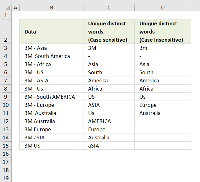
- Подсчет уникальных значений с учетом регистра в Excel
- Подсчитайте различные значения в Excel (уникальные и 1-й повторяющиеся вхождения)
- Как работает формула Excel distinct
- Формулы для подсчета различных значений различных типов
- Подсчитывайте различные значения, игнорируя пустые ячейки
- Формула для подсчета различных текстовых значений
- Формула для подсчета различных чисел
- Подсчет различных значений с учетом регистра в Excel
- Подсчет уникальных и отличных строк в Excel
- Подсчет различных значений в Excel с помощью сводной таблицы
Статьи из блога
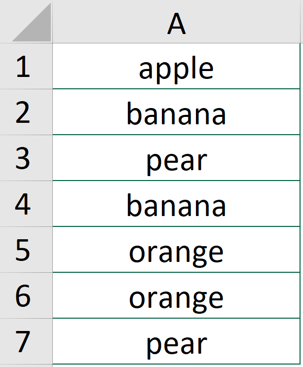
При работе с большим набором данных в Excel часто может потребоваться знать, сколько существует повторяющихся и уникальных значений. И иногда, вы можете считать только различные (разные) значения.
Если вы посещали этот блог на регулярной основе, вы уже знаете формулу Excel для подсчета дубликатов. И сегодня мы собираемся исследовать различные способы подсчета уникальных значений в Excel. Но для большей ясности давайте сначала определимся с терминами.
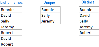
- Уникальные значения-это значения, которые появляются в списке только один раз.
- Различные значения-это все разные значения в списке, т. е. уникальные значения плюс 1 st вхождений повторяющихся значений.
На следующем снимке экрана показана разница:
А теперь давайте посмотрим, как вы можете рассчитывать уникальные и отличные значения в Excel, используя формулы и функции сводной таблицы. В этой статье мы затронем следующие темы:
Как подсчитать уникальные значения в Excel; Подсчет уникальных значений в столбце; Подсчет уникальных текстовых значений; Считайте уникальные числа; Подсчет уникальных значений с учетом регистра; Как подсчитать различные значения в Excel; Подсчитывайте различные значения, игнорируя пустые ячейки; Формула для подсчета различных текстовых значений; Формула для подсчета различных чисел; Подсчет различных значений с учетом регистра; Как подсчитать уникальные и различные строки в Excel; Автоматическое подсчет различных значений в сводной таблице; Как подсчитать уникальные значения в Excel;
Вот общая задача, которую все пользователи Excel должны выполнять один раз в то время. У вас есть список данных, и вам нужно узнать количество уникальных значений в этом списке. Как ты это делаешь? Проще, чем вы можете подумать  ниже вы найдете несколько формул для подсчета уникальных значений различных типов.
Подсчет уникальных значений в столбце
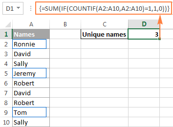
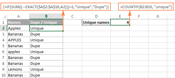
Предположим, у вас есть столбец имен в вашем листе Excel, и вам нужно подсчитать уникальные имена в этом столбце. Решение заключается в использовании функции SUM в сочетании с IF и COUNTIF:
Примечание. Это формула массива, поэтому не забудьте нажать Ctrl + Shift + Enter, чтобы завершить его. Как только вы сделаете это, Excel автоматически заключит формулу в <фигурные скобки>, как на скриншоте ниже. Ни в коем случае не следует вводить фигурные скобки вручную, это не будет работать.
В этом примере мы подсчитываем уникальные имена в диапазоне A2:A10, поэтому наша формула принимает следующую форму:
Подсчет уникальных значений в Excel
Далее в этом уроке мы обсудим несколько других формул для подсчета уникальных значений различных типов. И поскольку все эти формулы являются вариациями базовой формулы уникальных значений Excel, имеет смысл разбить приведенную выше формулу, чтобы вы могли полностью понять, как она работает, и настроить ее для ваших данных. Если кто-то не заинтересован в технических деталях, вы можете сразу перейти к следующему примеру формулы.
Как работает формула уникальных значений Excel count
Как вы видите, в нашей уникальной формуле значений используются 3 различных функции-SUM, IF и COUNTIF. Глядя изнутри наружу, вот что делает каждая функция:
- Функция COUNTIF подсчитывает, сколько раз каждое отдельное значение появляется в указанном диапазоне. В этом примере COUNTIF(A2:A10,A2:A10) возвращает массив <1;2;2;1;2;2;2;1;2>.
- Функция IF оценивает каждое значение в массиве, возвращаемом COUNTIF, сохраняет все 1 (уникальные значения) и заменяет все другие значения нулями. Таким образом, функция IF(COUNTIF(A2:A10,A2:A10)=1,1,0)становится IF(1;2;2;1;2;2;2;1;2) = 1,1,0,тем, что превращается в массив <1;0;0;1;0;0;0;1;0>, где 1-уникальное значение, а 0-повторяющееся значение.
- Наконец, функция SUM суммирует значения в массиве, возвращаемом IF, и выводит общее количество уникальных значений, что именно то, что мы хотели.
Совет. Чтобы узнать, к чему относится определенная часть формулы уникальных значений Excel, выберите эту часть в строке формул и нажмите клавишу F9.
Подсчет уникальных текстовых значений в Excel
Если ваш список Excel содержит как числовые, так и текстовые значения, и вы хотите считать только уникальные текстовые значения, добавьте функцию ISTEXT в Формулу массива, описанную выше:
Как известно, функция Excel ISTEXT возвращает TRUE, если вычисленное значение является текстом, в противном случае-FALSE. Поскольку звездочка (*) работает как оператор AND в формулах массива , функция IF возвращает 1 только в том случае, если значение является одновременно текстовым и уникальным, 0 в противном случае. А после того, как функция SUM сложит все единицы, вы получите количество уникальных текстовых значений в указанном диапазоне.
Не забудьте нажать Ctrl + Shift + Enter, чтобы правильно ввести формулу массива, и вы получите результат, аналогичный этому:
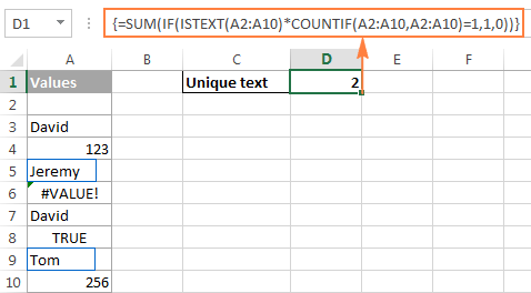
Подсчет уникальных текстовых значений в Excel Как вы можете видеть на скриншоте выше, формула возвращает общее количество уникальных текстовых значений, исключая пустые ячейки, числа, логические значения TRUE и FALSE, а также ошибки.
Подсчет уникальных числовых значений в Excel
Чтобы подсчитать уникальные числа в списке данных, используйте формулу массива, как мы только что использовали для подсчета уникальных текстовых значений, с единственной разницей, что вы вставляете ISNUMBER вместо ISTEXT в свою формулу уникальных значений:
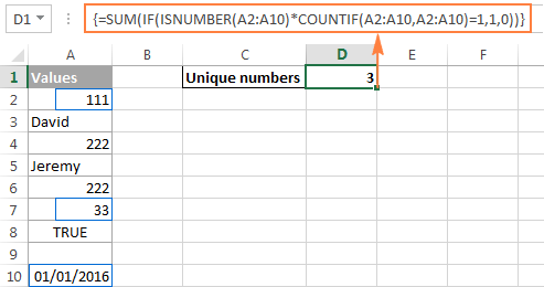
Подсчет уникальных числовых значений в Excel Примечание. Поскольку Microsoft Excel хранит даты и время в виде серийных номеров, они также учитываются.
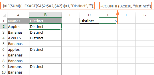
Подсчет уникальных значений с учетом регистра в Excel
Если таблица содержит данные с учетом регистра, самый простой способ подсчета уникальных значений — это создание вспомогательного столбца со следующей формулой массива для идентификации повторяющихся и уникальных элементов:
А затем используйте простую функцию COUNTIF для подсчета уникальных значений:
Подсчет уникальных значений с учетом регистра в Excel
Подсчитайте различные значения в Excel (уникальные и 1-й повторяющиеся вхождения)
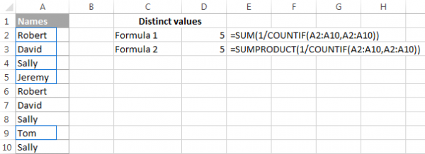
Чтобы получить количество различных значений в списке, используйте следующую формулу:
Помните, что это формула массива, и поэтому вы должны нажать сочетание клавиш Ctrl + Shift + Enter вместо обычного нажатия клавиши Enter.
Кроме того, вы можете использовать функцию SUMPRODUCT и завершить формулу обычным способом, нажав клавишу Enter:
Например, чтобы подсчитать различные значения в диапазоне A2:A10, вы можете пойти с любым из них:
Подсчет различных значений в Excel
Как работает формула Excel distinct
Как вы уже знаете, мы используем функцию COUNTIF, чтобы узнать, сколько раз каждое отдельное значение появляется в указанном диапазоне. В приведенном выше примере результатом функции COUNTIF является следующий массив: <2;2;3;1;2;2;3;1;3>.
После этого выполняется ряд операций деления, где каждое значение массива используется в качестве делителя с 1 в качестве дивиденда. Это превращает все повторяющиеся значения в дробные числа, соответствующие числу повторяющихся вхождений. Например, если значение отображается в списке 2 раза, оно генерирует 2 элемента в массиве со значением 0,5 (1/2=0,5). И если значение появляется 3 раза, он производит 3 элемента в массиве со значением 0.3(3). В нашем примере результатом 1/COUNTIF(A2:A10,A2:A10)) является массив <0.5;0.5;0.3(3);1;0.5;0.5;0.3(3);1;0.3(3)>.
Пока что это не имеет особого смысла? Это потому, что мы еще не применили функцию SUM / SUMPRODUCT. Когда одна из этих функций суммирует значения в массиве, сумма всех дробных чисел для каждого отдельного элемента всегда дает 1, независимо от того, сколько вхождений этого элемента существует в списке. И поскольку все уникальные значения отображаются в массиве как 1 (1/1=1), конечный результат, возвращаемый формулой, является общим числом всех различных значений в списке.
Формулы для подсчета различных значений различных типов
Как и в случае с подсчетом уникальных значений в Excel, можно использовать варианты базовой формулы Excel count distinct для обработки конкретных типов значений, таких как числа, текст и регистрозависимые значения.
Пожалуйста, помните, что все приведенные ниже формулы являются формулами массива и требуют нажатия клавиш Ctrl + Shift + Enter.
Подсчитывайте различные значения, игнорируя пустые ячейки
Если столбец, в котором требуется подсчитать различные значения, может содержать пустые ячейки, следует добавить функцию IF, которая будет проверять указанный диапазон на наличие пробелов (в этом случае базовая формула Excel distinct, описанная выше, возвращает ошибку #DIV/0):
=SUM(IF(range<>«»,1/COUNTIF(range, range), 0))
Например, для подсчета различных значений в диапазоне A2:A10 используйте следующую формулу массива:
=SUM(IF(A2:A10<>«»,1/COUNTIF(A2:A10, A2:A10), 0))
![]()
Формула для подсчета различных значений игнорирует пустые ячейки
Формула для подсчета различных текстовых значений
Для подсчета различных текстовых значений в столбце мы будем использовать тот же подход, который мы только что использовали для исключения пустых ячеек.
Как вы можете легко догадаться, мы просто встроим функцию ISTEXT в нашу формулу Excel count distinct:
И вот вам реальный пример формулы:
Формула для подсчета различных чисел
Для подсчета различных числовых значений (чисел, дат и времени) используйте функцию ISNUMBER:
Например, чтобы посчитать все различные числа в диапазоне A2:A10, используйте следующую формулу:
Подсчет различных значений с учетом регистра в Excel
Подобно подсчету уникальных значений с учетом регистра, самый простой способ подсчета различных значений с учетом регистра-это добавление вспомогательного столбца с формулой массива, которая идентифицирует уникальные значения, включая первые повторяющиеся вхождения. Формула в основном такая же , как та, которую мы использовали для подсчета уникальных значений с учетом регистра, с одним небольшим изменением в ссылке на ячейку, что делает большую разницу:
Как вы помните, все формулы массива в Excel требуют нажатия клавиш Ctrl + Shift + Enter.
После того, как приведенная выше формула будет завершена, вы можете рассчитывать» отличные » значения с помощью обычной формулы COUNTIF, такой как эта:
Подсчет различных значений с учетом регистра в Excel
Если нет способа добавить вспомогательный столбец на рабочий лист, можно использовать следующую сложную формулу массива для подсчета различных значений с учетом регистра без создания дополнительного столбца:
=SUM(IFERROR(1/IF($A$2:$A$10<>«», FREQUENCY(IF(EXACT($A$2:$A$10, TRANSPOSE($A$2:$A$10)), MATCH(ROW($A$2:$A$10), ROW($A$2:$A$10)), «»), MATCH(ROW($A$2:$A$10), ROW($A$2:$A$10))), 0), 0))
Подсчет уникальных и отличных строк в Excel
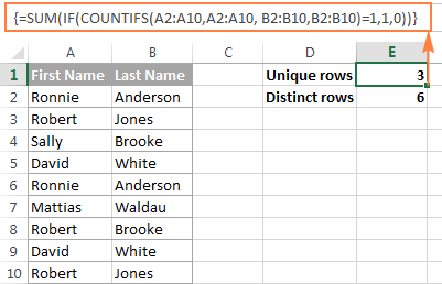
Подсчет уникальных / различных строк в Excel аналогичен подсчету уникальных и различных значений, с той лишь разницей, что вы используете функцию COUNTIFS вместо COUNTIF, которая позволяет указать несколько столбцов для проверки уникальных значений.
Например, для подсчета уникальных или различных имен на основе значений в Столбцах A( имя) и B (фамилия) используйте одну из следующих формул:
Формула для подсчета уникальных строк:
Формула для подсчета различных строк:
Подсчет уникальных и отчетливых строк в Excel
Естественно, вы не ограничены подсчетом уникальных строк, основанных только на двух столбцах, функция COUNTIFS Excel может обрабатывать до 127 пар диапазонов/критериев.
Подсчет различных значений в Excel с помощью сводной таблицы
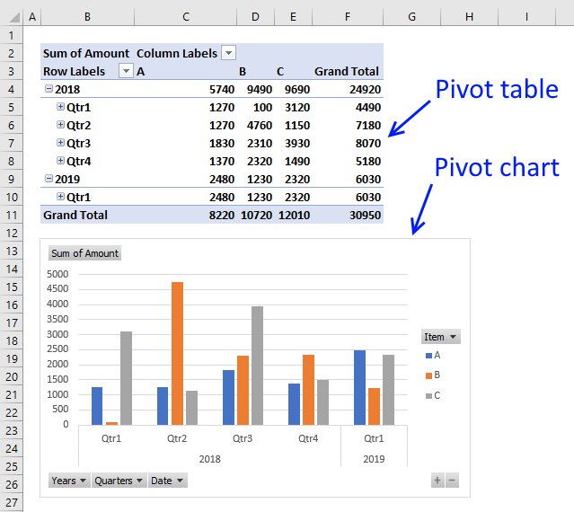
Последние версии Excel 2013 и Excel 2016 имеют специальную функцию, которая позволяет автоматически подсчитывать различные значения в сводной таблице. Следующий снимок экрана дает представление о том, как выглядит Excel Distinct Count:
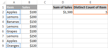
Число различных объектов в сводной таблице
Чтобы создать сводную таблицу с определенным числом различных столбцов, выполните следующие действия.
1. Выберите данные для включения в сводную таблицу, перейдите на вкладку Вставка, группа таблицы и нажмите кнопку Сводная таблица.
2. В диалоговом окне создать сводную таблицу выберите, следует ли разместить сводную таблицу на новом или существующем листе, и обязательно установите флажок добавить эти данные в модель данных.
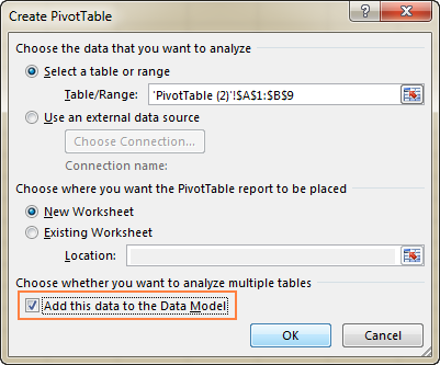
Установите флажок «добавить эти данные в модель данных».
3. Когда ваша сводная таблица откроется, расположите строки, столбцы и области значений так, как вы хотите. Если у вас нет большого опыта работы с сводными таблицами Excel, могут оказаться полезными следующие подробные рекомендации: создание сводной таблицы в Excel.
4. Переместите поле, для которого требуется вычислить число различных объектов (поле элемента в данном примере) , в область значений, щелкните его и в раскрывающемся меню выберите параметры значения поля. :
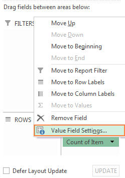
Переместите поле, число различных значений которого вы хотите вычислить, в область значения и выберите параметры значения поля… Откроется диалоговое окно настройки поля значений, вы прокрутите вниз до объекта подсчет различных значений, который является самым последним параметром в списке, выберите его и нажмите кнопку ОК.
Вы также можете задать собственное имя для вашего отдельного счетчика, если хотите.
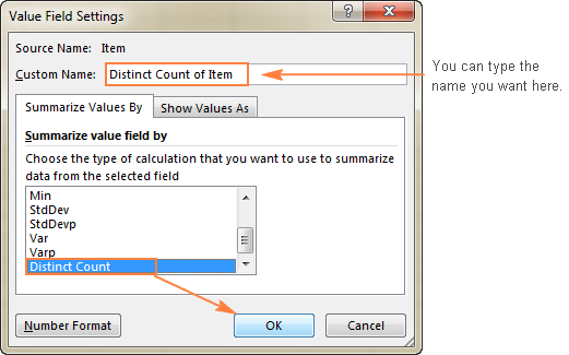
Прокрутите вниз до самого последнего варианта и выберите Distinct Count.
— Готово! Вновь созданная сводная таблица будет отображать отдельный счетчик, как показано на самом первом скриншоте в этом разделе.
Совет. После обновления исходных данных не забудьте обновить сводную таблицу, чтобы обновить число различных объектов. Чтобы обновить сводную таблицу, просто нажмите кнопку Обновить на вкладке анализ в группе данных.
Именно так вы считаете различные и уникальные значения в Excel.
Я благодарю вас за чтение и надеюсь увидеть вас снова на следующей неделе. В следующей статье мы обсудим различные способы поиска, фильтрации, извлечения и выделения уникальных значений в Excel . Пожалуйста, оставайтесь с нами!
Источник
Access для Microsoft 365 Access 2021 Access 2019 Access 2016 Access 2013 Access 2010 Access 2007 Еще…Меньше
Свойство UniqueValues можно использовать, если нужно опустить записи, содержащие повторяющиеся данные в полях, отображаемом Режим таблицы. Например, если выходные данные запроса включают несколько полей, сочетание значений из всех полей должно быть уникальным для записи, которая будет включена в результаты.
Примечание: Свойство UniqueValues применяется только к запросам на добавление, создание таблицы и выборку.
Значения
Свойство UniqueValues может принимать следующие значения:
|
Значение |
Описание |
|
Yes (Да) |
Отображаются только записи, содержащие уникальные значения всех полей, отображаемых в режиме таблицы. |
|
No (Нет) |
(По умолчанию.) Отображаются все записи. |
Свойство UniqueValues можно настроить на его окне свойств режим SQL в Окно запроса.
Примечание: Это свойство можно задать при создании запроса с помощью инструкции SQL. Предикат DISTINCT соответствует значению свойства UniqueValues. Предикат DISTINCTROW соответствует значению свойства UniqueRecords.
Замечания
Если для свойства UniqueValues (Уникальные значения) установлено значение Yes (Да), результаты запроса не будут обновляться и отражать последующие изменения, сделанные пользователями.
Свойства UniqueValues и UniqueRecords связаны тем, что только для одного из них одновременно можно установить «Да». Например, если задав для свойства UniqueValues для свойства «Да» Microsoft Office Access 2007 будет автоматически установлено свойство UniqueRecords (Нет). Однако значение No можно указать для обоих этих свойств. Если для обоих свойств задано значение No, возвращаются все записи.
Совет
Если необходимо подсчитать количество экземпляров значения в поле, создайте итоговый запрос.
Пример
Инструкция SELECT в этом примере возвращает список стран и регионов, в которых проживают клиенты. Так как в стране или регионе может быть множество клиентов, соответствующее значение у многих записей в таблице Customers может совпадать. Однако каждая страна или регион в результатах запроса отображается только один раз.
В этом примере используется таблица Customers, включающая следующие данные:
|
Страна или регион |
Название компании |
|
Бразилия |
Familia Arquibaldo |
|
Бразилия |
Gourmet Lanchonetes |
|
Бразилия |
Hanari Carnes |
|
Франция |
Du monde entier |
|
Франция |
Folies gourmandes |
|
Германия |
Frankenversand |
|
Ирландия |
Hungry Owl All-Night Grocers |
Эта инструкция SQL возвращает страны и регионы, перечисленные в таблице:
SELECT DISTINCT Customers.CountryRegion
FROM Customers;
|
Возвращаемые страны и регионы |
|
Бразилия |
|
Франция |
|
Германия |
|
Ирландия |
Нужна дополнительная помощь?
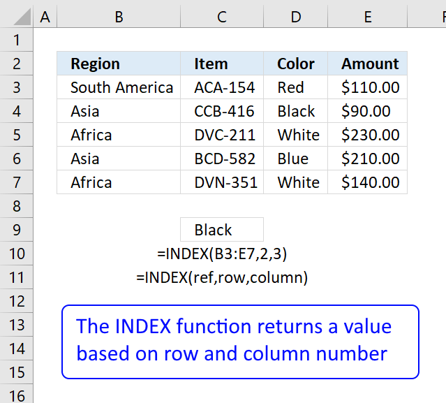
In SQL, SELECT DISTINCT allows us to obtain only unique values from a list. What about Excel select distinct? How can we obtain unique values from a list dynamically with a formula? In this guide, we find out exactly that: a formula in excel to select distinct values dynamically. This guide is updated in 2021, and it simplifies a lot what you have to do with new formulas.
Excel Select Distinct (Quick and Easy, 2021)
Excel Select Distinct Formula (=UNIQUE)
This is the new method we should use, because it is literally just one formula to create our Excel select distinct result. The formula to select distinct values in Excel is Unique.
=UNIQUE(array, [by_col], [exactly_once])
It’s not an array formula in the strict sense, it is just a normal formula that you complete by pressing enter, just like SUM or any other normal formula. The parameters it wants are the following.
- Array – This is the list that contains all the value, out of which we want to extract only distinct or unique value
- by_col – True to select unique values within a column or vertical array (default), false to select unique values within a row or horizontal array
- exactly_once – True to perform an Excel select distinct and return each different value only once, false otherwise.
Now that you know the theory, let’s see it in practice because it is very simple.
Excel Select Distinct Example
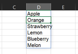
In the A1:A13 range we have a list of fruits, most of which are repeated. We want to extract a list containing each fruit exactly once, removing duplicates with a formula. For that, we resort to =UNIQUE, in its simplest form.
=UNIQUE(A1:A13)
We input this on a cell, D1, and it automatically fills the cells below as needed. This means we need to have enough space below the cells we are entering the UNIQUE formula to host all distinct values, otherwise we will get a #SPILL error.
If you select any cell in the range where you have your formula, you will see a shadow around all the cells that are auto filled with that formula.
To do that, we use the same formula, but we fill the last parameter as TRUE (or simply “1”). To fill the last parameter, we also need to input the optional parameter in the middle, which defaults to true, so we replicate the default value for that by specifying “true” manually.
Excel Select Distinct #SPILL Error
For the UNIQUE function to work and perform an Excel select distinct operation correctly, it needs to have enough space in the cells below it. With enough space, we mean enough space to present all the unique values, so how much space it depends on how much distinct values we have in the original dataset.
If, for some reason, we do not have enough space (we have some content below it), we will get a #SPILL error, meaning that the results would “spill out” of the space that we have available.
If we get the error, instead of displaying as many results as possible, Excel will just present the #SPILL error in the first cell and show no result. This is to prevent that we do some calculation or analysis on incomplete data, with the conviction of having the full set.
By selecting the cell with the #SPILL error we can see a border that shows where the results are to be plotted, so we know how much space we need to make for them.
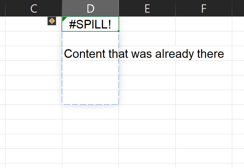
In this case, we can simply remove the previous content and the UNIQUE formula will go ahead and automatically fill the space that we make available. Yet, in other cases you may need to add additional rows or have content you cannot remove, thus you will need to do more advanced work to create the space you need.
Excel Select Distinct (Cumbersome, 2007)
This is the approach that you will find in many other tutorials online because it was the only one available until 2020. It involves an Array formula, a formula that returns multiple values and not just one.
Since this is an array formula, you cannot complete by pressing just Enter like a normal formula, but you complete it by pressing Ctrl + Shift + Enter. Furthermore, you do not select only one cell to see the magic fill the cells below. You have to select all the range where you want your results to appear, then enter the formula and then save it with Ctrl + Shift + Enter.
The idea is this simple: for each cell in the original dataset, we check if we already returned it up until now. If not, we return it, otherwise we just skip it.
For the American version of Excel, use:
=IFERROR(INDEX($A$2:$A$10, MATCH(0, COUNTIF($B$1:B1, $A$2:$A$10), 0)), "")
For the European version of Excel (with semicolons), use:
=IFERROR(INDEX($A$2:$A$10; MATCH(0; COUNTIF($B$1:B1; $A$2:$A$10); 0)); "")
Remember to complete it with Ctrl + Shift + Enter, otherwise it will not work!
In this formula, that we type in cell B2, we have two key parts:
$A$2:$A$10is the range of the original dataset, it must be fixed (with $ sign)$B$1:B1is the range of Excel select distinct values that we have obtained up until now. It starts with B1, which is the header and that must be different from any value in the list, and as we will go down the second part of the range (B1 without dollar sign) will move down to include more and more data, so we are able to check the data that already fetched.
It is crucial that you have a header, and that this header (the first line) contains a value that never appears among the list of values in the original dataset.
Excel Select Distinct in Summary
In short, using Excel to Select Distinct values is extremely easy now that we have the UNIQUE formula. We just need to input our original data set and that’s it. With this knowledge in mind, you can go on creating complex Excels and data models, in a way that is simply unprecedented.
If you want to know how to put your skills to good use in finance, I suggest starting with this ultimate guide on Net Present Value. You may also want to check Microsoft Excel official website.
Author: Oscar Cronquist Article last updated on February 22, 2023

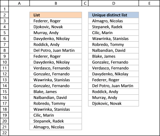
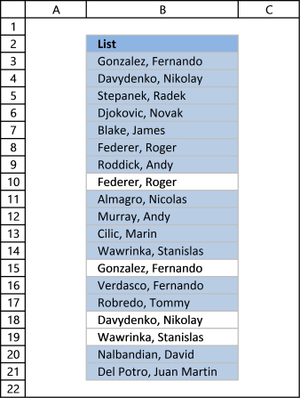
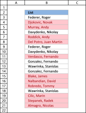
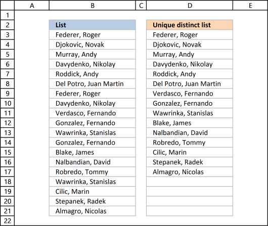
First, let me explain the difference between unique values and unique distinct values, it is important you know the difference so you can find the information you are looking for on this web page.
The picture above shows a list of values in column B, note value AA has a duplicate. Unique distinct values are all cell values but duplicate values are merged into one distinct value. In other words, duplicates are removed only one instance of each value is left in the list.
Column F contains unique values from column B, meaning values that exist only once in column B. Value AA is not in column F because it has a duplicate, in other words, AA is not unique in column B. To filter duplicates, read this post: Extract a list of duplicates from a column
Table of Contents
Working with unique distinct values
- How to extract unique distinct values from a column [Formula]
- Video
- Copy unique distinct values
- Explaining formula
- Get Excel file
- Extract unique distinct values (case sensitive) [Formula]
- Video
- Explaining formula
- Get Excel file
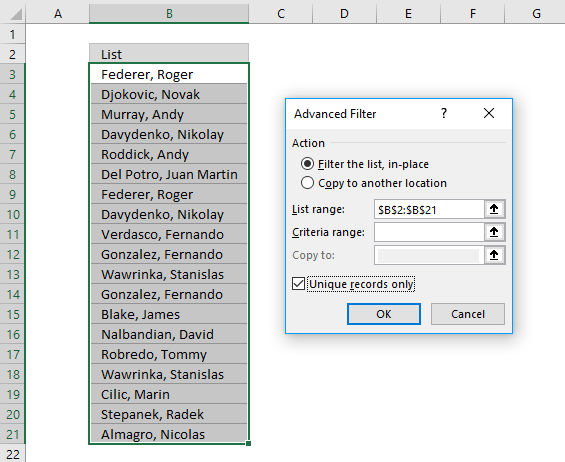
- Filter unique distinct values [Advanced Filter]
- Video
- Copy unique distinct values to another location
- Filter unique distinct values, in place
- Highlight unique distinct values [Conditional Formatting]
- Video
- Explaining formula
- Sort Conditional formatted cells at the top
- How to hide duplicate values [Conditional Formatting]
- Put unique distinct values at the top of the list [Conditional Formatting]
- Extract unique distinct sorted values from a cell range [UDF]
- Video
- How to create an array formula
- VBA code
- Where to put the code?
- Filter unique distinct values from multiple sheets [Add-In]
- Video
- How to extract unique distinct values from a column [Old array Formula]
- How to create an array formula
- Explaining formulaExtract unique distinct values — Pivot Table (Link)
Working with unique values
- How to filter unique values from a list [Formula]
- Explaining formula
- Get Excel file
- Highlight unique values [Conditional Formatting]
- Video
- Sort unique values at the top
- Useful tips
- Excel defined tables
- Named ranges
- Remove errors, Excel version 2007 and later
- Remove errors, Excel version 2003 and earlier
- How to ignore blank cells
- Video
- Get Excel file
- What you will learn in this article
- What is possible with formulas?
- What is the easiest way to filter unique distinct values?
What you will learn in this article
- The difference between unique distinct values and unique values.
- How to decide which Excel feature to use.
- How to use a formula that extracts unique distinct values.
- How to copy the values returned by the formula.
- How the formula works and the functions being used.
- How to filter unique distinct values considering lowercase and uppercase letters.
- How to filter unique distinct values using the Advanced Filter.
- How to highlight unique distinct values using Conditional Formatting.
- How to build a User defined Function that filters unique distinct values sorted from A to Z.
- Where to put the VBA code.
- How to enter and use the User defined Function.
- How to filter unique values using a formula.
- How to highlight unique values using Conditional Formatting.
Back to top
What is possible with formulas?
You have quite a few options to choose from if you are looking for a way to create a unique distinct list in your workbook, all demonstrated in this post or on this website. Not only an exceptionally small regular formula, if you want to use that, but also awesome built-in features in Excel that makes your work so much easier.
Formulas are very versatile, they allow you to build solutions for very specific tasks like filtering unique distinct values from two separate columns or three. If your list contains blanks then this article is for you: Extract a unique distinct list and remove blanks
Perhaps you want to do a wildcard lookup and return unique distinct values or simply return unique distinct values based on a condition.
I have also written articles that explains how to create a unique distinct list sorted alphabetically, sum or frequency.
There is also a formula for extracting unique distinct values located in a multi-column cell range, it is a somewhat more complicated array formula, however, there is a custom function as well, if you prefer that.
Back to top
What is the easiest way to filter unique distinct values?

I would choose the advanced filter if you are not looking for a formula. It lets you quickly filter a unique distinct list.
If you know that you will be extracting unique distinct values from time to time, like in a dashboard or an interactive worksheet, I recommend using a formula and an Excel defined table. You won’t need to repeat the same steps over and over compared to the advanced filter and that will save you time and repetitive work.
However working with a large data set may slow down the formula calculations considerably depending on your computer hardware, so perhaps the User Defined Function [UDF] is a better choice or even better a pivot table, if you have huge amounts of data to work with.
The Excel Pivot table is lightning fast even with huge data tables but it does have a little learning curve and it requires a few steps to set it up but in my opinion, it is totally worth learning how to use pivot tables. You will be surprised how easy it is to start working with Excel Pivot tables.
Conditional Formatting allows you to format cells determined by a built-in rule or a formula you construct. In this post, you will find a Conditional Formatting formula that highlights unique and unique distinct values. Did you know that you can easily sort highlighted values on top? Check out conditional formatting.
I have made an add-in that lets you extract unique, unique distinct and duplicate values and records from multiple worksheets. This allows you to easily bring together data from multiple sources in your workbook.
There is also a useful array formula in this article that extracts a case-sensitive unique distinct list, this is a special case which the built-in Excel tools can’t accomplish.
Back to top
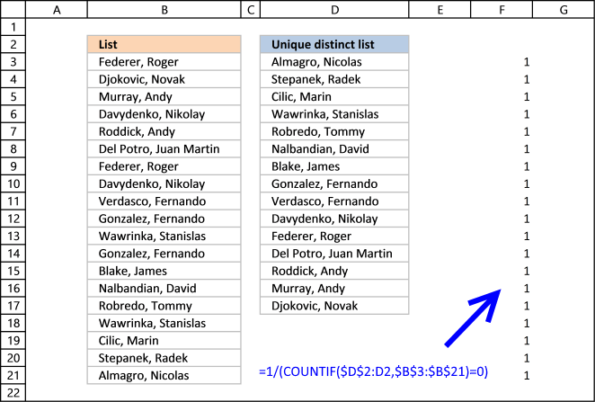
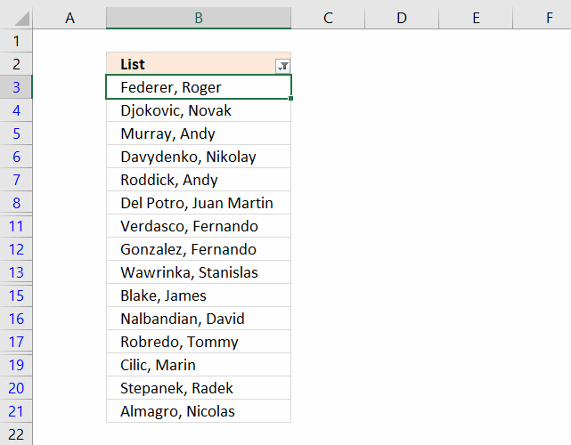
1. Create a list of unique distinct values
Column B contains names, some cells have duplicate values. A formula in column D extracts a unique distinct list from column B.
Update: 2017-08-15!
This formula is even smaller than the array formula and you are not required to enter this as an array formula. The following formula is for older Excel versions than Excel 365 subscribers.
Formula in cell D3:
=LOOKUP(2,1/(COUNTIF($D$2:D2,$B$3:$B$21)=0),$B$3:$B$21)
I will explain how this formula works in the video below and in section 1.3 also below.
Back to top
Update: 2020-05-28!
Microsoft Excel released new functions for Excel 365 subscribers in January 2020. One of those new functions is the UNIQUE function, it allows you to easily extract a unique distinct list using only one function.
Formula in cell D3:
=UNIQUE(B3:B21)
This formula is entered as a regular formula, however, it is a dynamic array formula. Microsoft Excel introduced dynamic array formulas in January 2020 as well.
Dynamic array formulas expand to cells below automatically if more than one value is returned from the formula. Microsoft Excel calls this behavior spilling. You can find more example of the UNIQUE function here.
I will describe a formula for older Excel versions below.
Extract unique distinct values — Excel 365 (Link)
Extract unique distinct values sorted from A to Z — Excel 365 (Link)
Extract unique distinct values ignoring blanks — Excel 365 (Link)
Extract unique distinct values sorted from A to Z ignoring blanks — Excel 365 (Link)
1.1 Video
This video demonstrates how to use the formula:
Subscribe to Get Digital Help on Youtube:
Back to top
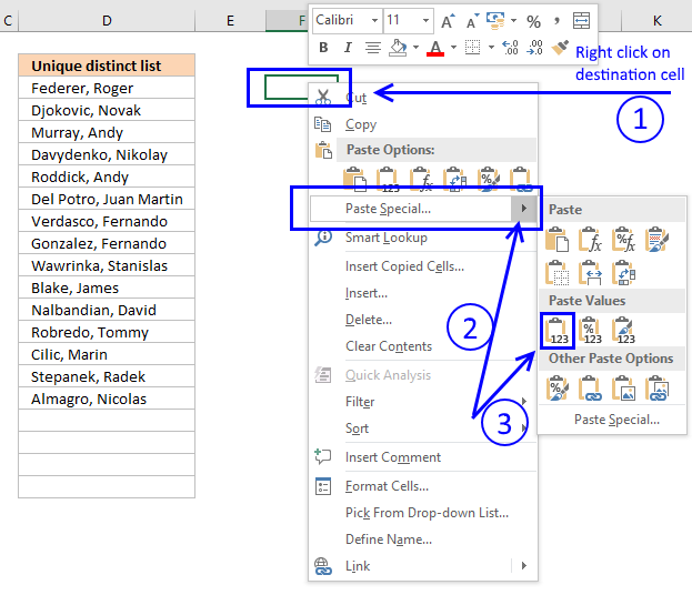
1.2 Copy unique distinct values
To copy unique distinct values to another location you must make sure you copy the values and not the formula:
- Select list
- Copy list, shortcut keys: CTRL + C or press this button:
- Press with right mouse button on on destination cell and press with left mouse button on the black arrow next to «Paste Special…»

- Then press with left mouse button on «Paste Values» button.
Back to top
1.3 Explaining formula in cell D3
Step 1 — Count previous values above the current cell
The COUNTIF function allows you to count values based on a condition. With the help from an expanding cell reference, the formula knows which of the values that have been extracted.
In cell D3 no values have been extracted so it compares the value in the cell above current cell, this happens to be the Header value. Make sure you don’t have a value in the list that matches the header value, it won’t be extracted.
COUNTIF($D$2:D2,$B$3:$B$21) is entered in column F, displayed in the picture below.
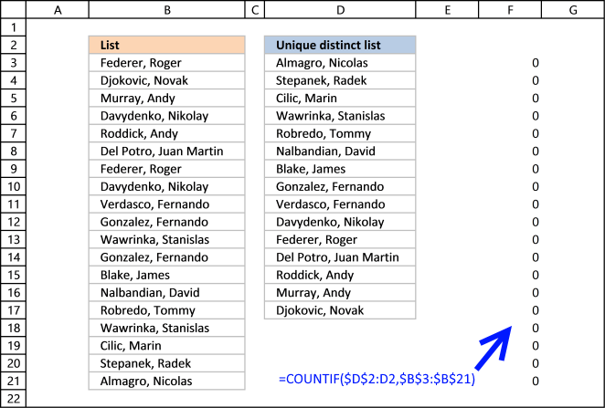
The value in cell D2 is not found in any instance in cell range B3:B21, all values in the array are 0 (zero). Note that the array has the same size as the list in column B, 19 values.
Step 2 — Compare array with 0 (zero)
To identify values that have not been shown the formula compares the array with 0 (zero) and the result are boolean values (TRUE or FALSE) for each value in the array.
COUNTIF($D$2:D2,$B$3:$B$21) = 0
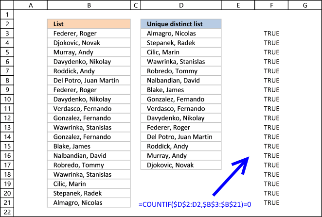
The array contains 19 boolean values, all TRUE.
Step 3 — Divide 1 with array
The boolean value TRUE is equal to 1 and FALSE is equal to 0. If a value in the array is TRUE the result will be 1 because 1/TRUE equals 1.
If a value in the array is FALSE the result will be #DIV0! because 1/FALSE is 1/0 and you can’t divide a number with zero. Excel returns an error.
The good thing about the LOOKUP function is that it ignores errors, see next step.
Step 4 — LOOKUP value
The LOOKUP function is designed to work with sorted cell ranges or arrays, you get weird results if they are not sorted. Be careful using the LOOKUP function.
However, in this case, the values in the array are either 1 or #DIV0!. Surprisingly it ignores errors, the only thing it can find then is a value that is 1.
The first argument in the LOOKUP function is 2 so the function finds the last largest value that is equal to 2 or smaller.
LOOKUP(2,1/(COUNTIF($D$2:D2,$B$3:$B$21)=0),$B$3:$B$21)
becomes
LOOKUP(2,{1;1;1;1;1;1;1;1;1; 1;1;1;1;1;1;1;1;1;1},$B$3:$B$21) and matches the last value in the array. LOOKUP function then returns the corresponding value in cell range $B$3:$B$21 which is Almagro, Nicolas
Back to top
1.4 Excel file
Extract a unique distinct list sorted from A to Z
Extract a unique distinct list sorted from A to Z ignore blanks
Vlookup – Return multiple unique distinct values
Unique distinct list sorted alphabetically based on a condition
Extract a unique distinct list from two columns
Extract a unique distinct list from three columns
Filter unique distinct records
Back to top
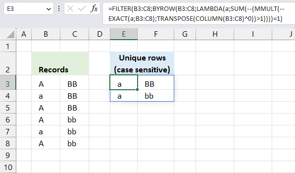
2. Extract a unique distinct list (case sensitive)
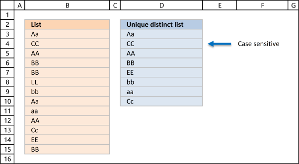
The following array formula lists unique distinct values from a list also considering upper and lower letters. For example, the value «Aa» is not equal to «AA».
Array formula in cell D3:
=INDEX($B$3:$B$15, MATCH(0, FREQUENCY(IF(EXACT($B$3:$B$15, TRANSPOSE($D$2:D2)), MATCH(ROW($B$3:$B$15), ROW($B$3:$B$15)), «»), MATCH(ROW($B$3:$B$15), ROW($B$3:$B$15))), 0))
Excel 365 subscribers can use this regular somewhat shorter formula in cell D3 than the formula below:
=LET(z, B3:B15, x, SEQUENCE(z), INDEX(z, MATCH(0, FREQUENCY(IF(EXACT(z, TRANSPOSE($D$2:D2)), x, «»), x), 0))
The formula above contains two new formulas: LET function and the SEQUENCE function.
This article explains the formula: Extract a case sensitive unique list from a column — Excel 365
2.1 Video
This video demonstrates how to build a formula that extracts a case-sensitive unique distinct list:
Subscribe to Get Digital Help on Youtube:
This post shows you how to extract a case sensitive unique list from a column:
Recommended articles
How to enter an array formula
Back to top
2.2 Explaining the array formula in cell C3
Step 1 — Transpose previous values
TRANSPOSE($D$2:D2)
becomes
TRANSPOSE({«Unique distinct list (case sensitive)»;»Aa»})
and returns
{«Unique distinct list (case sensitive)»,»Aa»}
Note that the ; (semicolon) changes to a , (comma)
Recommended reading:
Recommended articles
Step 2 — Check if two text strings are exactly the same, also case sensitive
EXACT($B$3:$B$15, TRANSPOSE($D$2:D2))
becomes
EXACT($B$3:$B$15, TRANSPOSE({«Unique distinct list (case sensitive)»,»Aa»})
becomes
EXACT($B$3:$B$15, TRANSPOSE({«Unique distinct list (case sensitive)»,»Aa»})
becomes
EXACT({«Aa»; «CC»; «AA»; «BB»; «BB»; «EE»; «bb»; «Aa»; «aa»}, TRANSPOSE({«Unique distinct list (case sensitive)»,»Aa»})
and returns
{FALSE, TRUE; FALSE, FALSE; FALSE, FALSE; FALSE, FALSE; FALSE, FALSE; FALSE, FALSE; FALSE, FALSE; FALSE, TRUE; FALSE, FALSE}
Step 3 — Return relative position in array if TRUE
IF(EXACT($B$3:$B$15, TRANSPOSE($C$1:C1)), MATCH(ROW($B$3:$B$15), ROW($B$3:$B$15))
becomes
IF({FALSE, TRUE; FALSE, FALSE; FALSE, FALSE; FALSE, FALSE; FALSE, FALSE; FALSE, FALSE; FALSE, FALSE; FALSE, TRUE; FALSE, FALSE}, MATCH(ROW($A$1:$A$9), ROW($A$1:$A$9)))
becomes
IF({FALSE, TRUE; FALSE, FALSE; FALSE, FALSE; FALSE, FALSE; FALSE, FALSE; FALSE, FALSE; FALSE, FALSE; FALSE, TRUE; FALSE, FALSE}, {1;2;3;4;5;6;7;8;9})
and returns
{FALSE,1; FALSE,FALSE; FALSE,FALSE; FALSE,FALSE; FALSE,FALSE; FALSE,FALSE; FALSE,FALSE; FALSE,8; FALSE,FALSE}
Recommended article:
Recommended articles

Step 4 — Calculate how often values exist in an array
FREQUENCY(IF(EXACT($B$3:$B$15, TRANSPOSE($C$1:C1)), MATCH(ROW($B$3:$B$15), ROW($B$3:$B$15)), «»), MATCH(ROW($B$3:$B$15), ROW($B$3:$B$15)))
becomes
FREQUENCY({FALSE,1; FALSE,FALSE; FALSE,FALSE; FALSE,FALSE; FALSE,FALSE; FALSE,FALSE; FALSE,FALSE; FALSE,8; FALSE,FALSE},MATCH(ROW($B$3:$B$15),ROW($B$3:$B$15)))
becomes
FREQUENCY({FALSE,1; FALSE,FALSE; FALSE,FALSE; FALSE,FALSE; FALSE,FALSE; FALSE,FALSE; FALSE,FALSE; FALSE,8; FALSE,FALSE},{1;2;3;4;5;6;7;8;9})
and returns
{1;0;0;0;0;0;0;1;0;0} Aa is found in position 1 and 8 in cell range $B$3:$B$15
Recommended articles
Step 5 — Find first empty value (0) in array
MATCH(0, FREQUENCY(IF(EXACT($B$3:$B$15, TRANSPOSE($C$1:C1)), MATCH(ROW($B$3:$B$15), ROW($B$3:$B$15)), «»), MATCH(ROW($B$3:$B$15), ROW($B$3:$B$15))), 0)
becomes
MATCH(0, {1;0;0;0;0;0;0;1;0;0}, 0)
and returns 2.
Recommended articles
Step 6 — Return value from position 2
INDEX($B$3:$B$15, MATCH(0, FREQUENCY(IF(EXACT($B$3:$B$15, TRANSPOSE($C$1:C1)), MATCH(ROW($B$3:$B$15), ROW($B$3:$B$15)), «»), MATCH(ROW($B$3:$B$15), ROW($B$3:$B$15))), 0))
becomes
INDEX($B$3:$B$15, 2)
and returns «CC» in cell C3.
Recommended articles
Back to top
2.3 Excel file
Back to top
Recommended articles
Case sensitive lookup and return multiple values
Filter values based on a condition — case sensitive (Excel 365)
Filter unique distinct values (case sensitive) [UDF]
Filter unique distinct records (case sensitive) [UDF]
Back to top
3. Extract unique distinct values [Advanced Filter]
First a little reminder, unique distinct values are all cell values but duplicate values are merged into one distinct value.

3.1 Video
The following video shows you how to filter unique distinct values using Advanced Filter:
Subscribe to Get Digital Help on Youtube:
Back to top
3.2 Instructions — Copy unique distinct values to another location

This section describes how to extract unique distinct values using the built-in feature «Advanced Filter».
- Go to tab «Data» on the ribbon.
- Press the «Advanced Filter» button on the ribbon.

- Press button «Copy to another location».

- Press «List range:» and select range to filter unique distinct values.
- Press «Copy to: and select a range.
- Press «Unique records only» button to select it.
- Press with left mouse button on «OK» button to apply settings and start extracting.


Back to top
3.3 Instructions — Filter unique distinct values, in place
If you choose to filter unique distinct values in-place, press with left mouse button on the first option button in the dialog box.
You can then select unique distinct values and paste to another location, duplicate values are hidden and are ignored when you copy cell range B3:21 and paste to a new location, very useful.
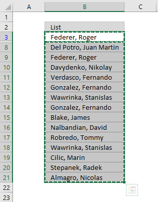
The picture below shows you the selected distinct values after I cleared the Advanced Filter, duplicate values are not selected because they were hidden.
Recommended articles
Lookup and return multiple values [Advanced Filter]
Extract all rows that meet critera in one column [Advanced Filter]
An Advanced Filter is not the only powerful built-in feature in Excel, I highly recommend that you learn pivot tables. Perhaps the most powerful tool but also the least known:
Recommended articles
The Excel defined table is also extremely useful, it allows you to quickly sort, filter and manipulate data. Learn that and much more:
Recommended articles
How to use Excel Tables
An Excel table allows you to easily sort, filter and sum values in a data set where values are related.
Back to top
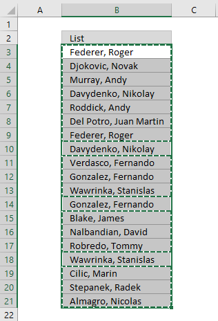
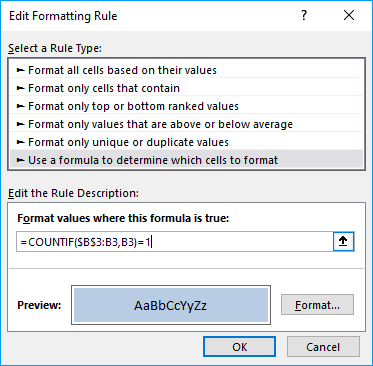
4. Highlight unique distinct values [Conditional Formatting]
This section demonstrates how to highlight unique distinct values using Excel’s built-in feature «Conditional Formatting».
The image shows you unique distinct values highlighted using Conditional Formatting.
4.1 Video
This video demonstrates how to highlight unique distinct values:
Subscribe to Get Digital Help on Youtube:
How to highlight unique distinct values
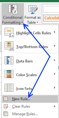
- Select cell range B3:B21.
- Go to tab «Home» on the ribbon.
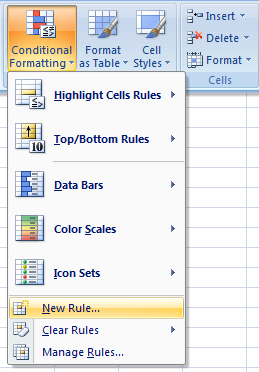
- Press on «Conditional Formatting» button.

- Press on «New Rule…».

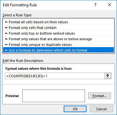
- Press on «Use a formula to determine which cells to format:».
- Type this formula: =COUNTIF($B$3:B3,B3)=1
- Press on «Format…» button.
- Pick a color.
- Press OK button.
- Press OK button again.
Back to top
4.2 Explaining Conditional Formatting formula

A CF formula works somewhat differently than a regular formula, however, they may be harder to spot.
It is possible that you can’t even see if a cell range has CF applied to it or not, if no cells are highlighted.
I recommend that you copy the CF formula and enter it to an adjacent column to better show how they work.
Step 1 — COUNTIF function
The COUNTIF function has two arguments, the first argument is the cell range you want to count a specific value in. The second argument is the value you want to count.
COUNTIF(range, criteria)
Step 2 — COUNTIF arguments
The first argument uses both relative and absolute cell references, $B$3:B3. The absolute part has dollar signs $B$3 meaning it does not change when the Conditional Formatting formula is applied to the next cell.
The relative part B3 does change when the Conditional Formatting formula is applied to the next cell.
COUNTIF($B$3:B3, B3)
Step 3 — Demonstrate calculations in cells B3 and B4
In cell B3 the function is COUNTIF($B$3:B3,B3)
and in cell B4: COUNTIF($B$3:B4,B4) and so on.
This technique using growing cell references lets you highlight the first instance of a value but not duplicate values.
Step 4 — Compare output to 1
How do we know if the value is a unique distinct value? Compare COUNTIF($B$3:B3,B3) to 1 and it will return TRUE or FALSE, like this:
COUNTIF($B$3:B3,B3)=1
The equal sign is a logical operator that returns TRUE or FALSE. Note, the comparison is not case sensitive. The output is a boolean value TRUE or FALSE.
COUNTIF($B$3:B3,B3)=1
becomes
1=1
and returns boolean value TRUE. Cell B3 is highlighted.
If COUNTIF($B$3:B3,B3) returns a number larger than 1 meaning there is at least a duplicate value in the cell range specified in the first argument. That prevents the Conditional Formatting formula from highlighting the cell.
Recommended articles
Highlight unique/duplicates
Highlight current date
Highlight lookup values
Highlight cells equal to
4.3 Sort Conditional formatted cells at the top
Tip! Press with right mouse button on on a highlighted cell, press with left mouse button on Sort and then on «Put Selected Cell Color On top» to arrange unique distinct values at the very top of your list.
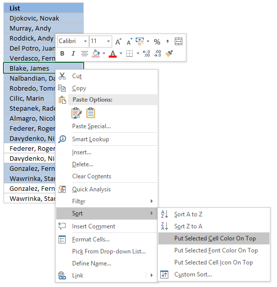
The picture below shows you all unique distinct values sorted together.
Back to top
5. Hide duplicate values [Conditional Formatting]
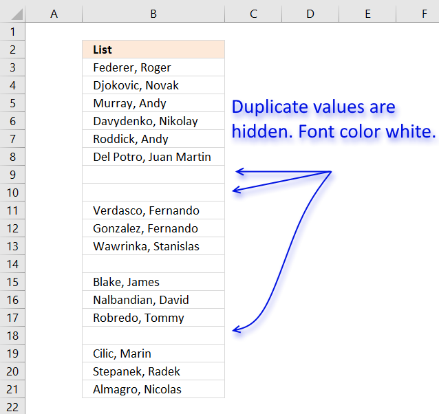
The image above demonstrates Conditional Formatting applied to a list of values, it changes the font color to white for duplicate values making them invisible or they appear hidden.
Keep in mind that the text is still there so if you copy the range and paste the values to a new range the hidden values are visible again. I recommend that you sort the visible values at the top in order to copy them correctly, instructions below.
Conditional Formatting formula:
=COUNTIF($B$3, B3)>1
Back to top
How to apply conditional formatting formula to cell range B3:B21
- Select cell range B3:B21.
- Go to tab «Home» on the ribbon.
- Press with left mouse button on the «Conditional Formatting» button.
- Press with left mouse button on «New Rule…»

- Press with left mouse button on «Use a formula to determine which cells to format:».
- Type the Conditional Formatting formula in «Format values where this is true:».
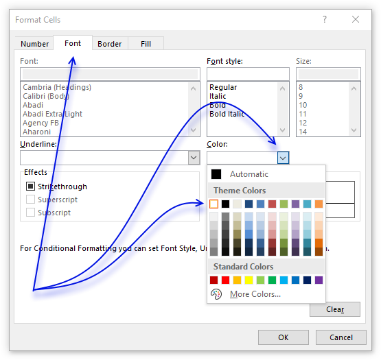
- Press with left mouse button on «Format…» button.

- Go to tab «Font» on the menu, see image above.
- Press with left mouse button on color drop-down list.
- Pick white.
- Press with left mouse button on OK button.
- Press with left mouse button on OK button.
- Press with left mouse button on OK button.
Back to top
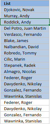
6. How to sort unique distinct values at the top of the list
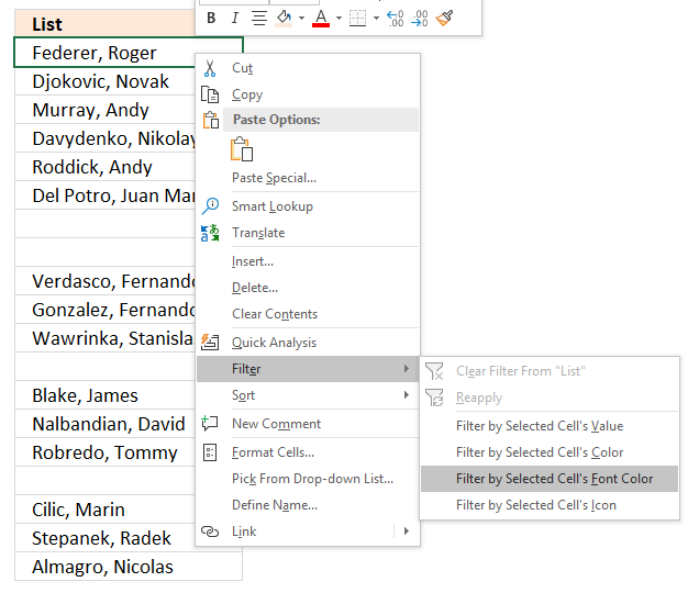
- Press with right mouse button on on one of the visible values in the list.

- Press with left mouse button on «Filter»
- Press with left mouse button on «Filter by Selected Cell’s Font color.
Recommended articles
Highlight unique values and unique distinct values in a multi-column cell range
Highlight unique distinct records
Highlight unique values in a filtered excel table
How to highlight duplicate values in a column
Check out the Conditional formatting category
Back to top
7. Extract unique distinct sorted values from a cell range [UDF]

This UDF lets you create and sort a unique distinct list. First you need to copy the VBA code to your workbook, instructions below. Second, select a cell range. Third, type FilterUniqueSort(cell_ref) in the formula bar. Last, enter formula as an array formula, instructions below.
There is also a workbook for you to get.
Array formula in cell B2:B8212:
=FilterUniqueSort($A$2:$A$8212)
7.1 Video
This video explains how to implement and use the User Defined Function
Subscribe to Get Digital Help on Youtube:
7.2 How to create an array formula
- Type B2:B8212 in name box
- Type above array formula in formula bar

- Press and hold Ctrl + Shift
- Press Enter once
- Release all keys

Recommended reading
Recommended articles

Back to top
7.3 VBA code
I am using the selection sort function to sort values. You can read more about the function here:
Using a Visual Basic Macro to Sort Arrays in Microsoft Excel
'Name User Defined Function and define paremeter
Function FilterUniqueSort(rng As Range)

'Dimension variables and declare data types
Dim ucoll As New Collection, Value As Variant, temp() As Variant
Dim iRows As Single, i As Single

'Redimension array variable
ReDim temp(0)

'Enable error handling
On Error Resume Next

'Iterate through each value in range
For Each Value In rng

'Check if number of characters in value is greater than 0 (zero), if true add value to collection ucoll
If Len(Value) > 0 Then ucoll.Add Value, CStr(Value)

'Continue with next value
Next Value

'Disable error handling
On Error GoTo 0

'Iterate through each value in collection ucoll
For Each Value In ucoll

'Save value to last container in array variable temp
temp(UBound(temp)) = Value

'Add new container to array variable temp
ReDim Preserve temp(UBound(temp) + 1)

'Next value
Next Value

'Remove last container in array variable temp
ReDim Preserve temp(UBound(temp) - 1)

'Save selected rows on worksheet to variable iRows
iRows = Range(Application.Caller.Address).Rows.Count

'Start User Defined Function SelectionSort with values in array variable temp
SelectionSort temp

'Add blanks to array variable temp to prevent error values on worksheet
For i = UBound(temp) To iRows

'Add container
ReDim Preserve temp(UBound(temp) + 1)

'Save blank to container
temp(UBound(temp)) = ""

'Continue with next value
Next i

'Transpose values in array variable temp and return those values to worksheet
FilterUniqueSort = Application.Transpose(temp)

End Function
'Name User Defined Function (UDF) and define parameters
Function SelectionSort(TempArray As Variant)
'This UDF sorts values in an array
'https://www.get-digital-help.com/how-to-extract-a-unique-list-and-the-duplicates-in-excel-from-one-column/#7.3

          'Dimension variables and declare data types
          Dim MaxVal As Variant
          Dim MaxIndex As Integer
          Dim i As Integer, j As Integer

          'Iterate through each value in array variable temp starting from last to first
          For i = UBound(TempArray) To 0 Step -1

              'Save value to variable MaxVal
              MaxVal = TempArray(i)

              'Save value stored in variable i to variable MaxIndex
              MaxIndex = i

              'Iterate through each value in array variable temp
              For j = 0 To i

                  'Check if value in array variable TempArray is larger than value stored in variable MaxVal
                  'Excel can compare text values as well, this action checks if a text value is before or after another value in a sorted list
                  If TempArray(j) > MaxVal Then

                      'If true save value to variable MaxVal
                      MaxVal = TempArray(j)

                      'Save position to MaxIndex
                      MaxIndex = j
                  End If

              'Continue with next value
              Next j

              'Check if number stored in variable MaxIndex is smaller than number stored in variable i
              If MaxIndex < i Then

                  'Save value in array variable TempArray position i to array variable TempArray container position MaxIndex
                  TempArray(MaxIndex) = TempArray(i)

                  'Save value in variable MaxVal to array variable TempArray container position i
                  TempArray(i) = MaxVal
              End If
          Next i

      End Function
Back to top
7.4 Where to copy VBA code?
- Press Alt + F11 to open VB Editor
- Press with left mouse button on «Insert» on the menu
- Press with left mouse button on «Module» to create a module
- Copy (Ctrl + c) above VBA code and paste (Ctrl +v) to the code module
Back to top
More powerful User Defined Functions
Recommended articles
Recommended articles
Recommended articles
Back to top
8. Filter unique distinct values from multiple sheets add-in
Filter unique distinct values is an add-in for Excel 2007/2010/2013 that lets you extract
- unique distinct values
- duplicate values
- unique distinct records
- duplicate records
from multiple sheets. The Add-In contains 4 user-defined functions.
If a value in one of the ranges changes the function will automatically and instantly update the list.
Features
- All user-defined functions remove blank values and blank records.
- No error values when all values are extracted.
- Filter values or records from up to 255 different cell ranges or sheets.
8.1 Watch this video where I demonstrate the Excel Add-In
Subscribe to Get Digital Help on Youtube:
What are unique distinct values?

What are unique distinct records?

Purchase Filter Unique Distinct Values From Multiple Sheets Add-in For Excel 2007/2010/2013 — Price $19 USD
Questions
Is there a money back guarantee?
Sure, you have a unconditional money back guarantee for 14 days.
Back to top
9. Create a list of unique distinct values [Old array Formula]
I recommend using the regular formula above since it is smaller and has an advantage of not being an array formula.
Array formula in cell D3:
=INDEX($B$3:$B$21, MATCH(0, COUNTIF($D$2:D2, $B$3:$B$21), 0))
Thanks to Eero, who contributed the original array formula!
Back to top
The formulas above has an issue with blank cells, it returns a 0 (zero) in your list. This article shows you how to ignore blanks:
Recommended articles
![]()
9.1 How to create an array formula
You don’t need to follow these steps if you chose the regular formula.
- Copy the array formula above (Ctrl + c)
- Double press with left mouse button on cell B2
- Paste (Ctrl + v)
- Press and hold Ctrl + Shift simultaneously
- Press Enter
- Release all keys
If you made the above steps correctly the formula now has a beginning and ending curly bracket, like this:
{=INDEX($B$3:$B$21, MATCH(0, $D$2:D2, $B$3:$B$21), 0))}
Don’t enter these characters yourself, they appear automatically.
Copy cell B2 and paste to cells below as far as needed.
Back to top
9.2 How the array formula in cell B2 works
Step 1 — Create an array with the same size as the list
The COUNTIF function calculates the number of cells equal to a condition.
COUNTIF(range, criteria)
COUNTIF($B$1:B1, $A$2:$A$20)
becomes
COUNTIF(«Unique distinct list»,{Federer,Roger; Djokovic,Novak; Murray,Andy; Davydenko,Nikolay; Roddick,Andy; DelPotro,JuanMartin; Federer,Roger; Davydenko,Nikolay; Verdasco,Fernando; Gonzalez,Fernando; Wawrinka,Stanislas; Gonzalez,Fernando; Blake,James; Nalbandian,David; Robredo,Tommy; Wawrinka,Stanislas; Cilic,Marin; Stepanek,Radek; Almagro,Nicolas} )
and returns:
{0;0;0;0;0;0;0;0;0;0;0;0;0;0;0;0;0;0;0}
This means the cell value in $B$1:B1 can’t be found in any of the cells in cell range $A$2:$A$20. If it had been found, somewhere in the array the number 1 would exist.
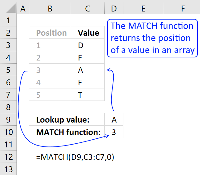
Step 2 — Return the position of an item that matches 0 (zero)
The MATCH function returns the relative position of an item in an array that matches a specified value.
MATCH(lookup_value, lookup_array, [match_type]
MATCH(0, COUNTIF($B$1:B1, $A$2:$A$20), 0)
becomes
MATCH(0,{0; 0; 0; 0; 0; 0; 0; 0; 0; 0; 0; 0; 0; 0; 0; 0; 0; 0; 0},0)
and returns 1.
Step 3 — Return a cell value
The INDEX function returns a value or reference of the cell at the intersection of a particular row and column, in a given range.
INDEX(array, row_num, [column_num])
INDEX($B$3:$B$21, 1)
becomes
=INDEX({Federer,Roger; Djokovic,Novak; Murray,Andy; Davydenko,Nikolay; Roddick,Andy; DelPotro,JuanMartin; Federer,Roger; Davydenko,Nikolay; Verdasco,Fernando; Gonzalez,Fernando; Wawrinka,Stanislas; Gonzalez,Fernando; Blake,James; Nalbandian,David; Robredo,Tommy; Wawrinka,Stanislas; Cilic,Marin; Stepanek,Radek; Almagro,Nicolas}, 1)
and returns «Federer, Roger».
Relative and absolute cell references
When you copy the array formula down the countif formula range ($B$1:B1) expands. This is created by using relative and absolute references.
The first cell, B2: COUNTIF($B$1:B1,$A$2:$A$20)
Second cell, B3: COUNTIF($B$1:B2,$A$2:$A$20)
and so on.
Recommended reading:
Recommended articles
Back to top
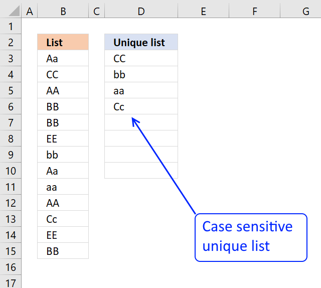
10. How to filter unique values from a list

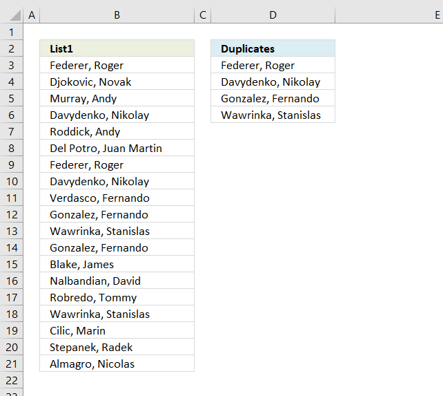
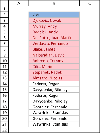
Unique values are values existing only once in a list. Example, «AA» exists twice in the list below and is not unique. BB and CC exist only once each and are unique in the list.
Column D in the picture below filters all unique values from column B. Unique values are values that exist only once in column B.

Example, Roger, Federer is not in column D because there is more than one value of this name in column A. In other words, the name is not unique in column A. You can find the name twice in the list, in cells A2 and A8.
Update 2017-08-30
This formula is even smaller than the array formula and you are not required to enter this as an array formula.
Regular formula in cell D3:
=LOOKUP(2, 1/((COUNTIF(D2:$D$2, $B$3:$B$21)=0)*(COUNTIF($B$3:$B$21, $B$3:$B$21)=1)), $B$3:$B$21)
Recommended articles
How to extract a case sensitive unique list from a column
Filter unique values sorted from A to Z
Extract unique values from two columns
Update 2020-12-09, the formula below extracts unique values from cell range $B$3:$B$21:
Regular formula in cell D3:
=UNIQUE($B$3:$B$21,,TRUE)
The formula above contains the new UNIQUE function that only Excel 365 subscribers can use. Use the formula above if you have an earlier Excel version.
Recommended articles
Extract unique values — Excel 365 (Link)
Extract unique values sorted from A to Z — Excel 365 (Link)
Extract unique values ignoring blanks — Excel 365 (Link)
Extract unique values sorted from A to Z ignoring blanks — Excel 365 (Link)
Array formula in cell D3:
=INDEX($B$3:$B$21, MATCH(0, COUNTIF(D2:$D$2, $B$3:$B$21)+(COUNTIF($B$3:$B$21, $B$3:$B$21)<>1), 0))
How to enter an array formula
Back to top
10.1 Explaining array formula in cell D3
Step 1 — Count each value in array and check if it is not equal to one
(COUNTIF($A$2:$A$20, $A$2:$A$20)<>1
becomes
{2;1;1;2;1;1;2;2;1;2;2;2;1;1;1;2;1;1;1}<>1
and returns
{TRUE; FALSE; FALSE; TRUE; FALSE; FALSE; TRUE; TRUE; FALSE; TRUE; TRUE; TRUE; FALSE; FALSE; FALSE; TRUE; FALSE; FALSE; FALSE}
This array tells excel that the first value in the array is not unique and that is true because Roger, Federer is not unique in the list. However the second value is FALSE and that value is unique, etc.
Recommended articles
Step 2 — Keep track of previous values
C1:$C$1 is a dynamic cell reference, it changes as the formula is copied to cells below. You can read more about absolute and relative cell references here:
Recommended articles
COUNTIF(C1:$C$1, $A$2:$A$20)
becomes
COUNTIF(«Unique list», {«Federer, Roger «; «Djokovic, Novak «; «Murray, Andy «; «Davydenko, Nikolay «; «Roddick, Andy «; «Del Potro, Juan Martin «; «Federer, Roger «; «Davydenko, Nikolay «; «Verdasco, Fernando «; «Gonzalez, Fernando «; «Wawrinka, Stanislas «; «Gonzalez, Fernando «; «Blake, James «; «Nalbandian, David «; «Robredo, Tommy «; «Wawrinka, Stanislas «; «Cilic, Marin «; «Stepanek, Radek «; «Almagro, Nicolas «})
and returns
{0; 0; 0; 0; 0; 0; 0; 0; 0; 0; 0; 0; 0; 0; 0; 0; 0; 0; 0}
A zero (0) means that no values have yet been displayed and that is true in cell C2. However when excel calculates the value in cell C3, cell C2 shows «Djokovic, Novak» and the array becomes {0; 1; 0; 0; 0; 0; 0; 0; 0; 0; 0; 0; 0; 0; 0; 0; 0; 0; 0}. The second value in the array contains 1. This tells excel that value has already been shown.
Step 3 — Add arrays
COUNTIF(C1:$C$1, $A$2:$A$20)+(COUNTIF($A$2:$A$20, $A$2:$A$20)<>1
becomes
{TRUE; FALSE; FALSE; TRUE; FALSE; FALSE; TRUE; TRUE; FALSE; TRUE; TRUE; TRUE; FALSE; FALSE; FALSE; TRUE; FALSE; FALSE; FALSE} + {0; 0; 0; 0; 0; 0; 0; 0; 0; 0; 0; 0; 0; 0; 0; 0; 0; 0; 0}
and returns
{1;0;0;1;0;0;1;1;0;1;1;1;0;0;0;1;0;0;0}
TRUE is 1 and FALSE is zero. So True + 0 equals 1 and False + 1 equals 1.
Step 4 — Find first zero value in array
A zero in the array indicates {1;0;0;1;0;0;1;1;0;1;1;1;0;0;0;1;0;0;0} that the corresponding value is unique and has not yet been displayed in the list.
MATCH(0, COUNTIF(C1:$C$1, $A$2:$A$20)+(COUNTIF($A$2:$A$20, $A$2:$A$20)<>1), 0)
becomes
MATCH(0, {1;0;0;1;0;0;1;1;0;1;1;1;0;0;0;1;0;0;0}, 0)
and returns 2.
Recommended articles
Step 5 — Return corresponding value
INDEX($A$2:$A$20, MATCH(0, COUNTIF(C1:$C$1, $A$2:$A$20)+(COUNTIF($A$2:$A$20, $A$2:$A$20)<>1), 0))
becomes
INDEX($A$2:$A$20, 2)
and returns «Djokovic, Novak» in cell C2.
Recommended articles
Back to top
10.2 Get Excel file
To extract duplicates, see this post:
Recommended articles
Back to top
11. Highlight unique values [Conditional Formatting]
This example demonstrates how to highlight cells with a color of your choice if it contains a unique value.
11.1 Video
The following video shows you how to color unique values using conditional formatting. Remember, it highlights only unique values, in other words, values that exist only once in the list.
Subscribe to Get Digital Help on Youtube:
Instructions
- Go to tab «Home» on the ribbon

- Press with left mouse button on «Conditional Formatting» button
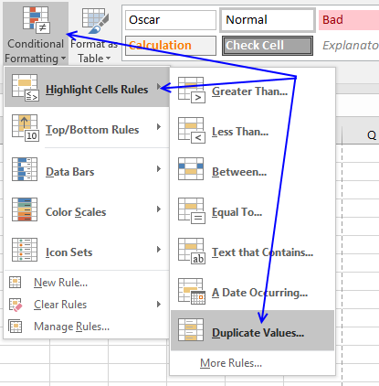
- Hover over «Highlight Cell Rules»
- Press with mouse on «Duplicate Values…»

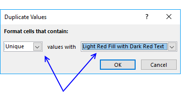
- Press with mouse on the leftmost drop-down list and change it to «Unique»
- Pick a formatting if you like
- Press with left mouse button on OK button
The picture above shows you, for example, that the first name in the list has a duplicate so that name is not highlighted in any cell.
11.2 Sort unique values at the top
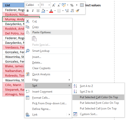
Tip! Did you know that you can put highlighted values to the top
- Press with right mouse button on on a highlighted cell

- Press with mouse on «Sort»
- Press with mouse on «Put Selected Cell Color On Top»
Back to top
12. Useful tips
12.1 Excel tables
An Excel Table is a great feature and is very cleverly designed. It is constructed to automatically expand if you add more data which is incredibly helpful. You don’t need to do anything, not adjusting cell references which is time consuming and prone to errors.
Structured references are cell references to an excel defined table. They let you easily see what the data contains as long as you give it good descriptive column header names.
I recommend you use excel defined tables instead of named ranges or dynamic named ranges as long as you are working with more than one value.
Here is how to convert a list to an excel defined table:
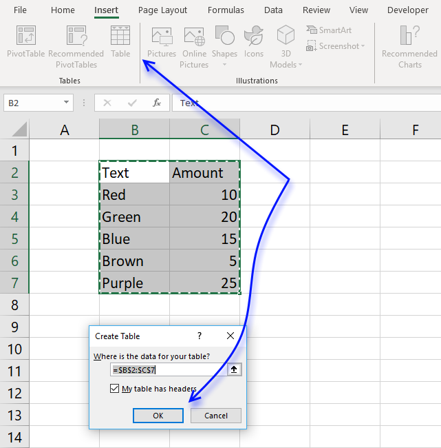
- Select a cell in your list
- Go to tab «Insert» on the ribbon and press with left mouse button on Table button or press Ctrl + T
- Press with left mouse button on OK button
- Your excel defined table is created
Read more about excel defined tables
Back to top
12.2 Named ranges
In excel you can name a cell range, a constant or a formula. You can then use the named range in a formula, making it easier for you to read and understand formulas.
Example
List : A2:A20
Tip! Use dynamic named ranges to automatically adjust cell ranges when new values are added or removed.
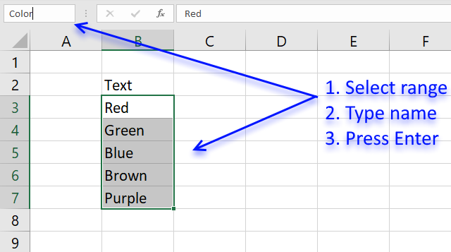
12.2.1 How to create a named range
The downside with named ranges is that you need to adjust the range every time you add or delete a value in the list, the named range will then not fit the value list. I recommend using excel defined tables if you know that the list may change in the future.
- Select cell range B3:B7
- Type Color in name box
- Press Enter
Formula example containing name range:
=INDEX(Color,MATCH(0,COUNTIF($C$2:C2,Color),0))
Back to top
13. How to remove errors (Excel 2007)
Excel 2007 users (and later versions) can remove errors using IFERROR() function.
When the formula runs out of values it returns #N/A errors (Not Available), you can use the IFERROR function to remove the error and return blanks in those cells.
Unfortunately, it comes with a big disadvantage, it also removes other formula errors as well. So use this with great caution. If your source table has errors you won’t detect it because the IFERROR function returns a blank cell instead.
Array formula in cell D2:
=IFERROR(LOOKUP(2, 1/(COUNTIF($D$2:D2, $B$3:$B$21)=0), $B$3:$B$21), «»)
and copy it down as far as necessary.
Back to top
Recommended articles
How to use the IFERROR function
How to use the ISERROR function
How to use the ERROR.TYPE function
How to find errors in a worksheet
Delete blanks and errors in a list
Back to top
14. Excel 2003 users can remove errors using isna() function:
=IF(ISNA(INDEX($A$2:$A$20, MATCH(0, COUNTIF($B$1:B1, $A$2:$A$20), 0))), «», INDEX($A$2:$A$20, MATCH(0, COUNTIF($B$1:B1, $A$2:$A$20), 0)))
and copy it down as far as needed.
This formula is an array formula, how to enter an array formula.
Recommended article
- ISNA function
Back to top
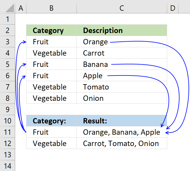
15. How to ignore blank cells in a range
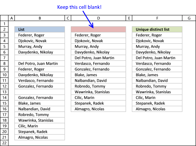
Harlan Grove created a formula to count unique distinct values from a list with blanks. I used the same technique here to filter unique distinct values in column D.
If you want a header name you can use the slightly larger formula, displayed in column F below.
Update 2020-12-09, Excel 365 users can use this regular formula:
=UNIQUE(FILTER($B$3:$B$21, ($B$3:$B$21<>»») * ($B$3:$B$21<>»»)))
The formula below is actually 58 character while the new Excel 365 formula above is 61 characters, space characters not included. You can find a formula explanation here: Extract unique distinct values ignoring blanks
Use the formula below if you have an earlier Excel version than Excel 365.
Update 2017-09-01, smaller regular formula in cell D3:
=LOOKUP(2, 1/(COUNTIF($D$2:D2, $B$3:$B$21&»»)=0), $B$3:$B$21)
Formula in cell F3 if you need a column header name:
=LOOKUP(2, 1/((COUNTIF($F$2:F2, $B$3:$B$21)+($B$3:$B$21=»»))=0), $B$3:$B$21)
15.1 Watch a video where I explain how these two formulas work
Subscribe to Get Digital Help on Youtube:
This article shows you how to fill blank cells with values or formulas
Recommended articles
Learn how to extract non-blank cells in a list using a formula:
Recommended articles
![]()
Remove blank cells
In this blog post I will provide two solutions on how to remove blank cells and a solution on how […]
Back to top
15.2 Get Excel file
Back to top
Very often we need to get distinct or unique value from a column in Excel. In SQL, it is as simple as Select Distinct. However, we don’t have such thing as Select distinct in Excel. What should we do?
No worries at all! There are a couple of ways to get distinct values in Excel.
In this article, I will show you 6 different ways. They are “Remove duplicates”, “Advanced filter”, “Function”, “Formula”, “Pivot table” and “VBA” respectively.
These ways allow you to deal with almost all kinds of situation when it comes to getting unique values in Excel.
You may also be interested in How to Generate Random Dates in Excel
Example
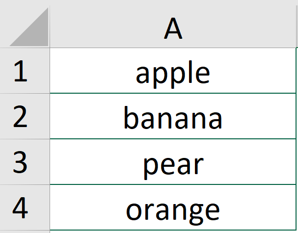
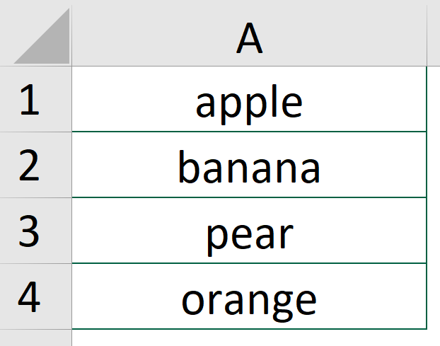
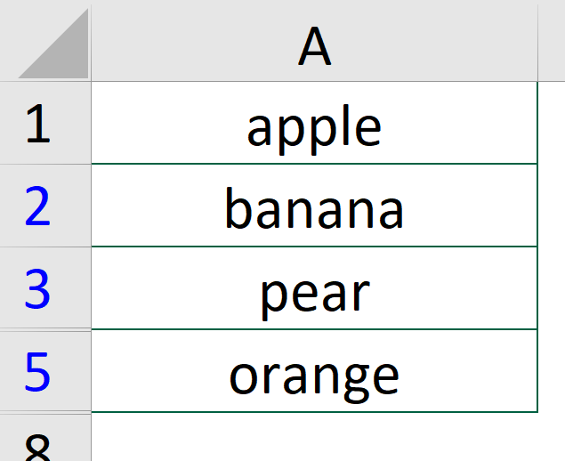
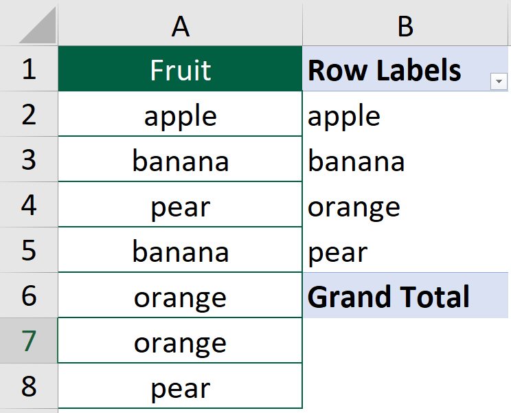
In this article, we will be using the following list as an example.
On the list, there are “apple”, “banana”, “pear”, “banana”, “orange”, “orange” and “pear” respectively.
Among the list of value, there are a few number of duplicates.
If we are to get the distinct value from the list, they would be “apple”, “banana”, “pear” and “orange”.
It is easy to spot the distinct value if the list is short but that is usually not the case. That is why we will need the following solutions.
Get distinct values in Excel by Remove Duplicates
Step 1: Select the data range
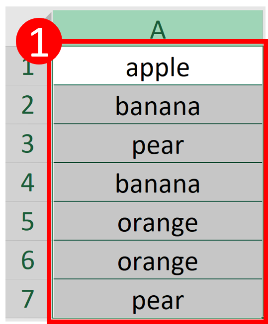
Step 2: Select Remove Duplicates
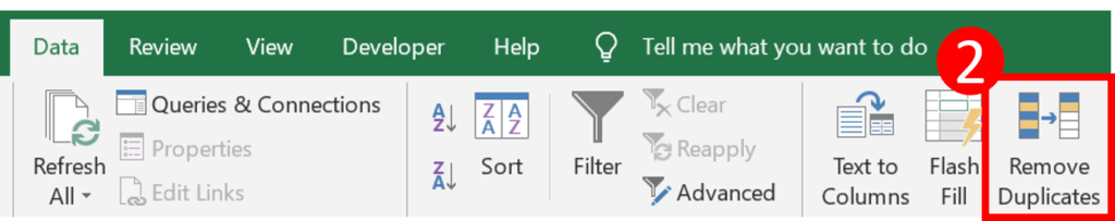
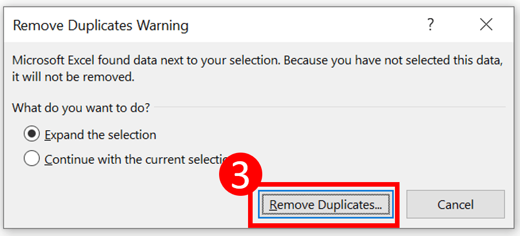
Step 3: Press Remove Duplicates
Result
Get distinct values in Excel by Advanced Filter
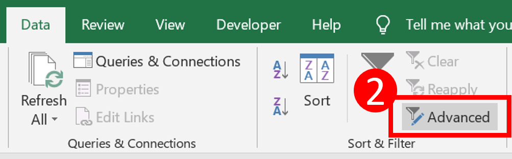
Step 1: Select the data range
Step 2: Select Advanced
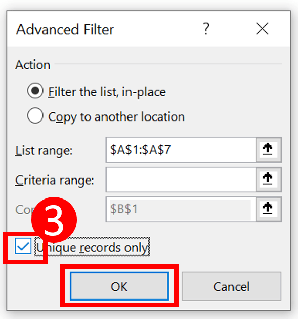
Step 3: Check Unique records only and press OK
Result
You may be interested in How To Center Cells Across Multiple Columns?
Get distinct values in Excel by Function
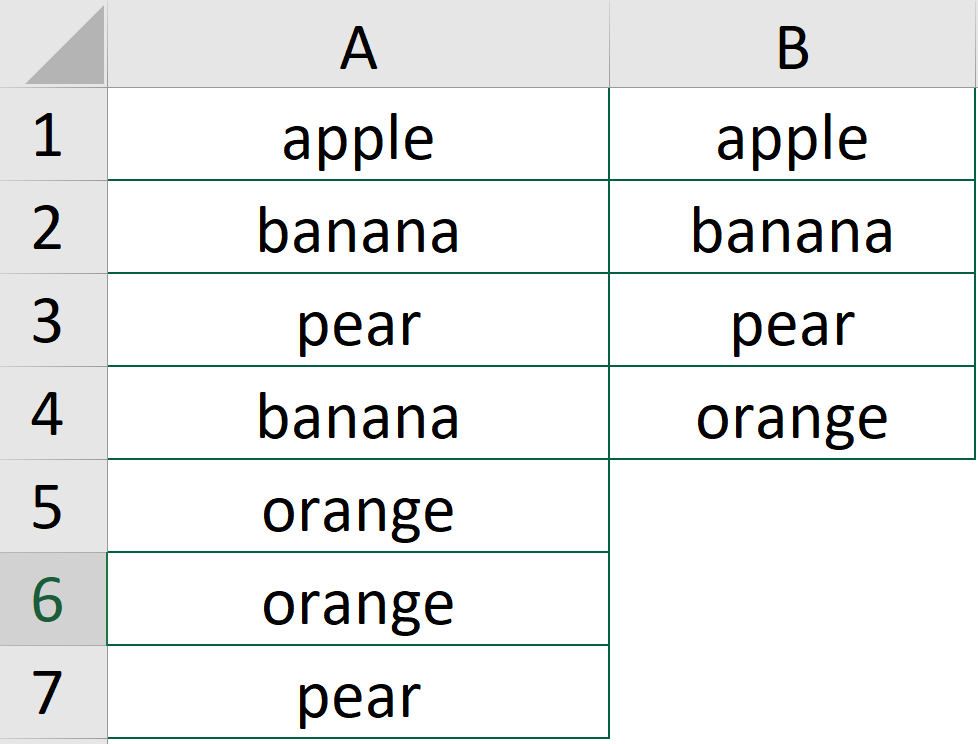
UNIQUE function Syntax
UNIQUE(array, [by_col], [occurs_once])
Formula of Cell B1
=UNIQUE(A1:A7)
Result
You may be interested in How To Reverse Concatenate In Excel (3 ways)?
Get distinct values in Excel by By Formula
UNIQUE function is purposefully made to get a distinct list of values. The only downside is that UNIQUE() is currently available in certain version of Excel. Not every Excel users get to use this wonderful function.
Fortunately, we can use a formula to replicate the UNIQUE function. The formula is a bit long yet not as complicated as many people think.
To get a better understanding of this formula, you may want to check out How to Get Unique Values Without Unique function? The article explains the formula in details.
Standard Formula
=IFERROR(INDEX($A$2:$A$9,MATCH(0,INDEX(COUNTIF($C$1:C1,$A$2:$A$9),0,0),0)),"")
Array Formula
=IFERROR(INDEX($A$2:$A$9, MATCH(0, COUNTIF($C$1:C1, $A$2:$A$9), 0)), "")
Result
You may be interested in How to Sum Intersections of Multiple Ranges?
Get distinct values in Excel by By Pivot table
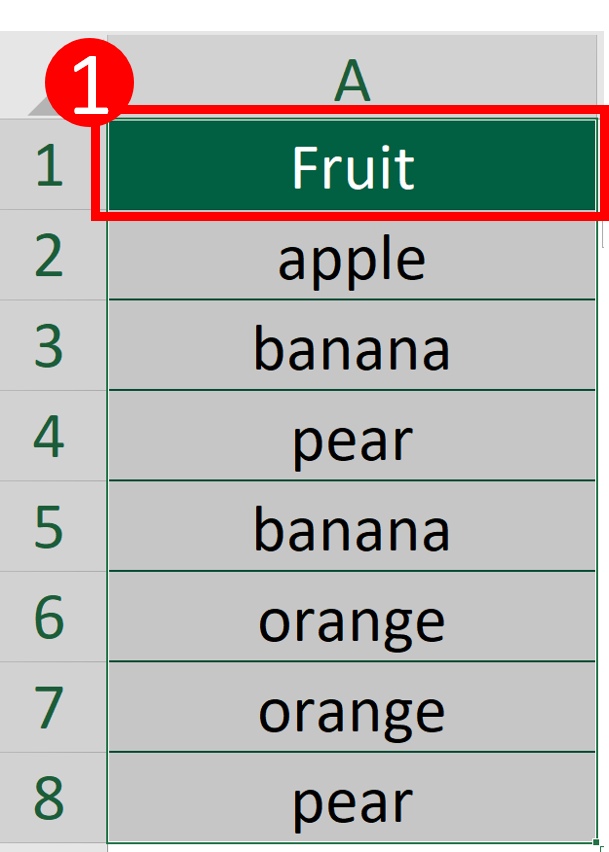
Step 1: Select the data range
Make you give your data range a header or things may go wrong.
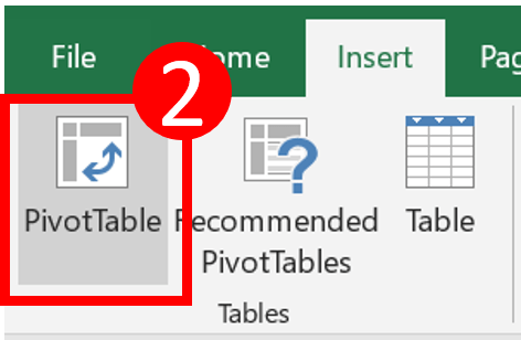
Step 2: Select PivotTable
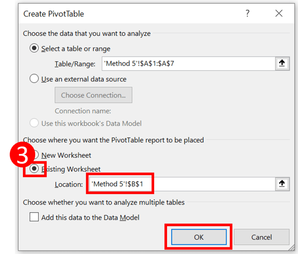
Step 3: Select Existing Worksheet, choose a location and press OK
I selected cell B1 as the location.
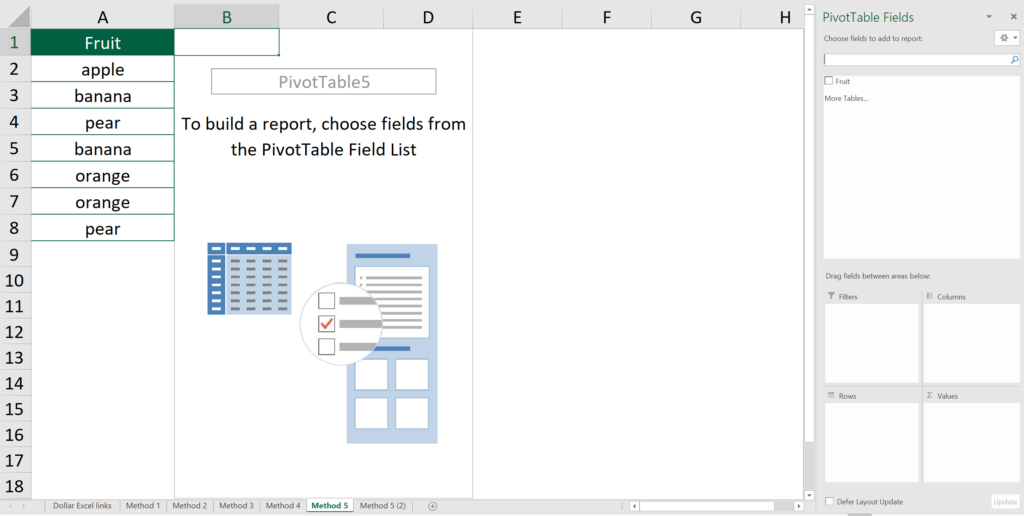
Now your Excel should become like this.
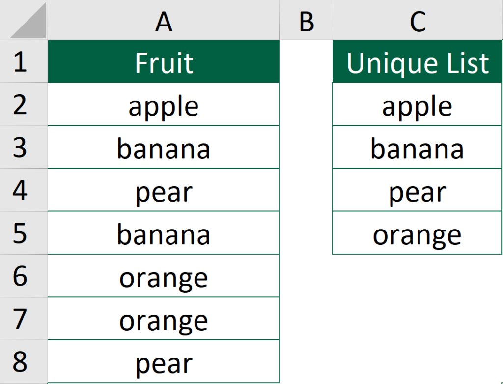
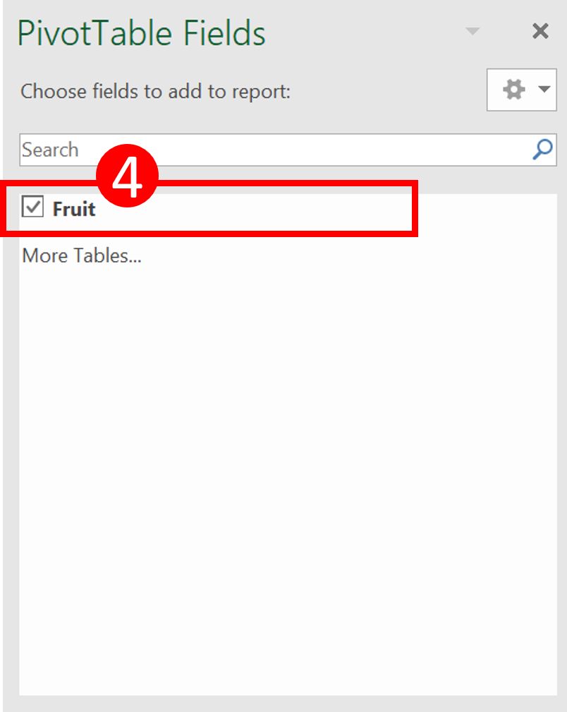
Step 4: Select the field
The top cell in your data range will be perceived by Excel as the name column header.
By selecting “Fruit”, you are basically telling Excel “Please show the column in my PivotTable”.
Result
The PivotTable automatically shows distinct values only.
You may be interested in How to use REPT functions to the Most.
Get distinct values in Excel by VBA
Check out How to Insert & Run VBA code in Excel – VBA101 to see why you should learn VBA.
So basically we are trying to do the following things:
- Identify cells that are not unique
- Delete those cells
Below are the code that does the things we suggested above.
How to use the code
Step 1: Select cell ranges
Step 2: Run the code
Sub GetDistinctvalue()
    'perform the code only when the active cell is not equal to zero
    Do While ActiveCell.Value <> ""
        'If the value of the cell in loop is equal to any of the cell selected
        If ActiveCell.Value = ActiveCell.Offset(1, 0).Value Then
            'Select the active cell
            ActiveCell.Select
            'Delete it and move the remaining cells upward so there should be no blank cell
            Selection.Delete Shift:=xlUp
        Else
            'Make the next cell in selection active
            ActiveCell.Offset(1, 0).Activate
        End If
    Loop
End Sub
Result
You may be interested in How to use REPT functions to the Most.
Hungry for more useful Excel tips like this? Subscribe to our newsletter to make sure you won’t miss out on any of our posts and get exclusive Excel tips!