
![]()
When you create a pivot table to summarize data, Excel automatically creates sums and counts for the fields that you add to the Values area. In addition, you might want to see a distinct count (unique count) for some fields, such as:
- The number of distinct salespeople who made sales in each region
- The count of unique products that were sold in each store
Normal Pivot Tables
For a normal pivot table, there isn’t a built-in distinct count feature in a normal pivot table. However, in Excel 2013 and later versions, you can use a simple trick, described below, to show a distinct count for a field.
For older versions of Excel, try one of the following methods:
- In Excel 2010, use a technique to “Pivot the Pivot table”.
- In Excel 2007 and earlier versions, add a new column to the source data, and Use CountIf.
Add to Data Model – Excel 2013 and Later
In Excel 2013, if you add a pivot table’s source data to the workbook’s Data Model, it is easy to create a distinct count in Excel pivot table.
NOTE: This technique creates an OLAP-based pivot table, which has some limitations, such as no ability to add calculated fields or calculated items. If you need the restricted features, try the “Pivot the Pivot” method instead.

The Sample Data
In this example, there are 4999 records that show product sales, with the region and salesperson name. The first few records are shown in the screen shot below.
You can download the sample workbook from my Contextures website. On the Pivot Table Unique Count page, go to the Download section, and click the link.

Create the Pivot Table
First, to create a pivot table that will show a distinct count, follow these steps:
- Select a cell in the source data table.
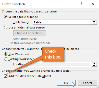
- At the bottom of the Create PivotTable dialog box, add a check mark to “Add this data to the Data Model”
- Click OK

Set up the Pivot Table Layout
To set up the pivot table layout, follow these steps:
- In the pivot table, add Region to the Row area.
- Add these 3 fields to the Values area — Person, Units, Value
- The Person field contains text, so it defaults to Count of Person. The count shows the total number of transactions in each region, not a unique count of salespeople

Show a Distinct Count
To get a unique count (distinct count) of salespeople in each region, follow these steps:
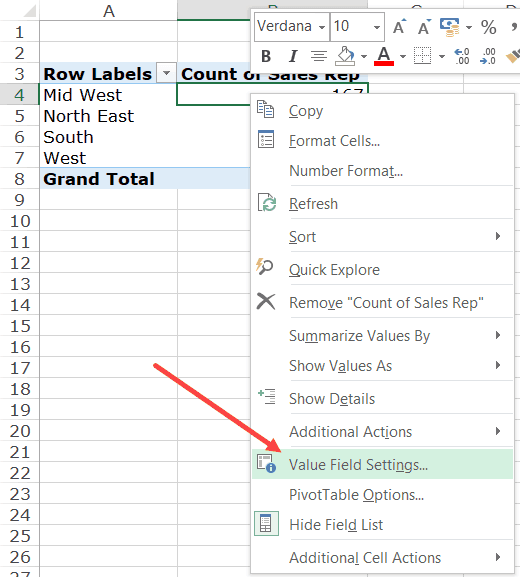
- Right-click one of the values in the Person field
- Click Value Field Settings

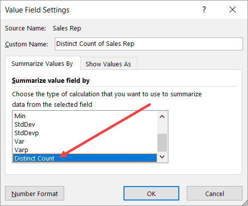
- In the Summarize Value Field By list, scroll to the bottom, and click Distinct Count, then click OK

The Person field changes, and instead of showing the total count of transactions, it shows a distinct count of salespeople names.

Distinct Count in Excel Pivot Table Workbook
To download the sample workbook, go to the Pivot Table Unique Count page, on my Contextures website. On that page, go to the Download section, and click the link.
That page also has instructions for calculating a unique count in older versions of Excel.
_________________________
Excel Pivot Tables are amazing (I know I mention this every time I write about Pivot Tables, but it’s true).
With a basic understanding and a little drag and drop, you can get a bucket-load of work done in a few seconds.
While a lot can be done with a few clicks in Pivot Tables, there are some things that would need a few extra steps or a little bit of work around.
And one such thing is to count distinct values in a Pivot Table.
In this tutorial, I will show you how to count distinct values as well as Unique Values in an Excel Pivot table.
But before I jump into how to count distinct values, it’s important to understand the difference between ‘distinct count’ and ‘unique count’
Distinct Count Vs Unique Count
While these may seem like the same thing, it’s not.
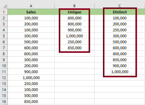
Below is an example where there is a dataset of names and I have listed unique and distinct names separately.
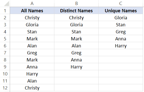
Unique values/names are those that only occur once. This means that all the names that repeat and have duplicates are not unique. Unique names are listed in column C in the above dataset
Distinct values/names are those that occur at least once in the dataset. So if a name appears three times, it’s still counted as one distinct name. This can be achieved by removing the duplicate values/names and keeping all the distinct ones. Distinct names are listed in column B in the above data set.
Based on what I have seen, most of the times when people say that they want to get the unique count in a Pivot Table, they actually mean distinct count, which is what I am covering in this tutorial.
Count Distinct Values in Excel Pivot Table
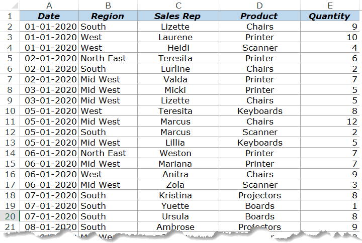
Suppose you have the sales data as shown below:
Click here to download the example file and follow along
With the above dataset, let’s say that you want to find the answer to the following questions:
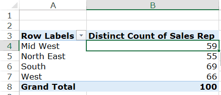
- How many sales rep are there in each region (which is nothing but the distinct count of sales reps in each region)?
- How many sales rep sold the printer in 2020?
While Pivot Tables can instantly summarize the data with a few clicks, to get the count of distinct values, you will need to take a few more steps.
If you’re using Excel 2013 or versions after that, there is an inbuilt functionality in Pivot Table that quickly gives you the distinct count. And if you’re using Excel 2010 or versions before that, you will have to modify the source data by adding a helper column.
The following two methods are covered in this tutorial:
- Adding a helper column in the original data set to count unique values (works in all versions).
- Adding the data to a data model and using Distinct Count option (available in Excel 2013 and versions after that).
There is a third method which Roger shows in this article (which he calls the Pivot the Pivot Table method).
Let’s get started!
Adding a Helper Column in the Dataset
Note: If you’re using Excel 2013 and higher versions, skip this method and move to the next one (as it uses an inbuilt Pivot Table functionality – Distinct Count).
This is an easy way to count distinct values in the Pivot Table as you only need to add a helper column to the source data. Once you have added a helper column, you can then use this new data set to calculate the distinct count.
While this is an easy workaround, there are some drawbacks to this method (covered later in this tutorial).
Let me first show you how to add a helper column and get a distinct count.
Suppose I have the data set as shown below:
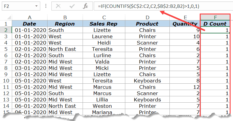
Add the following formula in Column F and apply it for all the cells that have data in the adjacent columns.
=IF(COUNTIFS($C$2:C2,C2,$B$2:B2,B2)>1,0,1)
The above formula uses the COUNTIFS function to count the number of times a name appears in the given region. Also, note that the criteria range is $C$2:C2 and $B$2:B2. This means that it keeps expanding as you go down the column.
For example, in cell E2, the criteria ranges are $C$2:C2 and $B$2:B2 and in cell E3 these ranges expand to $C$2:C3 and $B$2:B3.
This ensures that the COUNTIFS function counts the first instance of a name as 1, the second instance of the name as 2, and so on.
Since we only want to get the distinct names, the IF function is used which returns 1 when a name appears for a region the first time and returns 0 when it appears again. This makes sure that only distinct names are counted and not the repeats.
Below is how your dataset would look like when you have added the helper column.
Now that we have modified the source data, we can use this to create a Pivot Table and use the helper column to get the distinct count of the sales rep in each region.
Below are the steps to do this:
- Select any cell in the dataset.
- Click the Insert Tab.

- Click on Pivot Table (or use the keyboard shortcut – ALT + N + V)
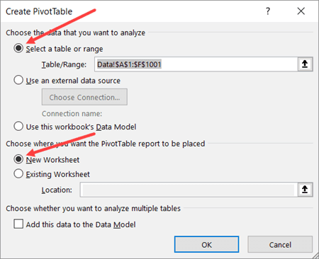
- In the Create Pivot Table dialog box, make sure that the Table/Range is correct (and includes the helper column) and’New Worksheet’ in selected.

- Click OK.


The above steps would insert a new sheet which has the Pivot Table.
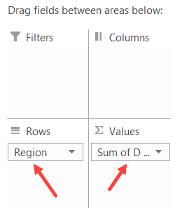
Drag the ‘Region’ field in the Rows area and ‘D Count’ field in the Values area.
You will get a Pivot Table as shown below:
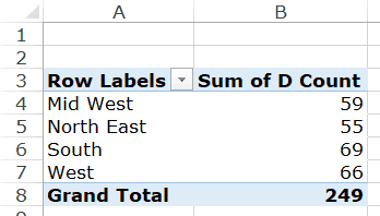
Now you can change the column header from ‘Sum of D count’ to ‘Sales Rep’.
Drawbacks of Using a Helper Column:
While this method is pretty straight forward, I must highlight a few drawbacks that come with modifying the source data in a Pivot Table:
- The data source with the helper column is not as dynamic as a Pivot Table. While you can slice and dice the data any way you want with a Pivot Table, when you use a helper column, you lose a part of that ability. Let’s say that you add a helper column to get the count of a distinct sales rep in each region. Now, what if you also want to get the distinct count of sales rep selling printers. You will have to go back to the source data and modify the helper column formula (or add a new helper column).
- Since you’re adding more data to the Pivot Table source (which also gets added to the Pivot Cache), this can lead to a higher size of Excel file.
- Since we are using an Excel formula, it may make your Excel Workbook slow in case you have thousands of rows of data.
Add Data to Data Model and Summarize Using Distinct Count
Pivot Table added new functionality in Excel 2013 that allows you to get the distinct count while summarizing the data set.
In case you’re using a previous version, you’ll not be able to use this method (as should try adding the helper column as shown in the method above this one).
Suppose you have a dataset as shown below and you want to get the count of the unique sales rep in each region.
Below are the steps to get a distinct count value in the Pivot Table:
- Select any cell in the dataset.
- Click the Insert Tab.
- Click on Pivot Table (or use the keyboard shortcut – ALT + N + V)
- In the Create Pivot Table dialog box, make sure that the Table/Range is correct and New Worksheet in Selected.
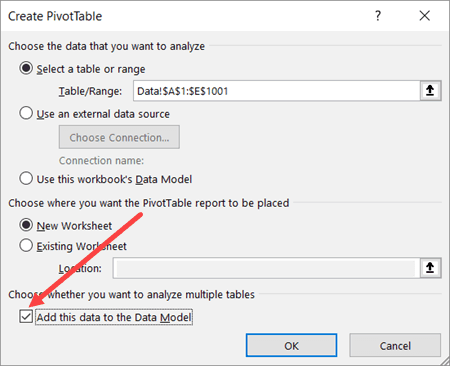
- Check the box which says – “Add this data to the Data Model”
- Click OK.
The above steps would insert a new sheet which has the new Pivot Table.
Drag the Region in the Rows area and Sales Rep in the Values area. You will get a Pivot Table as shown below:
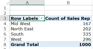
The above Pivot Table gives the total count of the Sales rep in each region (and not the distinct count).
To get the distinct count in the Pivot Table, follow the below steps:
- Right-click on any cell in the ‘Count of Sales Rep’ column.
- Click on Value Field Settings

- In the Value Field Settings dialog box, select ‘Distinct Count’ as the type of calculation (you may have to scroll down the list to find it).

- Click OK.
You will notice that the name of the column changes from ‘Count of Sales Rep’ to ‘Distinct Count of Sales Rep’. You can change it to whatever you want.
Some things you know when you add your data to the Data Model:
- If you save your data in the data model and then open in an older version of Excel, it will show you a warning – ‘Some pivot table functions will not be saved’. You may not see the distinct count (and the data model) when opened in an older version that doesn’t support it.
- When you add your data to a Data Model and make a Pivot Table, it will not show the options to add calculated fields and calculated columns.
Click here to download the example file
What If You Want to Count Unique Values (and not distinct values)?
If you want to count unique values, you don’t have any inbuilt functionality in the Pivot Table and will have to rely on helper columns only.
Remember – Unique values and distinct values are not the same. Click here to know the difference.
One example could be when you have the below data set and you want to find out how many sales rep are unique to each region. This means that they operate in one specific region only and not the others.
In such cases, you need to create one of more than one helper columns.
For this case, the below formula does the trick:
=IF(IF(COUNTIFS($C$2:$C$1001,C2,$B$2:$B$1001,B2)/COUNTIF($C$2:$C$1001,C2)<1,0,1),IF(COUNTIF($C2:C$22,C2)>1,0,1),0)
The above formula checks whether a sales rep name occurs in one region only or in more than one region. It does that by counting the number of occurrence of a name in a region and dividing it by the total number of occurrences of the name. If the value is less than 1, it indicates that the name occurs in two or more than two regions.
In case the name occurs in more than one region, it returns a 0 else it returns a one.
The formula also checks whether the name is repeated in the same region or not. If the name is repeated, only the first instance of the name returns the value 1, and all other instances return 0.
This may seem a bit complex, but it again depends on what you’re trying to achieve.
So, if you want to count unique values in a Pivot Table, use helper columns and if you want to count distinct values, you can use the inbuilt functionality (in Excel 2013 and above) or can use a helper column.
Click here to download the example file
You May Also Like the Following Pivot Table Tutorials:
- How to Filter Data in a Pivot Table in Excel
- How to Group Dates in Pivot Tables in Excel
- How to Group Numbers in Pivot Table in Excel
- How to Apply Conditional Formatting in a Pivot Table in Excel
- Slicers in Excel Pivot Table
- How to Refresh Pivot Table in Excel
- Delete a Pivot Table in Excel
Bottom Line: Learn two ways to solve the data analysis challenge, calculating distinct count, with pivot tables.
Skill Level: Intermediate
Video Tutorial
Download the Excel File
I’ve included both the original file and the solution file for you to download here:
Counting Unique Rows
In this post, we’re going to take a look at two different ways to do a distinct count using pivot tables. These two methods were submitted as solutions to the data analysis challenge that you can find here:
Excel Data Analysis Challenge
To summarize the challenge, we want to create a summary report of deal count by stage, but there are multiple rows per deal in the CRM data. So we have to find a way to create a distinct count (counting unique rows) for each deal so that we can sum them up.
By the way, thank you to anyone who submitted a solution to the data challenge! There were a lot of great submissions.
Solution #1 – Using a Helper Column
The great thing about this solution is that it can be used in any version of Excel.
Start by turning your data into an Excel Table. To do that, just select any cell in the data set, and click on Format as Table on the Home tab. Right-click on the table format you want and select Apply and Clear Formatting.
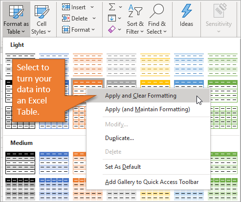
Hit OK when the Format as Table window appears.
Now that your data is in Table format, add a helper column to the right of the table and label it Deal Count. Use the COUNTIF function, with the range being the Deal ID column, and the criteria being the cell in the Deal ID column that corresponds with the row you are in.
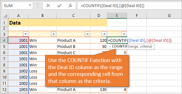
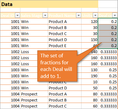
The formula will return the number of rows for each Deal ID number. If we divide the formula into the number 1, we will get fractions in each of those cells that when added together will count one entry for each deal.
The change to the formula can be seen in green here:
=1/COUNTIF([Deal ID],[@[Deal ID]])
Now that we have these fractions that will give us a distinct count when we create our pivot table, we can go ahead and create the pivot table by choosing Pivot Table on the Insert tab.
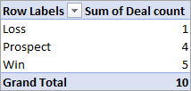
To create our summary report using the new pivot table, put the Sales Stage in the Rows area and Deal Count in the Sum of Values area.
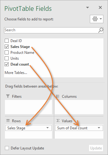
This will give us the summary report we are looking for, with a count of deals in each sale stage.
The nice thing about using a pivot table is that as we add or delete source data entries, we can refresh the pivot table ( Alt + F5 ) to include those changes.
Solution # 2 – Using Power Pivot
This solution is only available for versions of Excel that are 2013 or later for Windows.
We still want our data formatted as an Excel Table, but we don’t need a helper column for this solution.
This time, when we create our pivot table, we are going to check the box that says Add this table to the Data Model. (Data Model is another term for PowerPivot.)
When you build your pivot table this time, you are going to drag Deal ID to the Sum of Values area.
That initially gives us numbers we don’t want in our summary report. To fix this, we want to right-click on the Sum of Deal ID column header and select Value Field Settings. This will open a window where we can choose Distinct Count as a calculation type.
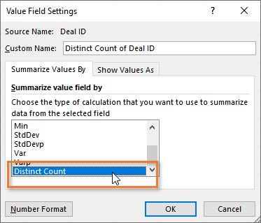
The Distinct Count function goes through the Deal ID column and gives us a count of the unique values, so our summary report will look just like it did for Solution #1.
Comparing the Two Solutions
Both of these solutions are great because they can be refreshed when new data is added to the source table.
The advantage to Solution #1 is that it can be done in any version of Excel. With that said, if you are running 2013 or later in Windows, Solution #2 is the superior option. This is because Solution #1 gets wonky when you try to filter the data down (say, for a certain product) or use slicers to dissect the data further.
If you’d like to learn more about using Pivot Tables, I have a separate blog post you can check out here: Introduction to Pivot Tables and Dashboards.
Other Solutions
There were lots of other great solutions to the challenge that were submitted. They included using Power Query and new dynamic functions. We will take a look at those in future posts, but I wanted to start with these two because they were more universal in terms of Excel version access.
If you have questions about either of these solutions, please leave a comment below!
In this article, we’ll talk through how to get distinct count in Excel pivot table. MS Excel has a powerful tool that can display a standard count and a distinct count.
In addition to that, you’ll learn the difference between unique values and distinct values. We’ll also show you how to get unique values in Excel using formulas.
Start to learn, understand, and know how to use and get distinct counts in Excel pivot tables and using formulas with this comprehensive guide that will ease your work.
A distinct count in Excel pivot tables is one of the powerful tools in Excel that allows you to count and determine the number of unique values in a given data set. In addition to that, it has always been equal to or less than count.
Count is different from distinct because count is the total number of values, and it counts the duplicate values. However, distinct count is the total of different values or the number of unique values, and it doesn’t include duplicate values.
What is the Difference between Unique Count and Distinct Count?
| Unique values | Distinct values |
|---|---|
| Unique count is the total number of values that occur only once in the data set. | Distinct count is the total number of different values nevertheless it occurs many times still it is counted as one distinct count. |
In a very brief statement, values that are repeats or duplicates are not unique. Whereas distinct are those values that appear at once, even if the value appears multiple times, it is still counted as one.
Let’s take a look at our example below:
As you can see in the image, you can easily determine the difference between the two data sets.
Note: Unique and distinct count are not thesame.
How to use and get distinct counts in an Excel pivot table
This time, we will explore how to get unique and distinct values in Excel using formulas, and we’ll also show you how to use distinct counts in an Excel pivot table.
Adding a Distinct Count in Excel using Pivot Table
Using a data model is the best and easiest way to get a distinct count in Excel. Follow the following guide:
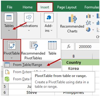
- Click the cell that contains your data, and then click “Insert” in the menu bar.
- Click “Tables,” and it will show the list of tables.
- Select “From Pivot Table/Range.” It will show a dialog box.
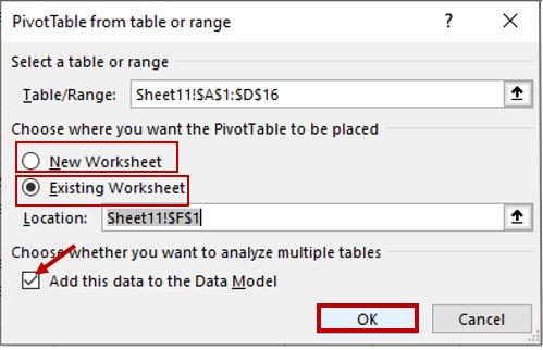
- In “PivotTable from or range,” dialog box you can choose where you want to put your pivot table, either in a new worksheet or an existing worksheet. In our case, we chose “Existing Worksheet.”
- When you choose “Existing Worksheet,” you have to click any cell where you want to display your pivot table in your current worksheet, and then it will display in the “Location.”
- But if you choose “New Worksheet,” it will open a new worksheet.
- Don’t forget to check the checkbox “Add this data to the Data Model.”
- Then click “OK.”
9. It will look like this after you click “OK.”
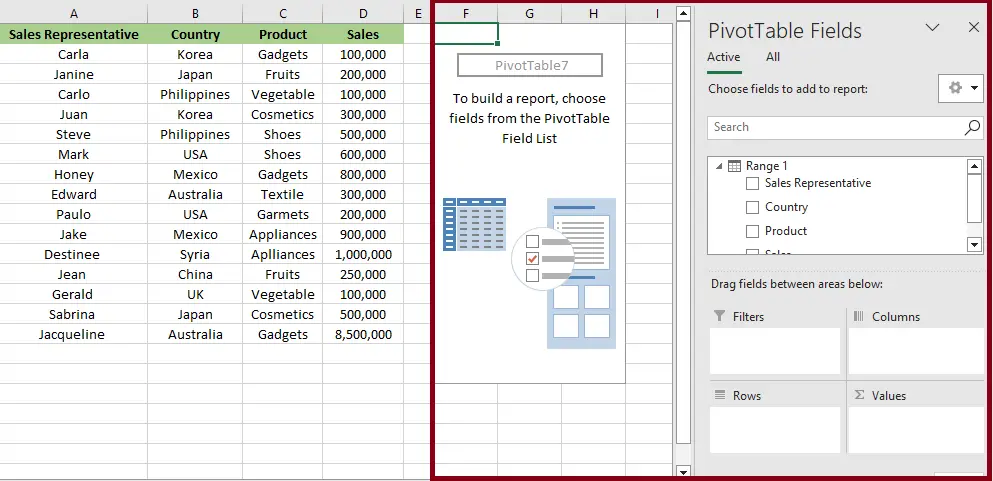
10. Now it’s time to get a distinct count, but first we have to add data to your pivot table layout.
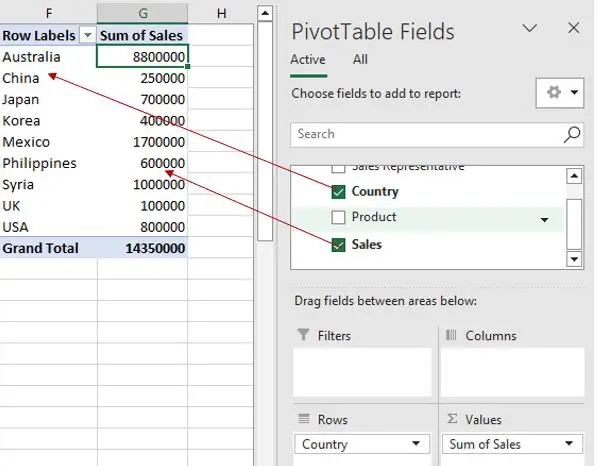
11. Right-click the value of “Sum of Sales” in our case, then click “Summarize Values By” and choose “Distinct Count.”
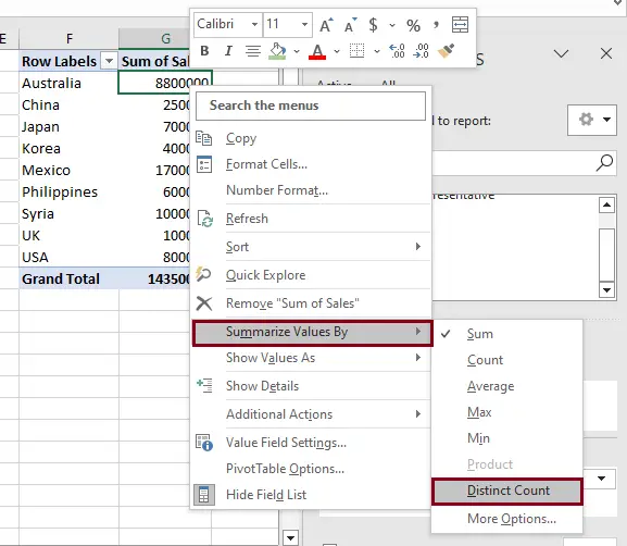
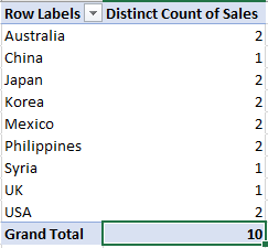
12. As a result, you’ll get a 10 distinct count for sales in the pivot table.
Kindly check the video below; it contains a step-by-step guide from the beginning and different ways on how to get a distinct count in Excel pivot table.
Note: For those who are using Excel 2013, 2016, 2019, and Microsoft 365, the only thing you do is access the data model.
Adding a Distinct Count in Excel using the Function
To get the distinct count without using a pivot table in Excel, you just need the formula in order to get the distinct values. Especially when you are holding huge amounts of data, we know that it’s hard to do it manually.
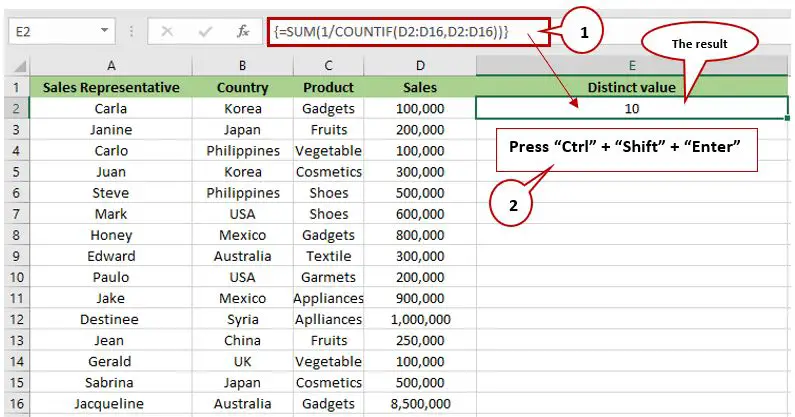
We need to use this formula: = SUM(1/COUNTIF(range, range)). Why do we use COUNTIF? It is because we need to find out how many times each value appears on your worksheet, particularly within the specific range.
Take a look at our example below:
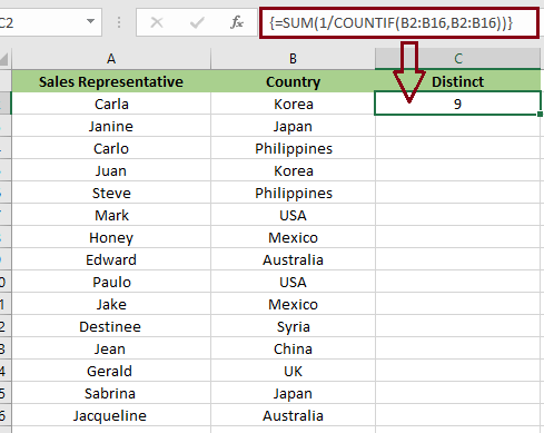
Note: Don't put a bracket sign in your formula bar; it only appears due to the shortcut key that we use, "Ctrl" + "Shift" + "Enter," in order to get the exact value.
Formula to get a distinct count in Excel
1. =SUM(IF(1/COUNTIF(data, data)=1,1,0))
Note: You have to press the "Ctrl" + "Shift" + "Enter" shortcut rather than the usual Enter keystroke, because it is an array formula.
2. =SUMPRODUCT(1/COUNTIF(range, range))
Tip: if you want the usual keystrokes, you may use the formula above.
Counting Distinct numbers using a Formula
Use ISNUMBER to get the distinct count values (time, date, and number) in Excel.
Here’s the formula: =SUM(IF(ISNUMBER(range) or = 1/COUNTIF(range, range),””)).
Here’s the thing that you should do:
- Click the cell where you want to put the data. Then, input the formula in the formula bar.
- Right after you create the formula, don’t press Enter right away.
- Press “Ctrl” + “Shift” + “Enter” to get the exact value.
Counting Unique and Distinct Counts in Excel
In our example below, we want to get the unique value of a country using a formula, and we get a value of 3 and a distinct value of 9.
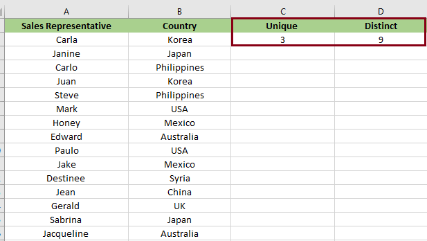
The formula to get the Unique value is =SUM(IF(COUNTIFS(B2:B16,B2:B16)=1,1,0)). Whereas the the formula we use in the example is =SUM(1/COUNTIF(B2:B16,B2:B16)).
Conclusion
This simple tutorial on how to get the distinct count in an Excel pivot table will be able to help you get the value of distinct in a large amount of data. We also provided a formula to get the unique and distinct values in all version of Excel if you don’t want to use a pivot table.
With the help of this guide, you will be able to differentiate between unique and distinct values.
Thank you very much for continuing to read until the end of this article. In case you have more questions, feel free to comment. You can also visit our website for additional information.
Do you need to know how many customers you have invoiced this month? When creating a Pivot Table and adding your customers to both the row labels and again in the value area, each transaction is totaled for each customer. This does not give a true reflection of how many customers you have invoiced.

In Microsoft® Excel® 2013 and 2016, a new feature called “Distinct Count” was added which will return an accurate count of unique customers.
Applies To: Microsoft® Excel® 2013 and 2016.
1. Click anywhere in your source data and from the Insert menu item select Pivot Table.
2. The next step, which is vital, is to select “Add this data to the Data Model”.

3. The Pivot Table is now created and ready for use. Drag and drop “CustomerName” in the Row and Values areas.

4. Your Pivot Table will now display, as can be seen below, which is not a true reflection of how many customers have been invoiced, but a count of how many transactions took place.

5. To get a unique count of customers, click on the “count of CustomerNames” drop down and select “Value Field Settings”

6. Under the “Summarize Value Field By” section, scroll down to the bottom and select “Distinct Count” and then OK.

7. When following the above steps an accurate count of the number of customers invoiced will be displayed.
Instead of applying complex formulas, you can use the Distinct Count option to have an accurate count of transactions. This will save time and lead to better decision making as the correct information will be used.