
Home > Microsoft Excel > How to Count Unique Values in Excel? 3 Easy Ways to Count Unique and Distinct Values
(Note: This guide on how to freeze rows in Excel is suitable for all Excel versions including Office 365)
Working with large amounts of data in Excel can be quite difficult. Some values may be repeated more than once. You might have to take into account multiple entries of data while performing any function to upgrade your accuracy. You will also need to count the values to organize or even acquire statistics from the data.
With large data, it would be nearly impossible to count the values manually. Especially, keeping a track of unique or distinct values can be quite arduous. Fortunately in Excel, there are many ways to count unique and distinct values.
You’ll Learn:
- Unique and Distinct Values
- How to Count Unique Values in Excel
- Using SUM, IF, and COUNTIF Functions
- Count Unique Text Values in Excel
- Count Unique Numeric Values in Excel
- Using SUM, IF, and COUNTIF Functions
- How to Count Distinct Values in Excel
- Using Filter Option
- Using SUM and COUNTIF functions
First, let us understand the difference between Unique and Distinct Values.
Unique and Distinct Values
Data can be repeated or unrepeated. These unrepeated data are of two types. They are called unique data and distinct data.
Unique data are those which occur in the dataset only once.
Whereas, distinct data include the duplicate values but count them only once.
I will explain unique and distinct data with an example for better understanding.
Consider an example, where column A has the list of people and column B lists their favorite colors.

In this, red, green, and purple colors occur only once, so they are called unique elements. Therefore the unique elements count is 3
Whereas, there are 8 distinct elements. That is the colors, though repeated are counted once. The colors are red, green, yellow, blue, white, black, gray, and purple. So, the distinct value count is 8.

In this guide, I will show you how to count unique and distinct values in Excel.
Let’s dive in.
How to Count Unique Values in Excel
First, let us see how to count unique values in excel.
Using SUM, IF, and COUNTIF Functions
In Excel, functions are always available to solve any operations. In this case, you can use a combination of SUM, IF and COUNTIF functions to count unique values in Excel.
To count unique values, enter the formula =SUM(IF(COUNTIF(range, range)=1,1,0)) in the desired cell. The range denotes the starting cell and the ending cell.
This is an array formula where the count values are stored in a new array. Since this is an array formula, make sure you press Ctrl+Shift+Enter after entering the formula. Also, note that when you enter the formula, curly braces will automatically populate at the end of them. But, do not enter them manually.
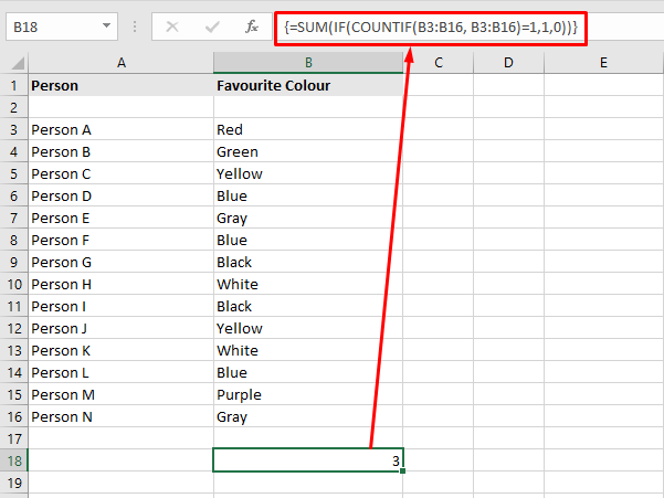
Consider the above example. To calculate the unique values in the given Excel sheet, enter the formula in the destination cell.
In the place of range, enter the cells which contain the elements whose unique value is to be found. Here, cells B3 to B16 house the said elements. So the formula becomes:
=SUM(IF(COUNTIF(B3:B16, B3:B16)=1,1,0))
Now, press Ctrl+Shift +Enter. This gives the count of unique values in the selected range. The unique value count is 3.
Simple, right? Now, let me explain how this formula gives the unique values in 3 simple steps.
- The COUNTIF function counts the number of unique values in the given range B3 to B16. That is the number of times the value is repeated in the range. These counted values are stored in an array. So, the array becomes [1,1,2,3,2,3,2,2,2,2,2,3,1,2]
- Then the IF function keeps the unique values(=1) and replaces anything other than 1 with 0. So the array becomes [1,1,0,0,0,0,0,0,0,0,0,0,1,0]
- Now finally, the SUM function adds the unique value and returns the value 3.
There are two additional cases while using the SUM, IF, and COUNTIF functions. You can use them to find either unique text values or numeric values in Excel.
Count Unique Text Values in Excel
In some tables and worksheets, some texts might be intertwined with numbers. In such cases, you can use the above-mentioned function with a little modification to find the unique text values in Excel.
Enter the formula =SUM(IF(ISTEXT(range)*COUNTIF(range,range)=1,1,0)) in the destination cell and press Ctrl+Shift+Enter. The range denotes the start and end cells that house the elements.
From the general formula, we have added the ISTEXT element to find the unique text values. If the value is a text, the ISTEXT function returns 1 and the value is counted in an array. If the cell houses a non-text value, it returns zero.
The functionality is also similar to the above common formula.
Count Unique Numeric values in Excel
This is a vice versa to the above-mentioned case. In case you only want to count unique numeric values intertwined with texts, you can use the below formula.
Enter the formula =SUM(IF(ISNUMBER(range)*COUNTIF(range,range)=1,1,0)) in the desired cell. The range denotes the start and end cells that hold the values.
Here, the ISNUMBER function returns 1 for numeric values and ignores other values. This function’s working is also similar to the above-mentioned case.
Note: In Excel, date and time are counted as numbers, so they are also counted.
We have seen how to count unique values in excel, we can also count distinct values by using the methods below.
How to Count Distinct Values in Excel
In Excel, there are two easy methods to find the number of distinct values.
Using Filter Option
This is an easy and simple method in Excel which gives you the unique values in your data. In this method, you can use the Filter option to pick out the distinct values. This option filters the elements to another row. then, you can use the ROWS function to find out the number of unique elements.
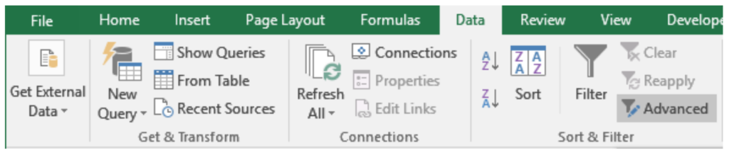
To find the unique rows using the Filter option, first select the rows/columns which have the duplicate elements.
Then, go to Data > Sort & Filter and click on Advanced.
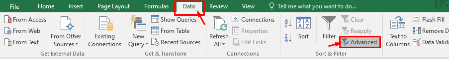
The Advanced Filter dialog box appears.
Specify the List range: i.e select the cells you need to apply the filter to. You can enter them manually, or click on the Collapse button ![]() , select the area and click Expand .
, select the area and click Expand .
First, select the Copy to another location. This copied the unique elements onto a new column.
Now, use the collapse and expand button to select the rows you want the unique elements to be copied.
Finally, check Unique records only. And click OK.
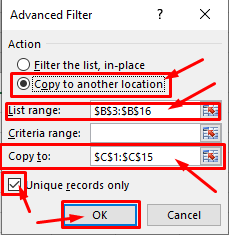
Thus the distinct elements are copied onto a new row.
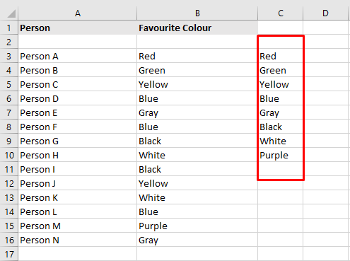
To calculate the row count, you can select the columns and click on Quick analysis or Ctrl + Q. Select Totals and click on Row Count. This will give you the row count right below the unique elements.
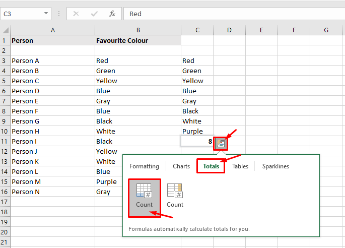
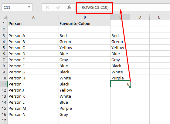
Or, you can use the function =ROWS(a:b), where a and b are the starting and ending cells respectively.
Note: If you click on Filter the list, in-place, the selected values will be replaced in the same column.
Using SUM and COUNTIF functions
You can use the SUM and COUNTIF functions to calculate the distinct values in Excel. In this case, we will inverse the COUNTIF function to arrive at distinct values.
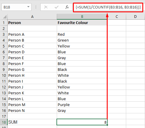
To count distinct values in excel, first enter the formula =SUM(1/COUNTIF(range, range)) in the desired cell. The range specifies the starting cell and ending cell separated by a colon. This is an array function, so press Ctrl+Shift+Enter to apply the formula.

Alternatively, you can also use the formula =SUMPRODUCT(1/COUNTIF(range, range)) in the desired cell to count distinct values. This is not an array function, so pressing Enter is sufficient to apply the formula.
Consider the same above-mentioned example. To count the distinct values, enter the formula =SUM(1/COUNTIF(B3:B16, B3:B16)) in the destination cell. Here, the range is B3:B16, so the values in cells B3 to B16 are taken into account.
First, the COUNTIF function counts the number of times the values occur in the given range. This value is stored in an array. Then, this value is divided by 1. So, if a value occurs twice, the value after dividing by 1 will be 0.5. Now, the SUM or SUMPRODUCT function adds up the fractional values and returns the result which is equal to the count of distinct values in the range.
Note: Similarly, you can also tweak the formulae a little to find distinct text values or distinct numeric values.
To find distinct text values: =SUM(IF(ISTEXT(range),1/COUNTIF(range, range),””))
To find distinct text values: =SUM(IF(ISNUMBER(range),1/COUNTIF(range, range),””))
Closing Thoughts
Finding the unique and distinct elements in a large dataset can be used to determine the statistics or probability of the data.
In this guide, we saw how to count unique and distinct values in Excel. Based on your specifications and preferences, you can either find the count of unique or distinct values.
If you need more high-quality Excel guides, please check out our free Excel resources center.
Simon Sez IT has been teaching Excel for over ten years. For a low, monthly fee you can get access to 100+ IT training courses. Click here for advanced Excel courses with in-depth training modules.
Simon Calder

Chris “Simon” Calder was working as a Project Manager in IT for one of Los Angeles’ most prestigious cultural institutions, LACMA.He taught himself to use Microsoft Project from a giant textbook and hated every moment of it. Online learning was in its infancy then, but he spotted an opportunity and made an online MS Project course — the rest, as they say, is history!
Working with large data sets, we often require the count of unique and distinct values in Excel. Though this may be required in many cases, Excel does not have any pre-defined formula to count unique and distinct values. In this tutorial, you will see a few techniques to count unique and distinct values in Excel.
How to Count Unique and Distinct Values in Excel
The unique values are the ones that appear only once in the list, without any duplications. The distinct values are all the different values in the list.

In this example, you have a list of numbers ranging from 1-6. The unique values are the ones that appear only once in the list, without any duplications. The distinct values are all the different values in the list. The tables below show the unique and distinct values in this list.

Count unique values in Excel
You can use the combination of the SUM and COUNTIF functions to count unique values in Excel. The syntax for this combined formula is = SUM(IF(1/COUNTIF(data, data)=1,1,0)). Here the COUNTIF formula counts the number of times each value in the range appears.
The resulting array looks like {1;2;1;1;1;1}. In the next step, you divide 1 by the resulting values. The IF function implements the logic such that if the values appear only once in the range, this step will generate 1, otherwise it will be a fraction value. The SUM function then sums all the values and returns the result. This is an array formula, so you have to assign it using Ctrl + Shift + Enter.
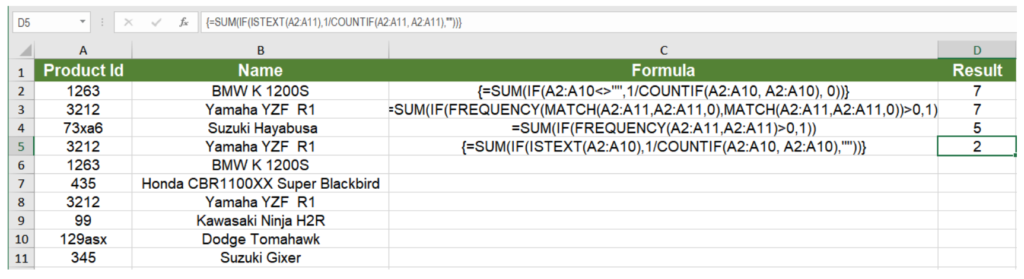
The following example contains a list of automobile products with their product ID and Names. You will count the unique items in this example.
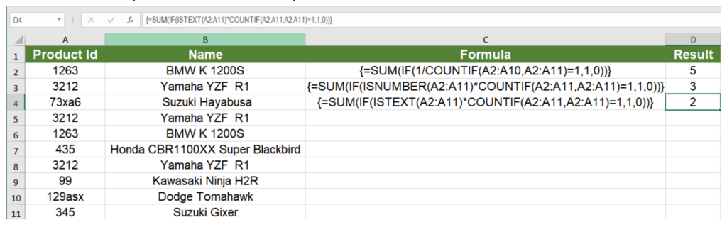
{=SUM(IF(1/COUNTIF(A2:A11,A2:A11)=1,1,0))}
This counts the number of unique values in the list. It follows the syntax mentioned above and returns the count for unique items, which is 5.
{=SUM(IF(ISNUMBER(A2:A11)*COUNTIF(A2:A11,A2:A11)=1,1,0))}
This counts the number of unique numeric values in the list. The only difference with the previous formula is here is the nested ISNUMBER formula that makes sure that you only count the numeric values. Returns the number 3, which is the count of the unique numeric values.
{=SUM(IF(ISTEXT(A2:A10)*COUNTIF(A2:A11,A2:A11)=1,1,0))}
Works the same as the previous formula, counts the unique number of text values instead. The ISTEXT function is used to make sure that only the text values are counted. Returns the number 2.
Count Distinct Values in Excel
Count Distinct Values using a Filter
You can extract the distinct values from a list using the Advanced Filter dialog box and use the ROWS function to count the unique values. To count the distinct values from the previous example:
- Select the range of cells A1:A11.
- Go to Data > Sort & Filter > Advanced.
- In the Advanced Filter dialog box, click Copy to another location.
- Set both List Range and Criteria Range to $A$1:$A$11.
- Set Copy to to $F$2.
- Keep the Unique Records Only box checked. Click OK.
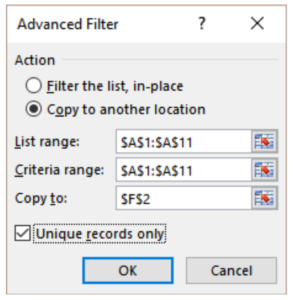
- Column F will now contain the distinct values.
- Select H6.
- Enter the formula
=ROWS(F3:F9). Click Enter.
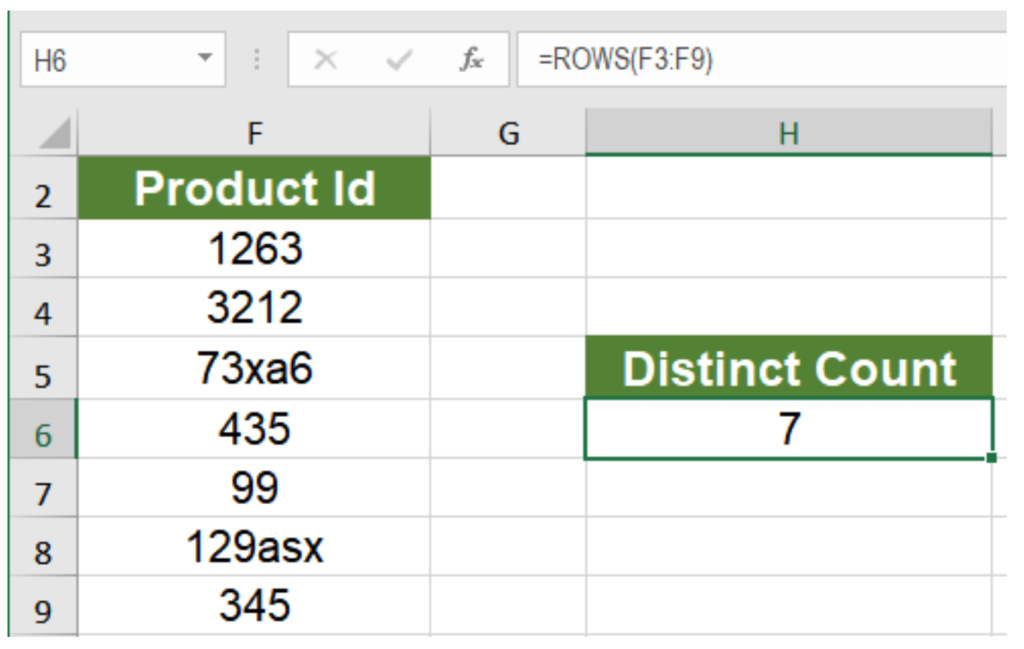
This will show the count of distinct values, 7.
Count Distinct Values using Formulas
You can use the combination of the IF, MATCH, LEN and FREQUENCY functions with the SUM function to count distinct values.
{=SUM(IF(A2:A11<>"",1/COUNTIF(A2:A11, A2:A11), 0))}
Counts the number of distinct values between cells A2 to A11. Like the unique count, here the COUNTIF function returns a count for each individual value which is then used as a denominator to divide 1. The returning values are then summed if they are not 0. This gives you a count for the distinct values, regardless of their types.
=SUM(IF(FREQUENCY(MATCH(A2:A11,A2:A11,0),MATCH(A2:A11,A2:A11,0))>0,1))
Does the same thing as the previous formula. The only differences being the use of the FREQUENCY and MATCH functions. The frequency function returns the number of occurrences for a value for the first occurrence. For the next occurrence of that value, it returns 0. The MATCH function is used to return the position of a text value in the range. These are returned as then used as an argument to the FREQUENCY function which gives us a count of the total number of distinct values.
=SUM(IF(FREQUENCY(A2:A11,A2:A11)>0,1))
Counts the number of distinct numeric values. As the FREQUENCY function ignores text and blanks, it returns 5, which is the number of numeric values.
{=SUM(IF(ISTEXT(A2:A11),1/COUNTIF(A2:A11, A2:A11),""))}
Returns the count of distinct text values in a range. Like the first example, this counts the distinct values, but the ISTEXT function makes sure only the text values are taken into count.
Count Distinct Values using a Pivot Table
You can also count distinct values in Excel using a pivot table. To find the distinct count of the bike names from the previous example:
To count the distinct items using a pivot table:
- Select cells A1:B11. Go to Insert > Pivot Table.
- In the dialog box that pops up, check New Worksheet and Add this to the Data Model.
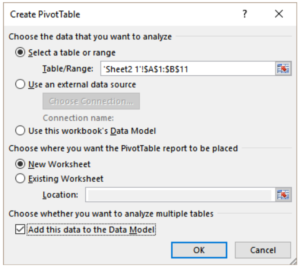
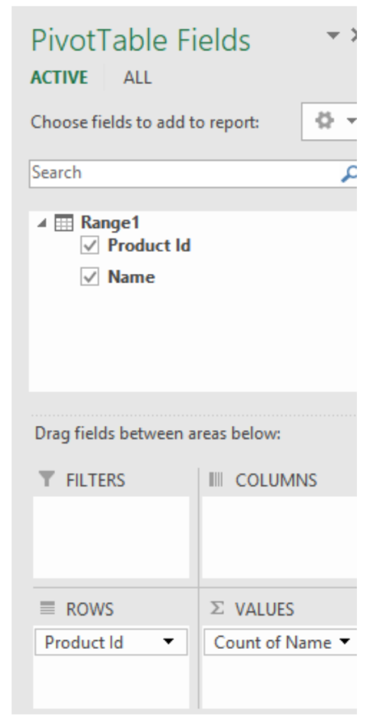
- Drag the Product ID field to Rows, Names field to Values in the PivotTable Fields.
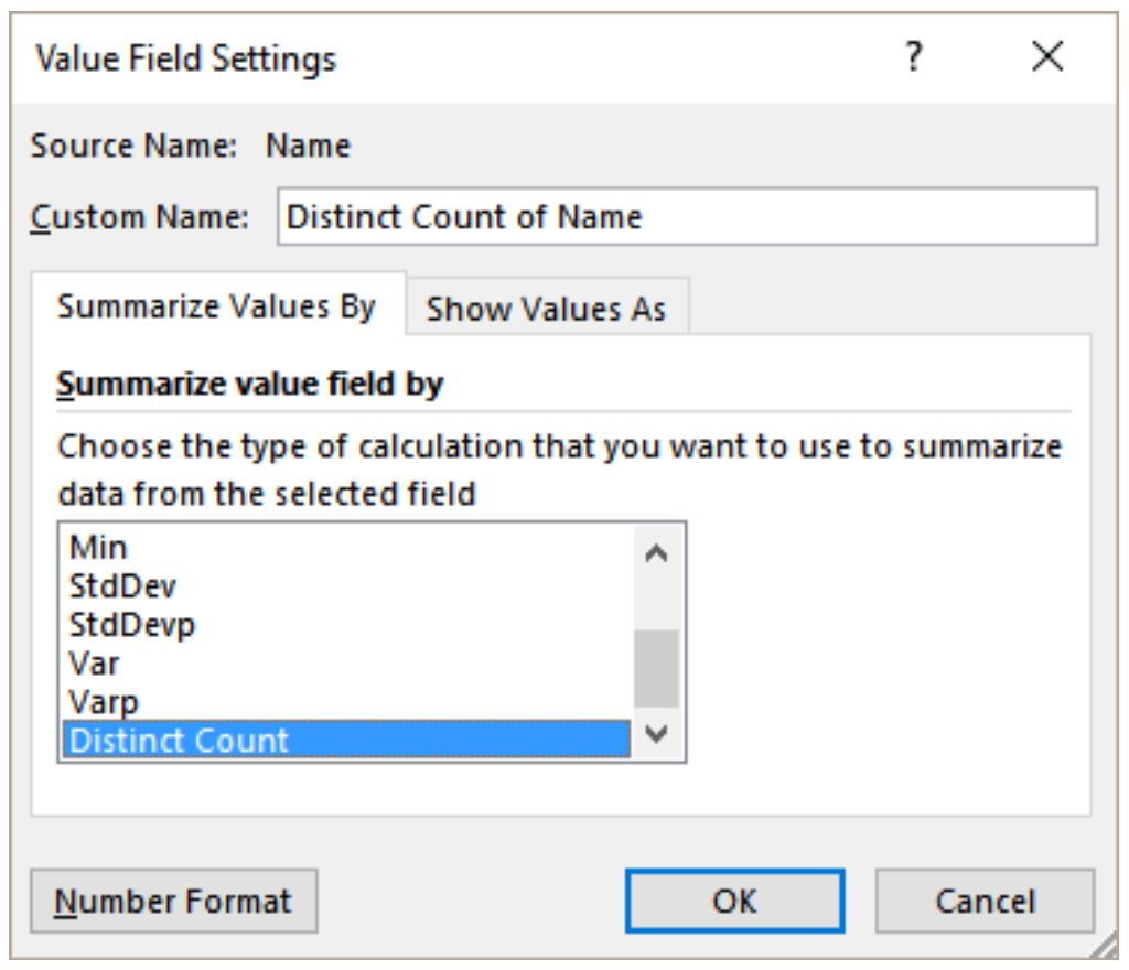
- Right-click on any value in column B. Go to Value Field Settings. In the Summarize Values By tab, go to Summarize Value field by and set it to Distinct Count.
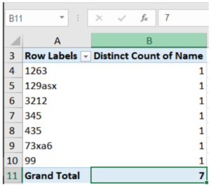
This will show the distinct count 7 in cell B11.
Still need some help with Excel formatting or have other questions about Excel? Connect with a live Excel expert here for some 1 on 1 help. Your first session is always free.
Do you want to count distinct values in a list in Excel?
When performing any data analysis in Excel you will often want to know the number of distinct items in a column. This statistic can give you a useful overview of the data and help you spot errors or inconsistencies.
This post will show you all the ways you can count the number of distinct items in your list. Get your copy of the example workbook in this post to follow along.
Distinct vs Unique
The terms unique and distinct are often incorrectly interchanged liberally. There is a big difference between these terms.
Distinct means values that are different. The distinct values from this list {A, B, B, C} are {A, B, C}. The count in this case will be 3.
Unique means values that only appear once. The unique values from the list {A, B, B, C} are {A, C}. The count in this case will be 2.
💡 Tip: Check out this post if you are actually looking for a count of unique items.
Count Distinct Values with the COUNTIFS Function
The first way to count the unique values in a range is with the COUNTIFS function.
The COUNTIFS function allows you to count values based on one or more criteria.
= SUM ( 1 / COUNTIFS ( B5:B14, B5:B14 ) )The above formula will count the number of distinct items from the list of values in the range B5:B14.
The COUNTIFS function is used to see how many times each value appears in the list. When you invert this count you get a fractional value that will add up to 1 for each distinct value in the list.
The SUM function then adds all these fractions up and the total is the number of distinct items in the list.
💡 Tip: If you are working with an older version of Excel that doesn’t support array formulas, then you will need to enter this formula with Ctrl + Shift + Enter.
Count Distinct Values with the UNIQUE Function
Another formula approach to counting the number of distinct items from the list is with dynamic array functions.
However, these are only available in Excel for Microsoft 365.
= COUNTA ( UNIQUE ( B5:B14 ) )The above formula will return the count of all distinct items from the list in B5:B14.
The UNIQUE function returns all the distinct values from the list. The number of items in the distinct list is then counted using the COUNTA function.
Count Distinct Values with Advanced Filters
Advanced Filters is a feature that allows you to add complex logic based on multiple fields to filter your lists.
This can also be used to filter the distinct values in your list.
You can then use a SUBTOTAL function to count only the visible items in your filtered list.
Here’s how to count the distinct items with the advanced filters.
= SUBTOTAL ( 103, B5:B14 )- Add the above SUBTOTAL function to the range you want to count values from. The
103argument tells the SUBTOTAL function to only count the visible cells in a range.
- Select the column of data in which you want to count distinct values.
- Go to the Data tab.
- Click on the Advanced command in the Sort and Filter section of the ribbon.
This will open the Advanced Filter menu.
- Select the Filter the list in place option from the Action section.
- The List range should be the range of values previously selected in step 2. You can update this if needed.
- Check the Unique records only option. Even though it says unique, it will actually return the distinct values in the filter.
- Press the OK button.
The list is filtered to hide all the repeated values and the SUBTOTAL will then only count the distinct items in the list.
Count Distinct Values with a Pivot Table
You can get a list of distinct values from a pivot table.
When you summarize your data by rows in a pivot table, the rows area will show only the distinct items. You can then count these with the status bar statistics or the COUNTA function.
You will first need to create a pivot table with the data that you want to get a distinct count.
- Select the data.
- Go to the Insert tab.
- Click on the PivotTable command.
This opens the PivotTable from table or range menu where you can select where you want to place the new pivot table.
- Choose the location for your new pivot table.
- Press the OK button.
This will create a new blank pivot table. When you select any cell inside this pivot table, you will see the PivotTable Fields list appear on the right side of the workbook.
- Drag the field from which you want to count distinct items into the Rows area of the pivot table.
This creates a list of distinct items in the pivot table. Now you can select these items and the count will be displayed in the status bar area.
Count Distinct Values with the Pivot Table Data Model
While using a pivot table will get you the list of distinct items from your data, it’s not ideal for counting the results. There is an additional step of selecting the items and getting the count in the status bar.
But there is a way to use a pivot table and return the count of distinct items inside the Values area of the pivot table.
When you use the pivot table data model feature, it will reveal an extra summary type in the field settings that will count distinct values.
You will insert the pivot table as before, but there is an extra step during the process.
- Check the Add this data to the Data Model option in the PivotTable from table or range menu.
- Drag the field into the Values area. It should default to a count.
- Left-click on the field.
- Select Value Field Settings from the menu options.
This opens the Value Field Settings menu.
- Go to the Summarize Values By tab.
- Choose the Distinct Count option in the Summarize value field by list. This option only appears when the data has been added to the data model.
- Press the OK button.
That’s it! The distinct count of items now appears in your pivot table.
This is much more versatile as you can now get the distinct count within another categorical grouping by adding a field into the Rows area.
For example, each value in the pivot table is now a distinct count of the car model based on the make.
Count Distinct Values Remove Duplicates
The Remove Duplicates feature will allow you to get rid of any repeated values in your list.
You can then count the results to get a distinct count of items.
- Select the range of items to count.
- Go to the Data tab.
- Click on the Remove Duplicates command.
This will open the Remove Duplicates menu.
- Select a single column in the list of Columns.
- Press the OK button.
This will remove the duplicates in your list and a popup will show telling you how many items were removed and how many remain. This is the number of distinct items from the list!
📝 Note: This will change the data, so be sure to only perform this command on a copy of your source data so you don’t lose the original.
Count Distinct Values with Power Query Column Distribution
Power Query is a great tool for importing and transforming data.
When building your queries, it will even show you useful summary statistics about the data in the column distribution view. This includes a distinct count.
You will first need to load your data into the Power Query editor to see these features.
- Select the data.
- Go to the Data tab.
- Select the From Table/Range query option.
This will open the Power Query editor and you might already see the column distribution feature with the distinct count.
If you don’t see this, you can enable it from the View tab in the editor.
- Go to the View tab.
- Check the Column distribution option in the Data Preview section.
💡 Tip: Hover your mouse cursor over the counts and you’ll see a percentage distribution!
Count Distinct Values with Power Query Transform Tab
The column distribution feature is handy for a quick overview of the data, but you might want to get this value back into Excel from your Power Query.
This is also possible.
- Select the column you want to count.
- Go to the Transform tab.
- Click on the Statistics command in the Number Column section.
- Select the Count Distinct Values option from the menu.
This returns a sing scalar value from your column which is the count of the distinct items in that column.
You can load this back into Excel and it will load into a single column and single row table. Go to the Home tab and click on the Close and Load button.
Count Distinct Values with VBA
There is no prebuilt function in Excel that will count the number of distinct items in a range.
However, you can build your own custom VBA function for this purpose.
Press the Alt + F11 keyboard shortcut to open the visual basic editor. This is where you can place the code for your user-defined function.
Go to the Insert menu and select the Module option to create a new module for your code.
Function COUNTDISTINCTVALUES(rng As Range) As Integer
Application.Volatile
Dim c As Variant
Dim distinctValues As New Collection

On Error Resume Next
For Each c In rng
    If Not (IsEmpty(c)) Then
        distinctValues.Add c, CStr(c)
    End If
Next c
COUNTDISTINCTVALUES = distinctValues.Count
End Function
Copy and paste the above code into the module.
This code will create a new function named COUNTDISTINCTVALUES which can be used anywhere in the workbook just like any other function.
The will loop through each cell in the range it is passed. If the cell is not empty, then the value in the cell is added to a collection object.
Collections will only allow distinct values to be added, so the end result will be a collection of only the distinct values from your range.
The count of the items in the collection is then returned as the function output!
= COUNTDISTINCTVALUES ( B3:B12 )The above formula will then return the distinct count of the values in the range B3:B12.
Count Distinct Values with Office Scripts
Office scripts are another way to get a distinct count for a selected range.
You can create a script that will count distinct items in the active range.
Go to the Automate tab and select the New Script option.
This will open the Code Editor.
function main(workbook: ExcelScript.Workbook) {
    let rng = workbook.getSelectedRange();
    let rngValues = rng.getValues();
    let arrayValues = rngValues.reduce((a, value) => a.concat(value), []);
    let distinctValues = new Set(arrayValues);
    console.log(distinctValues.size);
};
Add the above code and press the Save script button.
This code gets the values from the selected range in the sheet. It will then convert this to a one-dimensional array of values with the reduce function.
This 1D array is then added to a Set. Sets also have the property that they only allow distinct values, so the distinctValues set will only have the distinct values from the selected range.
The number of items is counted with the size and this is returned to the console log to give you the count of distinct values.
Conclusions
There are several options for counting the distinct number of items in a list.
Formulas solutions are great for dynamic live results directly in your sheet. Other features such as advanced filters or remove duplicates are only suited for one-time uses.
If you’re already using Pivot Tables or Power Query in your data processing, then getting the distinct count in those tools is a natural choice.
For any other situation, or as part of a larger automated process, the custom VBA or Office Scripts code solutions might be the best.
Did you know any of these methods? Let me know in the comments!
About the Author
John is a Microsoft MVP and qualified actuary with over 15 years of experience. He has worked in a variety of industries, including insurance, ad tech, and most recently Power Platform consulting. He is a keen problem solver and has a passion for using technology to make businesses more efficient.
![]()
When you create a pivot table to summarize data, Excel automatically creates sums and counts for the fields that you add to the Values area. In addition, you might want to see a distinct count (unique count) for some fields, such as:
- The number of distinct salespeople who made sales in each region
- The count of unique products that were sold in each store
Normal Pivot Tables
For a normal pivot table, there isn’t a built-in distinct count feature in a normal pivot table. However, in Excel 2013 and later versions, you can use a simple trick, described below, to show a distinct count for a field.
For older versions of Excel, try one of the following methods:
- In Excel 2010, use a technique to “Pivot the Pivot table”.
- In Excel 2007 and earlier versions, add a new column to the source data, and Use CountIf.
Add to Data Model – Excel 2013 and Later
In Excel 2013, if you add a pivot table’s source data to the workbook’s Data Model, it is easy to create a distinct count in Excel pivot table.
NOTE: This technique creates an OLAP-based pivot table, which has some limitations, such as no ability to add calculated fields or calculated items. If you need the restricted features, try the “Pivot the Pivot” method instead.

The Sample Data
In this example, there are 4999 records that show product sales, with the region and salesperson name. The first few records are shown in the screen shot below.
You can download the sample workbook from my Contextures website. On the Pivot Table Unique Count page, go to the Download section, and click the link.

Create the Pivot Table
First, to create a pivot table that will show a distinct count, follow these steps:
- Select a cell in the source data table.
- At the bottom of the Create PivotTable dialog box, add a check mark to “Add this data to the Data Model”
- Click OK

Set up the Pivot Table Layout
To set up the pivot table layout, follow these steps:
- In the pivot table, add Region to the Row area.
- Add these 3 fields to the Values area — Person, Units, Value
- The Person field contains text, so it defaults to Count of Person. The count shows the total number of transactions in each region, not a unique count of salespeople

Show a Distinct Count
To get a unique count (distinct count) of salespeople in each region, follow these steps:
- Right-click one of the values in the Person field
- Click Value Field Settings

- In the Summarize Value Field By list, scroll to the bottom, and click Distinct Count, then click OK

The Person field changes, and instead of showing the total count of transactions, it shows a distinct count of salespeople names.

Distinct Count in Excel Pivot Table Workbook
To download the sample workbook, go to the Pivot Table Unique Count page, on my Contextures website. On that page, go to the Download section, and click the link.
That page also has instructions for calculating a unique count in older versions of Excel.
_________________________
Excel Distinct Count or Unique Count. Pivot tables will offer a distinct count, if you check one tiny box as you create the pivot table.
Here is an annoyance with pivot tables. Drag the Customer column from the Data table to the VALUES area. The field says Count of Customer, but it is really a count of how many invoices belong to each sector. What if you really want to see how many unique customers belong to each sector?
Select a cell in the Count of Customer column. Click Field Settings. At first, the Summarize Values By looks like the same Sum, Average, and Count that you’ve always had. But scroll down to the bottom. Because the pivot table is based on the Data Model, you now have Distinct Count.
After you select Distinct Count, the pivot table shows a distinct count of customers for each sector. This was very hard to do in regular pivot tables.
To join two tables in Excel 2010, you have to download the free Power Pivot add-in from Microsoft. Once you have that installed, here are the extra steps to get your data into Power Pivot:
When it comes time to create relationships, you have only one button called Create. Excel 2010 will attempt to AutoDetect relationships first. In this simple example, it will get the relationship correct.
Thanks to Colin Michael and Alejandro Quiceno for suggesting Power Pivot in general.
Learn Excel from MrExcel podcast, episode
2015 — Distinct Count!
Alright, all the tips in this book are
going to be podcast, check out this playlist for the whole set!
OK, so today we have to create a report
that shows how many customers are in each sector, and a regular Pivot table CANNOT
do this. So Insert PivotTable will put sectors down the left-hand side, and
then ask for the count of Customer, and it says it’s giving us the count of
Customer. But this isn’t the count of Customer, this is how many records there
are, alright, we don’t have 563 customers, completely, completely useless. But
check this out, amazingly easy to solve this, yesterday’s podcast we talked
about using the Data Model to join 2 tables together. Today I just have one
table, there’s, you know, you wouldn’t think there’s any reason to use the data
model, except for this, so choose the box “Add this data to the Data Model”.
By the way, this is brand new in Excel
2013, so you need 13 or 16, if you’re stuck on a Mac or back in Excel 2010,
I’ll show you the old solution here at the end. Click OK, build the exact same
report, sectors down the left-hand side, count of Customer, an exact same wrong
answer, but here’s the difference. When we come into Field Settings see, it
looks the same, Sum, Count, Average, Max, Min, there’s a few missing, and at
the very bottom there’s a new one called Distinct Count. Wow, that is something
that has been so hard to do in old versions of Excel, in fact let me show you
how we used to do it in Excel 2010.
So here’s the data, you would have to come
out and do a COUNTIF, count how many times Vertex42 appears in column D, and it
appears there are 6 times. So then the Distinct Count is =1 divided by that, alright,
see what we’re doing, if there’s six records with Vertex42, we’re giving each
of them 1/6 or 0.16611, and when we add all that up, that will get us to 1,
right? There’s 5 records here, each gets 1/5 or 20%, add all those up, each of
those gets us to 1. So back in Excel 2010 or 7 or 3 or wherever you are, you
don’t have the Data Model, so you add those extra fields there, Sector, and
then Distinct Count. This was so much more difficult than the new way, so I
certainly appreciate the data model for this one. Well this tip, and a lot more
in the book, click the “i” on the top-right hand corner, you can buy the book,
$25 in print, $10 for an e-book, it’s cheap!
In yesterday’s podcast, 2014, we talked
about the Data Model for joining tables, another benefit is the ability to do a
distinct count. Regular Pivot table cannot count customers per sector, add the
data to the Data Model, and you have Distinct Count available. Before Excel
2013, you do 1/COUNTIF in the original data, and of course, if you want to do
distinct count for something else, you might have to change that formula,
really, really frustrating. Beautiful, beautiful side benefit of the whole
Power Pivot engine!