Display text in if excel

IF function

The IF function is one of the most popular functions in Excel, and it allows you to make logical comparisons between a value and what you expect.

So an IF statement can have two results. The first result is if your comparison is True, the second if your comparison is False.

For example, =IF(C2=”Yes”,1,2) says IF(C2 = Yes, then return a 1, otherwise return a 2).

Use the IF function, one of the logical functions, to return one value if a condition is true and another value if it’s false.

IF(logical_test, value_if_true, [value_if_false])

For example:

• =IF(A2>B2,»Over Budget»,»OK»)

• =IF(A2=B2,B4-A4,»»)

Argument name	Description
logical_test    (required)	The condition you want to test.
value_if_true    (required)	The value that you want returned if the result of logical_test is TRUE.
value_if_false    (optional)	The value that you want returned if the result of logical_test is FALSE.

Simple IF examples

• =IF(C2=”Yes”,1,2)

In the above example, cell D2 says: IF(C2 = Yes, then return a 1, otherwise return a 2)

• =IF(C2=1,”Yes”,”No”)

In this example, the formula in cell D2 says: IF(C2 = 1, then return Yes, otherwise return No)As you see, the IF function can be used to evaluate both text and values. It can also be used to evaluate errors. You are not limited to only checking if one thing is equal to another and returning a single result, you can also use mathematical operators and perform additional calculations depending on your criteria. You can also nest multiple IF functions together in order to perform multiple comparisons.

• =IF(C2>B2,”Over Budget”,”Within Budget”)

In the above example, the IF function in D2 is saying IF(C2 Is Greater Than B2, then return “Over Budget”, otherwise return “Within Budget”)

• =IF(C2>B2,C2-B2,0)

In the above illustration, instead of returning a text result, we are going to return a mathematical calculation. So the formula in E2 is saying IF(Actual is Greater than Budgeted, then Subtract the Budgeted amount from the Actual amount, otherwise return nothing).

• =IF(E7=”Yes”,F5*0.0825,0)

In this example, the formula in F7 is saying IF(E7 = “Yes”, then calculate the Total Amount in F5 * 8.25%, otherwise no Sales Tax is due so return 0)

Note: If you are going to use text in formulas, you need to wrap the text in quotes (e.g. “Text”). The only exception to that is using TRUE or FALSE, which Excel automatically understands.

Common problems

Problem	What went wrong
0 (zero) in cell	There was no argument for either value_if_true or value_if_False arguments. To see the right value returned, add argument text to the two arguments, or add TRUE or FALSE to the argument.
#NAME? in cell	This usually means that the formula is misspelled.

Need more help?

You can always ask an expert in the Excel Tech Community or get support in the Answers community.

See Also

IF function — nested formulas and avoiding pitfalls

IFS function

Using IF with AND, OR and NOT functions

COUNTIF function

How to avoid broken formulas

Overview of formulas in Excel

Normally, If you want to write an IF formula for text values in combining with the below two logical operators in excel, such as: “equal to” or “not equal to”.

Excel IF function check if a cell contains text(case-insensitive)

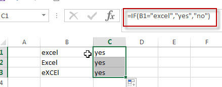
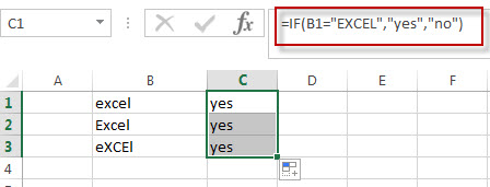
By default, IF function is case-insensitive in excel. It means that the logical text for text values will do not recognize case in the IF formulas. For example, the following two IF formulas will get the same results when checking the text values in cells.

=IF(B1="excel","yes","no")
=IF(B1="EXCEl","yes","no")

The IF formula will check the values of cell B1 if it is equal to “excel” word, If it is TRUE, then return “yes”, otherwise return “no”. And the logical test in the above IF formula will check the text values in the logical_test argument, whatever the logical_test values are “Excel”, “eXcel”, or “EXCEL”, the IF formula don’t care about that if the text values is in lowercase or uppercase, It will get the same results at last.

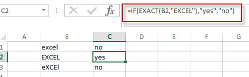
Excel IF function check if a cell contains text (case-sensitive)

If you want to check text values in cells using IF formula in excel (case-sensitive), then you need to create a case-sensitive logical test and then you can use IF function in combination with EXACT function to compare two text values. So if those two text values are exactly the same, then return TRUE. Otherwise return FALSE.

So we can write down the following IF formula combining with EXACT function:

=IF(EXACT(B1,"excel"),"yes","no")

Excel IF function check if part of cell matches specific text

If you want to check if part of text values in cell matches the specific text rather than exact match, to achieve this logic text, you can use IF function in combination with ISNUMBER and SEARCH Function in excel.

Both ISNUMBER and SEARCH functions are case-insensitive in excel.

=IF(ISNUMBER(SEARCH("x",B1)),"good","bad")

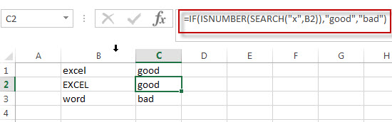
For above the IF formula, it will Check to see if B1 contain the letter x.

Also, we can use FIND function to replace the SEARCH function in the above IF formula. It will return the same results.

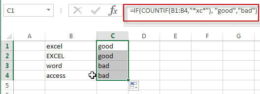
 Excel IF function with Wildcards text value

If you wan to use wildcard charcter in an IF formula, for example, if any of the values in column B contains “*xc*”, then return “good”, others return “bad”. You can not directly use the wildcard characters in IF formula, and we can use IF function in combination with COUNTIF function. Let’s see the following IF formula:

=IF(COUNTIF(B1:B4,"*xc*"), "good","bad")

---

• Excel IF Function With Numbers
  If you want to check if a cell values is between two values or checking for the range of numbers or multiple values in cells, at this time, we need to use AND or OR logical function in combination with the logical operator and IF function…

• Excel EXACT function
  The Excel SEARCH function returns the number of the starting location of a substring in a text string.The syntax of the EXACT function is as below:= EXACT (text1,text2)…
• Excel COUNTIF function
  The Excel COUNTIF function will count the number of cells in a range that meet a given criteria.= COUNTIF (range, criteria) …
  
• Excel ISNUMBER function
  The Excel ISNUMBER function returns TRUE if the value in a cell is a numeric value, otherwise it will return FALSE.
• Excel IF function
  The Excel IF function perform a logical test to return one value if the condition is TRUE and return another value if the condition is FALSE….
• Excel SEARCH function
  The Excel SEARCH function returns the number of the starting location of a substring in a text string.…

The logical IF statement in Excel is used for the recording of certain conditions. It compares the number and / or text, function, etc. of the formula when the values correspond to the set parameters, and then there is one record, when do not respond — another.

Logic functions — it is a very simple and effective tool that is often used in practice. Let us consider it in details by examples.



The syntax of the function «IF» with one condition

The operation syntax in Excel is the structure of the functions necessary for its operation data.

=IF(boolean;value_if_TRUE;value_if_FALSE)

Let us consider the function syntax:

• Boolean – what the operator checks (text or numeric data cell).
• Value_if_TRUE – what will appear in the cell when the text or numbers correspond to a predetermined condition (true).
• Value_if_FALSE – what appears in the box when the text or the number does not meet the predetermined condition (false).

Example:

Logical IF functions.

The operator checks the A1 cell and compares it to 20. This is a «Boolean». When the contents of the column is more than 20, there is a true legend «greater 20». In the other case it’s «less or equal 20».

Attention! The words in the formula need to be quoted. For Excel to understand that you want to display text values.

Here is one more example. To gain admission to the exam, a group of students must successfully pass a test. The results are listed in a table with columns: a list of students, a credit, an exam.

The statement IF should check not the digital data type but the text. Therefore, we prescribed in the formula В2= «done» We take the quotes for the program to recognize the text correctly.



The function IF in Excel with multiple conditions

Usually one condition for the logic function is not enough. If you need to consider several options for decision-making, spread operators’ IF into each other. Thus, we get several functions IF in Excel.

The syntax is as follows:

Here the operator checks the two parameters. If the first condition is true, the formula returns the first argument is the truth. False — the operator checks the second condition.

Examples of a few conditions of the function IF in Excel:

It’s a table for the analysis of the progress. The student received 5 points:

• А – excellent;
• В – above average or superior work;
• C – satisfactory;
• D – a passing grade;
• E – completely unsatisfactory.

IF statement checks two conditions: the equality of value in the cells.

In this example, we have added a third condition, which implies the presence of another report card and «twos». The principle of the operator is the same.

Enhanced functionality with the help of the operators «AND» and «OR»

When you need to check out a few of the true conditions you use the function И. The point is: IF A = 1 AND A = 2 THEN meaning в ELSE meaning с.

OR function checks the condition 1 or condition 2. As soon as at least one condition is true, the result is true. The point is: IF A = 1 OR A = 2 THEN value B ELSE value C.

Functions AND & OR can check up to 30 conditions.

An example of using the operator AND:

It’s the example of using the logical operator OR.

How to compare data in two tables

Users often need to compare the two spreadsheets in an Excel to match. Examples of the «life»: compare the prices of goods in different bringing, to compare balances (accounting reports) in a few months, the progress of pupils (students) of different classes, in different quarters, etc.

To compare the two tables in Excel, you can use the COUNTIFS statement. Consider the order of application functions.

For example, consider the two tables with the specifications of various food processors. We planned allocation of color differences. This problem in Excel solves the conditional formatting.

Baseline data (tables, which will work with):

Select the first table. Conditional Formatting — create a rule — use a formula to determine the formatted cells:

In the formula bar write: = COUNTIFS (comparable range; first cell of first table)=0. Comparing range is in the second table.

To drive the formula into the range, just select it first cell and the last. «= 0» means the search for the exact command (not approximate) values.

Choose the format and establish what changes in the cell formula in compliance. It’s better to do a color fill.

Select the second table. Conditional Formatting — create a rule — use the formula. Use the same operator (COUNTIFS). For the second table formula:

Download all examples in Excel

Now it is easy to compare the characteristics of the data in the table.

A1 and less than 10, return «OK». Otherwise, return nothing («»).

To return B1+10 when A1 is «red» or «blue» you can use the OR function like this:

Translation: if A1 is red or blue, return B1+10, otherwise return B1.

Translation: if A1 is NOT red, return B1+10, otherwise return B1.

IF cell contains specific text

Because the IF function does not support wildcards, it is not obvious how to configure IF to check for a specific substring in a cell. A common approach is to combine the ISNUMBER function and the SEARCH function to create a logical test like this:

For example, to check for the substring «xyz» in cell A1, you can use a formula like this:

Источник

Excel IF statement with multiple conditions

by Svetlana Cheusheva, updated on February 7, 2023

The tutorial shows how to create multiple IF statements in Excel with AND as well as OR logic. Also, you will learn how to use IF together with other Excel functions.

In the first part of our Excel IF tutorial, we looked at how to construct a simple IF statement with one condition for text, numbers, dates, blanks and non-blanks. For powerful data analysis, however, you may often need to evaluate multiple conditions at a time. The below formula examples will show you the most effective ways to do this.

How to use IF function with multiple conditions

In essence, there are two types of the IF formula with multiple criteria based on the AND / OR logic. Consequently, in the logical test of your IF formula, you should use one of these functions:

• AND function — returns TRUE if all the conditions are met; FALSE otherwise.
• OR function — returns TRUE if any single condition is met; FALSE otherwise.

To better illustrate the point, let’s investigate some real-life formulas examples.

Excel IF statement with multiple conditions (AND logic)

The generic formula of Excel IF with two or more conditions is this:

Translated into a human language, the formula says: If condition 1 is true AND condition 2 is true, return value_if_true; else return value_if_false.

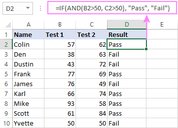
Suppose you have a table listing the scores of two tests in columns B and C. To pass the final exam, a student must have both scores greater than 50.

For the logical test, you use the following AND statement: AND(B2>50, C2>50)

If both conditions are true, the formula will return «Pass»; if any condition is false — «Fail».

=IF(AND(B2>50, B2>50), «Pass», «Fail»)

Easy, isn’t it? The screenshot below proves that our Excel IF /AND formula works right:

In a similar manner, you can use the Excel IF function with multiple text conditions.

For instance, to output «Good» if both B2 and C2 are greater than 50, «Bad» otherwise, the formula is:

=IF(AND(B2=»pass», C2=»pass»), «Good!», «Bad»)

Important note! The AND function checks all the conditions, even if the already tested one(s) evaluated to FALSE. Such behavior is a bit unusual since in most of programming languages, subsequent conditions are not tested if any of the previous tests has returned FALSE.

In practice, a seemingly correct IF statement may result in an error because of this specificity. For example, the below formula would return #DIV/0! («divide by zero» error) if cell A2 is equal to 0:

The avoid this, you should use a nested IF function:

=IF(A2<>0, IF((1/A2)>0.5, «Good», «Bad»), «Bad»)

For more information, please see IF AND formula in Excel.

Excel IF function with multiple conditions (OR logic)

To do one thing if any condition is met, otherwise do something else, use this combination of the IF and OR functions:

The difference from the IF / AND formula discussed above is that Excel returns TRUE if any of the specified conditions is true.

So, if in the previous formula, we use OR instead of AND:

=IF(OR(B2>50, B2>50), «Pass», «Fail»)

Then anyone who has more than 50 points in either exam will get «Pass» in column D. With such conditions, our students have a better chance to pass the final exam (Yvette being particularly unlucky failing by just 1 point 🙂

Tip. In case you are creating a multiple IF statement with text and testing a value in one cell with the OR logic (i.e. a cell can be «this» or «that»), then you can build a more compact formula using an array constant.

For example, to mark a sale as «closed» if cell B2 is either «delivered» or «paid», the formula is:

More formula examples can be found in Excel IF OR function.

IF with multiple AND & OR statements

If your task requires evaluating several sets of multiple conditions, you will have to utilize both AND & OR functions at a time.

In our sample table, suppose you have the following criteria for checking the exam results:

• Condition 1: exam1>50 and exam2>50
• Condition 2: exam1>40 and exam2>60

If either of the conditions is met, the final exam is deemed passed.

At first sight, the formula seems a little tricky, but in fact it is not! You just express each of the above conditions as an AND statement and nest them in the OR function (since it’s not necessary to meet both conditions, either will suffice):

OR(AND(B2>50, C2>50), AND(B2>40, C2>60)

Then, use the OR function for the logical test of IF and supply the desired value_if_true and value_if_false values. As the result, you get the following IF formula with multiple AND / OR conditions:

=IF(OR(AND(B2>50, C2>50), AND(B2>40, C2>60), «Pass», «Fail»)

The screenshot below indicates that we’ve done the formula right:

Naturally, you are not limited to using only two AND/OR functions in your IF formulas. You can use as many of them as your business logic requires, provided that:

• In Excel 2007 and higher, you have no more than 255 arguments, and the total length of the IF formula does not exceed 8,192 characters.
• In Excel 2003 and lower, there are no more than 30 arguments, and the total length of your IF formula does not exceed 1,024 characters.

Nested IF statement to check multiple logical tests

If you want to evaluate multiple logical tests within a single formula, then you can nest several functions one into another. Such functions are called nested IF functions. They prove particularly useful when you wish to return different values depending on the logical tests’ results.

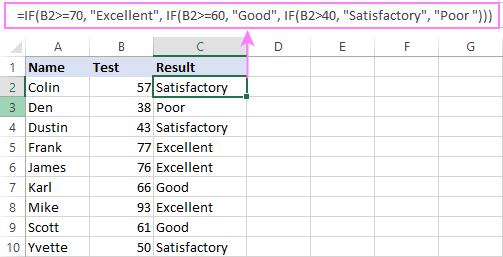
Here’s a typical example: suppose you want to qualify the students’ achievements as «Good«, «Satisfactory» and «Poor» based on the following scores:

• Good: 60 or more (>=60)
• Satisfactory: between 40 and 60 (>40 and =IF(B2>=60, «Good», IF(B2>40, «Satisfactory», «Poor»))

Naturally, you can nest more functions if needed (up to 64 in modern versions).

Excel IF array formula with multiple conditions

Another way to get an Excel IF to test multiple conditions is by using an array formula.

To evaluate conditions with the AND logic, use the asterisk:

To test conditions with the OR logic, use the plus sign:

To complete an array formula correctly, press the Ctrl + Shift + Enter keys together. In Excel 365 and Excel 2021, this also works as a regular formula due to support for dynamic arrays.

For example, to get «Pass» if both B2 and C2 are greater than 50, the formula is:

=IF((B2>50) * (C2>50), «Pass», «Fail»)

In my Excel 365, a normal formula works just fine (as you can see in the screenshots above). In Excel 2019 and lower, remember to make it an array formula by using the Ctrl + Shift + Enter shortcut.

To evaluate multiple conditions with the OR logic, the formula is:

=IF((B2>50) + (C2>50), «Pass», «Fail»)

Using IF together with other functions

This section explains how to use IF in combination with other Excel functions and what benefits this gives to you.

Example 1. If #N/A error in VLOOKUP

When VLOOKUP or other lookup function cannot find something, it returns a #N/A error. To make your tables look nicer, you can return zero, blank, or specific text if #N/A. For this, use this generic formula:

If the lookup value in E1 is not found, the formula returns zero.

=IF(ISNA(VLOOKUP(E1, A2:B10, 2,FALSE )), 0, VLOOKUP(E1, A2:B10, 2, FALSE))

If #N/A return blank:

If the lookup value is not found, the formula returns nothing (an empty string).

=IF(ISNA(VLOOKUP(E1, A2:B10, 2,FALSE )), «», VLOOKUP(E1, A2:B10, 2, FALSE))

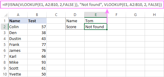
If #N/A return certain text:

If the lookup value is not found, the formula returns specific text.

=IF(ISNA(VLOOKUP(E1, A2:B10, 2,FALSE )), «Not found», VLOOKUP(E1, A2:B10, 2, FALSE))

For more formula examples, please see VLOOKUP with IF statement in Excel.

Example 2. IF with SUM, AVERAGE, MIN and MAX functions

To sum cell values based on certain criteria, Excel provides the SUMIF and SUMIFS functions.

In some situations, your business logic may require including the SUM function in the logical test of IF. For example, to return different text labels depending on the sum of the values in B2 and C2, the formula is:

=IF(SUM(B2:C2)>130, «Good», IF(SUM(B2:C2)>110, «Satisfactory», «Poor»))

If the sum is greater than 130, the result is «good»; if greater than 110 – «satisfactory’, if 110 or lower – «poor».

In a similar fashion, you can embed the AVERAGE function in the logical test of IF and return different labels based on the average score:

=IF(AVERAGE(B2:C2)>65, «Good», IF(AVERAGE(B2:C2)>55, «Satisfactory», «Poor»))

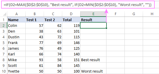
Assuming the total score is in column D, you can identify the highest and lowest values with the help of the MAX and MIN functions:

=IF(D2=MAX($D$2:$D$10), «Best result», «»)

=IF(D2=MAX($D$2:$D$10), «Best result», «»)

To have both labels in one column, nest the above functions one into another:

=IF(D2=MAX($D$2:$D$10), «Best result», IF(D2=MIN($D$2:$D$10), «Worst result», «»))

Likewise, you can use IF together with your custom functions. For example, you can combine it with GetCellColor or GetCellFontColor to return different results based on a cell color.

In addition, Excel provides a number of functions to calculate data based on conditions. For detailed formula examples, please check out the following tutorials:

• COUNTIF — count cells that meet a condition
• COUNTIFS — count cells with multiple criteria
• SUMIF — conditionally sum cells
• SUMIFS — sum cells with multiple criteria

Example 3. IF with ISNUMBER, ISTEXT and ISBLANK

To identify text, numbers and blank cells, Microsoft Excel provides special functions such as ISTEXT, ISNUMBER and ISBLANK. By placing them in the logical tests of three nested IF statements, you can identify all different data types in one go:

=IF(ISTEXT(A2), «Text», IF(ISNUMBER(A2), «Number», IF(ISBLANK(A2), «Blank», «»)))

Example 4. IF and CONCATENATE

To output the result of IF and some text into one cell, use the CONCATENATE or CONCAT (in Excel 2016 — 365) and IF functions together. For example:

=CONCATENATE(«You performed «, IF(B1>100,»fantastic!», IF(B1>50, «well», «poor»)))

=CONCAT(«You performed «, IF(B1>100,»fantastic!», IF(B1>50, «well», «poor»)))

Looking at the screenshot below, you’ll hardly need any explanation of what the formula does:

IF ISERROR / ISNA formula in Excel

The modern versions of Excel have special functions to trap errors and replace them with another calculation or predefined value — IFERROR (in Excel 2007 and later) and IFNA (in Excel 2013 and later). In earlier Excel versions, you can use the IF ISERROR and IF ISNA combinations instead.

The difference is that IFERROR and ISERROR handle all possible Excel errors, including #VALUE!, #N/A, #NAME?, #REF!, #NUM!, #DIV/0!, and #NULL!. While IFNA and ISNA specialize solely in #N/A errors.

For example, to replace the «divide by zero» error (#DIV/0!) with your custom text, you can use the following formula:

=IF(ISERROR(A2/B2), «N/A», A2/B2)

And that’s all I have to say about using the IF function in Excel. I thank you for reading and hope to see you on our blog next week!

Источник

Adblock
detector

The IF function runs a logical test and returns one value for a TRUE result, and another value for a FALSE result. The result from IF can be a value, a cell reference, or even another formula. By combining the IF function with other logical functions like AND and OR, you can test more than one condition at a time.

Syntax

The generic syntax for the IF function looks like this:

=IF(logical_test,[value_if_true],[value_if_false])

The first argument, logical_test, is typically an expression that returns either TRUE or FALSE. The second argument, value_if_true, is the value to return when logical_test is TRUE. The last argument, value_if_false, is the value to return when logical_test is FALSE. Both value_if_true and value_if_false are optional, but you must provide one or the other. For example, if cell A1 contains 80, then:

=IF(A1>75,TRUE) // returns TRUE
=IF(A1>75,"OK") // returns "OK"
=IF(A1>85,"OK") // returns FALSE
=IF(A1>75,10,0) // returns 10
=IF(A1>85,10,0) // returns 0
=IF(A1>75,"Yes","No") // returns "Yes"
=IF(A1>85,"Yes","No") // returns "No"

Notice that text values like «OK», «Yes», «No», etc. must be enclosed in double quotes («»). However, numeric values should not be enclosed in quotes.

Logical tests

The IF function supports logical operators (>,<,<>,=) when creating logical tests. Most commonly, the logical_test in IF is a complete logical expression that will evaluate to TRUE or FALSE. The table below shows some common examples:

Goal	Logical test
If A1 is greater than 75	A1>75
If A1 equals 100	A1=100
If A1 is less than or equal to 100	A1<=100
If A1 equals «Red»	A1=»red»
If A1 is not equal to «Red»	A1<>»red»
If A1 is less than B1	A1<B1
If A1 is empty	A1=»»
If A1 is not empty	A1<>»»
If A1 is less than current date	A1<TODAY()

Notice text values must be enclosed in double quotes («»), but numbers do not. The IF function does not support wildcards, but you can combine IF with COUNTIF to get basic wildcard functionality. To test for substrings in a cell, you can use the IF function with the SEARCH function.

Pass or Fail example

In the worksheet shown above, we want to assign either «Pass» or «Fail» based on a test score. A passing score is 70 or higher. The formula in D6, copied down, is:

=IF(C5>=70,"Pass","Fail")

Translation: If the value in C5 is greater than or equal to 70, return «Pass». Otherwise, return «Fail».

Note that the logical flow of this formula can be reversed. This formula returns the same result:

=IF(C5<70,"Fail","Pass")

Translation: If the value in C5 is less than 70, return «Fail». Otherwise, return «Pass».

Both formulas above, when copied down, will return correct results.

Note: If you are new to the idea of formula criteria, this article explains many examples.

Assign points based on color

In the worksheet below, we want to assign points based on the color in column B. If the color is «red», the result should be 100. If the color is «blue», the result should be 125. This requires that we use a formula based on two IF functions, one nested inside the other. The formula in C5, copied down, is:

=IF(B5="red",100,IF(B5="blue",125))

Translation: IF the value in B5 is «red», return 100. Else, if the value in B5 is «blue», return 125.

There are three things to notice in this example:

1. The formula will return FALSE if the value in B5 is anything except «red» or «blue»
2. The text values «red» and «blue» must be enclosed in double quotes («»)
3. The IF function is not case-sensitive and will match «red», «Red», «RED», or «rEd».

This is a simple example of a nested IFs formula. See below for a more complex example.

Return another formula

The IF function can return another formula as a result. For example, the formula below will return A1*5% when A1 is less than 100, and A1*7% when A1 is greater than or equal to 100:

=IF(A1<100,A1*5%,A1*7%)

Nested IF statements

The IF function can be «nested». A «nested IF» refers to a formula where at least one IF function is nested inside another in order to test for more conditions and return more possible results. Each IF statement needs to be carefully «nested» inside another so that the logic is correct. For example, the following formula can be used to assign a grade rather than a pass / fail result:

=IF(C6<70,"F",IF(C6<75,"D",IF(C6<85,"C",IF(C6<95,"B","A"))))

Up to 64 IF functions can be nested. However, in general, you should consider other functions, like VLOOKUP or XLOOKUP for more complex scenarios, because they can handle more conditions in a more streamlined fashion. For a more details see this article on nested IFs.

Note: the newer IFS function is designed to handle multiple conditions without nesting. However, a lookup function like VLOOKUP or XLOOKUP is usually a better approach unless the logic for each condition is custom.

IF with AND, OR, NOT

The IF function can be combined with the AND function and the OR function. For example, to return «OK» when A1 is between 7 and 10, you can use a formula like this:

=IF(AND(A1>7,A1<10),"OK","")

Translation: if A1 is greater than 7 and less than 10, return «OK». Otherwise, return nothing («»).

To return B1+10 when A1 is «red» or «blue» you can use the OR function like this:

=IF(OR(A1="red",A1="blue"),B1+10,B1)

Translation: if A1 is red or blue, return B1+10, otherwise return B1.

=IF(NOT(A1="red"),B1+10,B1)

Translation: if A1 is NOT red, return B1+10, otherwise return B1.

IF cell contains specific text

Because the IF function does not support wildcards, it is not obvious how to configure IF to check for a specific substring in a cell. A common approach is to combine the ISNUMBER function and the SEARCH function to create a logical test like this:

=ISNUMBER(SEARCH(substring,A1)) // returns TRUE or FALSE

For example, to check for the substring «xyz» in cell A1, you can use a formula like this:

=IF(ISNUMBER(SEARCH("xyz",A1)),"Yes","No")

Read a detailed explanation here.

More information

• Read more about nested IFs
• Learn how to use VLOOKUP instead of nested IFs (video)
• 50 Examples of formula criteria

Notes

• The IF function is not case-sensitive.
• To count values conditionally, use the COUNTIF or the COUNTIFS functions.
• To sum values conditionally, use the SUMIF or the SUMIFS functions.
• If any of the arguments to IF are supplied as arrays, the IF function will evaluate every element of the array.