
Содержание
- How To Show Columns In Excel?
- How do I show all columns in Excel?
- Can’t see columns in Excel?
- How do I unhide columns in Excel?
- How do I unhide columns in sheets?
- Can’t see column headers in Excel?
- What is the shortcut key to unhide columns in Excel?
- Why did my Cells disappear in Excel?
- How do you show all Cells in Excel?
- How do I unhide all columns and rows in Excel?
- How do I unhide columns in Excel without a mouse?
- How do you show hidden Cells in Excel?
- How do I see column names in Excel?
- How do I unhide columns in Excel Mobile?
- How do I unfreeze columns in Google Sheets?
- How do you unlock columns in Google Sheets?
- What is Ctrl 0 Excel?
- How do I unhide just one column in Excel?
- What does Ctrl D do?
- How do I unhide columns in Excel 2016?
- How do I unhide columns in Excel for Mac?
- Unhide the first column or row in a worksheet
- How to Quickly Unhide COLUMNS in Excel (A Simple Guide)
- How to Unhide Columns in Excel
- Unhide All Columns At One Go
- Using the Format Option
- Using VBA
- Using a Keyboard Shortcut
- Unhide Columns in Between Selected Columns
- Using a Keyboard Shortcut
- Using the Mouse
- Using the Format Option in the Ribbon
- Using VBA
- By Changing the Column Width
- Unhide the First Column
- Use the Mouse to Drag the First Column
- Go to a Cell in the First Column and Unhide it
- Select the First Column and Unhide it
- Check The Number of Hidden Columns
How To Show Columns In Excel?
How to show hidden columns that you select
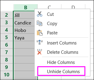
- Select the columns to the left and right of the column you want to unhide. For example, to show hidden column B, select columns A and C.
- Go to the Home tab > Cells group, and click Format > Hide & Unhide > Unhide columns.
How do I show all columns in Excel?
How to unhide columns in Excel:
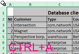
- Click on the small green triangle in the top left corner of your spreadsheet. This will select the entire spreadsheet.
- Now right-click anywhere in the entire selection and choose the Unhide option from the menu.
- You should now be able to see all of your columns.
Can’t see columns in Excel?
Individual Columns
- Open your Excel spreadsheet.
- Select both columns on either side of the hidden column.
- Click “Format” in the Cells group of the Home tab.
- Select “Visibility” followed by “Hide & Unhide” and “Unhide Columns” to make the missing column visible.
- Repeat for the other missing columns in the spreadsheet.
How do I unhide columns in Excel?
Unhide columns
- Select the adjacent columns for the hidden columns.
- Right-click the selected columns, and then select Unhide.
How do I unhide columns in sheets?
To unhide it on desktop or mobile, just click or tap the small arrow on either side of the hidden column or row. If you’re on a desktop, another way to unhide is to select a range of column on either side of the hidden column, right-click, and choose “Unhide Columns.”
Can’t see column headers in Excel?
Show or hide the Header Row
- Click anywhere in the table.
- Go to the Table tab on the Ribbon.
- In the Table Style Options group, select the Header Row check box to hide or display the table headers.
What is the shortcut key to unhide columns in Excel?
There are several dedicated keyboard shortcuts to hide and unhide rows and columns.
- Ctrl+9 to Hide Rows.
- Ctrl+0 (zero) to Hide Columns.
- Ctrl+Shift+( to Unhide Rows.
- Ctrl+Shift+) to Unhide Columns – If this doesn’t work for you try Alt,O,C,U (old Excel 2003 shortcut that still works).
Why did my Cells disappear in Excel?
Click on the View tab, then check the box for Gridlines in the Show group. If the background color for a cell is white instead of no fill, then it will appear that the gridlines are missing. Select the cells that are missing the gridlines, or hit Control + A to select the entire worksheet.
How do you show all Cells in Excel?
Display all contents with Wrap Text function
In Excel, the Wrap Text function will keep the column width and adjust the row height to display all contents in each cell. Select the cells that you want to display all contents, and click Home > Wrap Text. Then the selected cells will be expanded to show all contents.
How do I unhide all columns and rows in Excel?
To unhide all rows and columns, select the whole sheet as explained above, and then press Ctrl + Shift + 9 to show hidden rows and Ctrl + Shift + 0 to show hidden columns.
How do I unhide columns in Excel without a mouse?
Unhide Columns Using a Keyboard Shortcut
Press and hold down the Ctrl and the Shift keys on the keyboard. Press and release the 0 key without releasing the Ctrl and Shift keys.
Locate hidden cells
- Select the worksheet containing the hidden rows and columns that you need to locate, then access the Special feature with one of the following ways: Press F5 > Special. Press Ctrl+G > Special.
- Under Select, click Visible cells only, and then click OK.
How do I see column names in Excel?
Click the “Show row and column headers” check box so there is NO check mark in the box. Click “OK” to accept the change and close the “Excel Options” dialog box. The row and column headers are hidden from view on the selected worksheet. If you activate another worksheet, the row and column headers display again.
How do I unhide columns in Excel Mobile?
To unhide a hidden column or row
- Tap the column heading to the left of the hidden column, then drag the right selection handle to the right to select the next visible column. Or.
- On the shortcut bar, tap Unhide.
How do I unfreeze columns in Google Sheets?
Freeze or unfreeze rows or columns
- On your computer, open a spreadsheet in Google Sheets.
- Select a row or column you want to freeze or unfreeze.
- At the top, click View. Freeze.
- Select how many rows or columns to freeze.
How do you unlock columns in Google Sheets?
Unlock a Column or Row
- Right-click the column header and select Unlock Column (or click the lock icon under the column header).
- In the message that appears requesting your confirmation to unlock it, click OK.
What is Ctrl 0 Excel?
In Microsoft Excel and all other spreadsheet programs, pressing Ctrl+0 hides the column containing the active cell.
How do I unhide just one column in Excel?
Unhiding a Single Column
- Unhide the entire range and then rehide C:E and G:M.
- Enter cell F1 into the Name box and then use the controls available through the Format tool on the Home tab of the ribbon to unhide the column.
- Enter cell F1 into the Name box and then press Ctrl+Shift+0 to unhide the column.
What does Ctrl D do?
All major Internet browsers (e.g., Chrome, Edge, Firefox, Opera) pressing Ctrl + D creates a new bookmark or favorite for the current page. For example, you could press Ctrl + D now to bookmark this page.
How do I unhide columns in Excel 2016?
Select the Home tab from the toolbar at the top of the screen. Select Cells > Format > Hide & Unhide > Unhide Columns. Now column A should be unhidden in your Excel spreadsheet.
How do I unhide columns in Excel for Mac?
How to unhide columns in Excel
- Open Microsoft Excel on your PC or Mac computer.
- Highlight the column on either side of the column you wish to unhide in your document.
- Right-click anywhere within a selected column.
- Click “Unhide” from the menu.
- You can also manually click or drag to expand a hidden column.
Источник
Unhide the first column or row in a worksheet
If the first row (row 1) or column (column A) is not displayed in the worksheet, it is a little tricky to unhide it because there is no easy way to select that row or column. You can select the entire worksheet, and then unhide rows or columns ( Home tab, Cells group, Format button, Hide & Unhide command), but that displays all hidden rows and columns in your worksheet, which you may not want to do. Instead, you can use the Name box or the Go To command to select the first row and column.
To select the first hidden row or column on the worksheet, do one of the following:
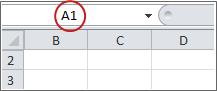
In the Name Box next to the formula bar, type A1, and then press ENTER.
On the Home tab, in the Editing group, click Find & Select, and then click Go To. In the Reference box, type A1, and then click OK.
On the Home tab, in the Cells group, click Format.
Do one of the following:
Under Visibility, click Hide & Unhide, and then click Unhide Rows or Unhide Columns.
Under Cell Size, click Row Height or Column Width, and then in the Row Height or Column Width box, type the value that you want to use for the row height or column width.
Tip: The default height for rows is 15, and the default width for columns is 8.43.
If you don’t see the first column (column A) or row (row 1) in your worksheet, it might be hidden. Here’s how to unhide it. In this picture column A and row 1 are hidden.
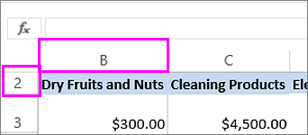
To unhide column A, right-click the column B header or label and pick Unhide Columns.
To unhide row 1, right-click the row 2 header or label and pick Unhide Rows.
Tip: If you don’t see Unhide Columns or Unhide Rows, make sure you’re right-clicking inside the column or row label.
Источник
How to Quickly Unhide COLUMNS in Excel (A Simple Guide)
Watch Video – How to Unhide Columns in Excel
If you prefer written instruction instead, below is the tutorial.
Hidden rows and columns can be quite irritating at times.
Especially if someone else has hidden these and you forget to unhide it (or even worse, you don’t know how to unhide these).
While I can’t do anything about the first issue, I can show you how to unhide columns in Excel (the same techniques can also be used to unhide rows).
It may happen that one of the methods of unhiding columns/rows may not work for you. In that case, it is good to know the alternatives that can work.
This Tutorial Covers:
How to Unhide Columns in Excel
There are many different situations where you may need to unhide the columns:
- Multiple columns are hidden and you want to unhide all columns at once
- You want to unhide a specific column (in between two columns)
- You want to unhide the first column
Let’s go through each for these scenarios and see how to unhide the columns.
Unhide All Columns At One Go
If you have a worksheet that has multiple hidden columns, you don’t need to go hunt each one and bring it to light.
You can do that all in one go.
And there are multiple ways to do this.
Using the Format Option
Here are the steps to unhide all columns at one go:
- Click on the small triangle at the top left of the worksheet area. This will select all the cells in the worksheet.
- Right-click anywhere in the worksheet area.
- Click on Unhide.
No matter where that pesky column is hidden, this will unhide it.
Using VBA
If you need to do this often, you can also use VBA to get this done.
The below code will unhide column in the worksheet.
You need to place this code in the VB Editor (in a module).
If you want to learn how to do this with VBA, read a detailed guide on how to run a macro in Excel.
Using a Keyboard Shortcut
If you’re more comfortable using keyboard shortcuts, there is a way to unhide all columns with a few keystrokes.
Here are the steps:
- Select any cell in the worksheet.
- Press Control-A-A (hold the control key and press A twice). This will select all the cells in the worksheet
- Use the following shortcut – ALT H O U L (one key at a time)
If you can get hang of this keyboard shortcut, it could be a lot faster to unhide columns.
Note: The reason you need to press A twice when holding the control key is that sometimes when you press Control A, it only selects the used range in Excel (or the area that has the data) and you need to press the A again to select the entire worksheet.
Another keyword shortcut that works for some and not for others is Control 0 (from a numeric keypad) or Control Shift 0 from a non-numeric keypad. It used to work for me earlier but doesn’t work anymore. Here is some discussion on why it may happen. I suggest you use the longer (ALT HOUL) shortcut that works every time.
Unhide Columns in Between Selected Columns
There are multiple ways you can quickly unhide columns in between selected columns. The methods shown here are useful when you want to unhide a specific column(s).
Let’s go through these one-by-one (and you can choose to use that you find the best).
Using a Keyboard Shortcut
Below are the steps:
- Select the columns that contain the hidden columns in between. For example, if you are trying to unhide column C, then select column B and D.

- Use the following shortcut – ALT H O U L (one key at a time)

This will instantly unhide the columns.
Using the Mouse
One quick and easy way to unhide a column is to use the mouse.
Below are the steps:
- Hover your mouse in between the columns alphabets that have the hidden column(s). For example, if Column C is hidden, then hover the mouse between Column B and D (at the top of the worksheet). You will see a double line icon with arrows pointing on left and right.
- Hold the left key of the mouse and drag it to the right. It will make the hidden column appear.

Using the Format Option in the Ribbon
Under the home tab in the ribbon, there are options to hide and unhide columns in Excel.
Here is how to use it:
Another way of accessing this option is by selecting the columns and right clicking using the mouse. In the menu that appears, select the unhide option.

Using VBA
Below is the code that you can use to unhide columns in between the selected columns.
Sub UnhideAllColumns()
Selection.EntireColumn.Hidden = False
End Sub
You need to place this code in the VB Editor (in a module).
If you want to learn how to do this with VBA, read a detailed guide on how to run a macro in Excel.
By Changing the Column Width
There is a possibility that none of these methods work when you try to unhide column in Excel. It happens when you change the Column Width to 0. In that case, even if you unhide the column, it’s width still remains 0, and hence you can’t see it or select it.
Below are the steps to change the column width:
This is by far the most reliable way to unhide columns in Excel. If everything fails, just change the column width.
Unhide the First Column
Unhiding the first column can be a little bit tricky.
You can use many of the methods covered above, with a little bit of extra work.
Let me show you a few ways.
Use the Mouse to Drag the First Column
Even when the first column is hidden, Excel allows you to select it and drag it to make it visible.
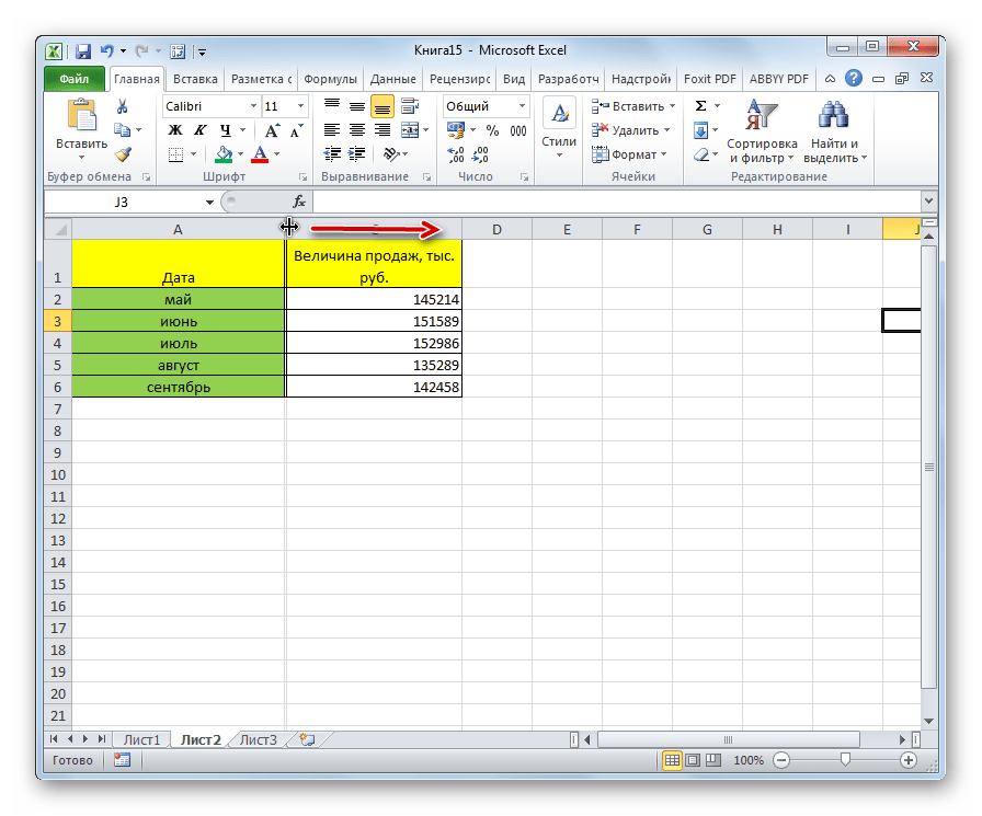
To do this, hover the cursor on the left edge of column B (or whatever is the leftmost visible column).
The cursor would change into a double arrow pointer as shown below.

Hold the left mouse button and drag the cursor to the right. You will see that it unhides the hidden column.

Go to a Cell in the First Column and Unhide it
But how do you go to any cell in the column that’s hidden?
You use the Name Box (it’s left to the formula bar).

Enter A1 in the Name Box. It will instantly take you to the A1 cell. Since the first column is hidden, you won’t be able to see it, but be assured that it’s selected (you’ll still see a thin line just left of B1).
Once the hidden column cell is selected, follow the below steps:
- Click the Home tab.
- In the Cells group, click on Format.
- Hover the cursor on the ‘Hide & Unhide’ option.
- Click on ‘Unhide Columns’
Select the First Column and Unhide it
Again! How do you select it when it’s hidden?
Well, there are many different ways to skin the cat.
And this is just another method in my kitty (this is the last cat sounding reference I promise).
When you select the leftmost visible cell and drag the cursor to the left (where there are row numbers), you end up selecting all the hidden columns (even when you don’t see it).

Once you have select all the hidden columns, follow the below steps:
- Click the Home tab.
- In the Cells group, click on Format.
- Hover the cursor on the ‘Hide & Unhide’ option.
- Click on ‘Unhide Columns’
Excel has an ‘Inspect Document’ feature that is meant to quickly scan the workbook and give you some details about it.
And one of the things that you can do that ‘Inspect Document’ is to quickly check how many hidden columns or hidden rows are there in the workbook.
This might be useful when you get the workbook from someone and want to quickly inspect it.
Below are the steps on how to check the total number of hidden columns or hidden rows:
- Open the workbook
- Click on the File tab
- In the Info options, click on the ‘Check for Issues’ button (it’s next to the Inspect Workbook text).
- Click on Inspect Document.
- In the Document Inspector, make sure Hidden Rows and Columns option is checked.
- Click the Inspect button.


This will show you the total number of hidden rows and columns.

It also gives you the option to delete all these hidden rows/columns. This can be the case if there is extra data that has been hidden and is not needed. Instead of finding hidden rows and columns, you can quickly delete these from this option.
You May Also Like the following Excel Tips/Tutorials:
Источник
Hide or show rows or columns
Hide or unhide columns in your spreadsheet to show just the data that you need to see or print.

Hide columns
-
Select one or more columns, and then press Ctrl to select additional columns that aren’t adjacent.
-
Right-click the selected columns, and then select Hide.
Note: The double line between two columns is an indicator that you’ve hidden a column.
Unhide columns
-
Select the adjacent columns for the hidden columns.
-
Right-click the selected columns, and then select Unhide.
Or double-click the double line between the two columns where hidden columns exist.
Need more help?
You can always ask an expert in the Excel Tech Community or get support in the Answers community.
See Also
Unhide the first column or row in a worksheet
Need more help?
Working in Excel, sometimes there is a need to hide part of displayed data.
The most handy way — is to hide individual columns or rows. For example, during the presentation or before preparing document to print.
How to hide columns and rows in Excel?
Let’s say you have the table in what you need to display only the most significant data for better reading of performance. In order to do this, we will do the following:
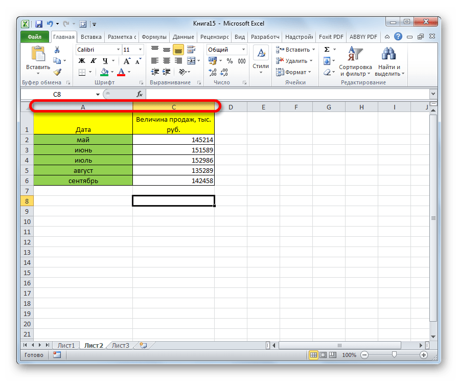
- Select the column data of what you need to hide – for instance, the column C.
- On a selected column to right-click of mouse and select the option «Hide» CTRL+0 (for columns) CTRL+9 (for rows).
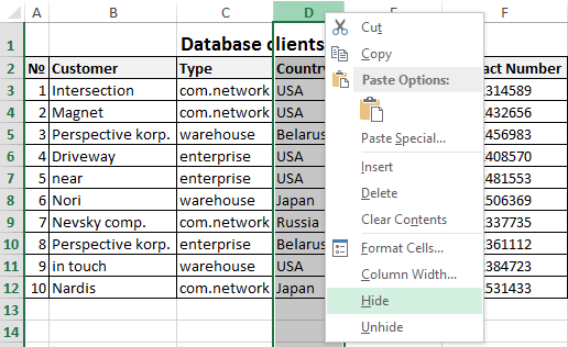
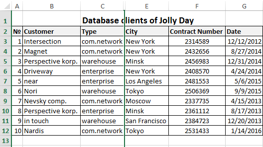
The column was hidden, but not deleted. This is evidenced by the priority of the alphabet`s letters in the names of columns (A; B; D; E).
Remark. If you want to hide multiple columns, highlight them before hiding. You can selectively highlight multiple columns with CTRL key pressed. In a similar way, you can hide the rows.
How to display hidden columns and rows in Excel?
To redisplay to the hidden column, you must select 2 of its contiguous (contiguous) columns. Then to generate the context menu, right-click and choose the option «Unhide».
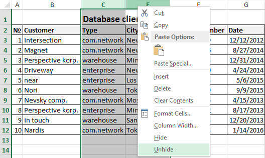
The similar actions are performed in order to open the hidden rows in Excel.
If the sheet is hidden many rows and columns and you want to display all at once, you must highlight the whole worksheet by pressing CTRL+A. Further a separate call to the context menu for the columns to choose the option «Show» and then for the rows, or in reverse order (for rows then for columns).
To select the entire sheet you can by clicking in the intersection of column headings and rows.
About these and other methods to select of an entire sheet and bands you have already known from the previous lessons.
Содержание
- Показ скрытых столбцов
- Способ 1: ручное перемещение границ
- Способ 2: контекстное меню
- Способ 3: кнопка на ленте
- Вопросы и ответы

При работе в Excel иногда требуется скрыть столбцы. После этого, указанные элементы перестают отображаться на листе. Но, что делать, когда снова нужно включить их показ? Давайте разберемся в этом вопросе.
Показ скрытых столбцов
Прежде, чем включить отображение скрытых столбов, нужно разобраться, где они располагаются. Сделать это довольно просто. Все столбцы в Экселе помечены буквами латинского алфавита, расположенными по порядку. В том месте, где этот порядок нарушен, что выражается в отсутствии буквы, и располагается скрытый элемент.
Конкретные способы возобновления отображения скрытых ячеек зависят от того, какой именно вариант применялся для того, чтобы их спрятать.
Способ 1: ручное перемещение границ
Если вы скрыли ячейки путем перемещения границ, то можно попытаться показать строку, переместив их на прежнее место. Для этого нужно стать на границу и дождаться появления характерной двусторонней стрелки. Затем нажать левую кнопку мыши и потянуть стрелку в сторону.
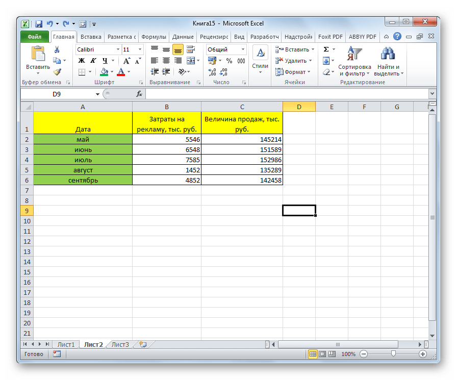
После выполнения данной процедуры ячейки будут отображаться в развернутом виде, как это было прежде.
Правда, нужно учесть, что если при скрытии границы были подвинуты очень плотно, то «зацепиться» за них таким способом будет довольно трудно, а то и невозможно. Поэтому, многие пользователи предпочитают решить этот вопрос, применяя другие варианты действий.
Способ 2: контекстное меню
Способ включения отображения скрытых элементов через контекстное меню является универсальным и подойдет во всех случаях, без разницы с помощью какого варианта они были спрятаны.
- Выделяем на горизонтальной панели координат соседние секторы с буквами, между которыми располагается скрытый столбец.
- Кликаем правой кнопкой мыши по выделенным элементам. В контекстном меню выбираем пункт «Показать».
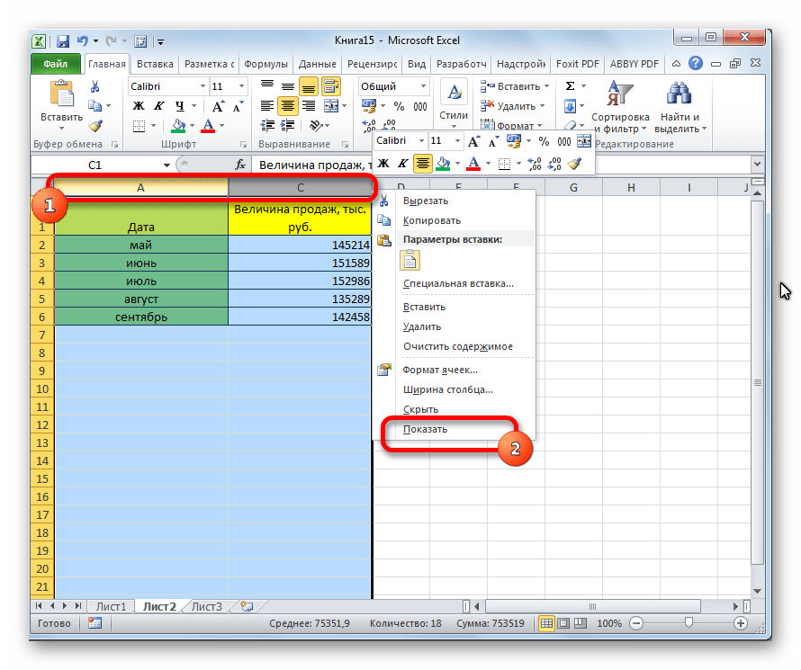
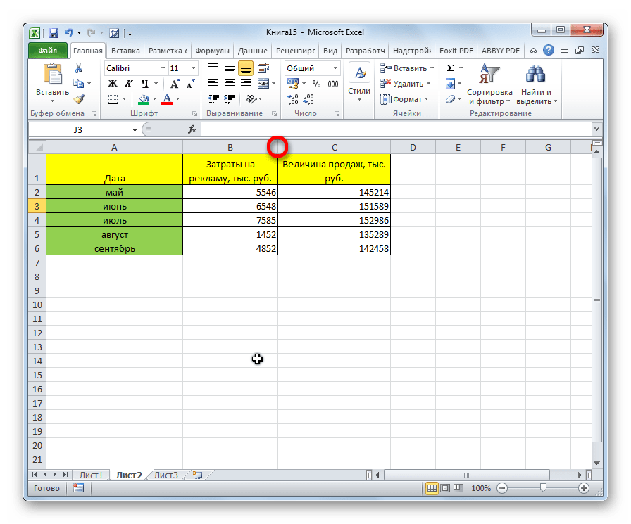
Теперь спрятанные столбцы начнут отображаться снова.
Способ 3: кнопка на ленте
Использование кнопки «Формат» на ленте, как и предыдущий вариант, подойдет для всех случаев решения поставленной задачи.

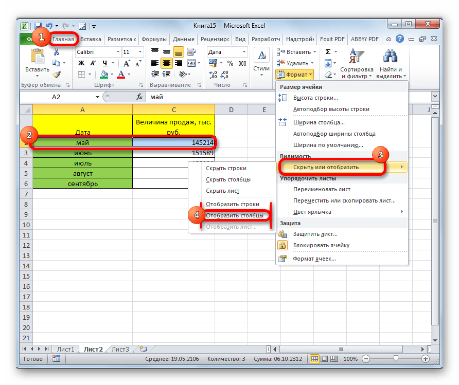
- Перемещаемся во вкладку «Главная», если находимся в другой вкладке. Выделяем любые соседние ячейки, между которыми находится скрытый элемент. На ленте в блоке инструментов «Ячейки» кликаем по кнопке «Формат». Открывается меню. В блоке инструментов «Видимость» перемещаемся в пункт «Скрыть или отобразить». В появившемся списке выбираем запись «Отобразить столбцы».
- После этих действий соответствующие элементы опять станут видимыми.
Урок: Как скрыть столбцы в Excel
Как видим, существует сразу несколько способов включить отображение скрытых столбцов. При этом, нужно заметить, что первый вариант с ручным перемещением границ подойдет только в том случае, если ячейки были спрятаны таким же образом, к тому же их границы не были сдвинуты слишком плотно. Хотя, именно этот способ и является наиболее очевидным для неподготовленного пользователя. А вот два остальных варианта с использованием контекстного меню и кнопки на ленте подойдут для решения данной задачи в практически любой ситуации, то есть, они являются универсальными.
Еще статьи по данной теме:
Помогла ли Вам статья?
![]()
Загрузить PDF
![]()
Загрузить PDF
Из данной статьи вы узнаете, как отображать скрытые столбцы в Microsoft Excel. Это можно сделать в Windows и в Mac OS X.
Шаги
-
1
Откройте таблицу Excel. Для этого дважды щелкните по файлу Excel или дважды щелкните по значку программы Excel, а затем выберите имя файла на главной странице. Так вы откроете таблицу со скрытыми столбцами в Excel.
-
2
Выделите столбцы с обеих сторон от скрытого столбца. Зажмите клавишу ⇧ Shift, а затем щелкните по букве над столбцом слева от скрытого столбца и по букве над столбцом справа от скрытого столбца. Столбцы будут выделены.
- Например, если скрыть столбец B, зажмите ⇧ Shift и щелкните по A и C.
- Если нужно отобразить столбец A, введите «A1» (без кавычек) в поле «Имя», которое расположено слева от строки формул.
-
3
Перейдите на вкладку Главная. Она находится в верхней левой части окна Excel. Так вы откроете панель инструментов «Главная».
-
4
Нажмите Формат. Эта кнопка находится в разделе «Ячейки» вкладки «Главная»; этот раздел расположен в правой части панели инструментов. Откроется выпадающее меню.[1]
-
5
Выберите Скрыть или отобразить. Эта опция находится в разделе «Видимость» выпадающего меню «Формат». Откроется всплывающее меню.
-
6
Нажмите Отобразить столбцы. Эта опция находится в нижней части меню «Скрыть или отобразить». Скрытый столбец будет отображен (между двумя выделенными столбцами).
Реклама


Советы
- Если некоторые столбцы не отобразились, возможно, значение их ширины равно 0 или другой малой величине. Чтобы расширить столбец, поместите курсор на правую границу столбца и перетащите ее.
- Чтобы отобразить все скрытые столбцы, нажмите кнопку «Выбрать все», значок которой представляет собой пустой прямоугольник слева от столбца «A» и над строкой «1». Затем выполните действия, описанные в этой статье.
Реклама
Об этой статье
Эту страницу просматривали 61 685 раз.