Use the DATEDIF function when you want to calculate the difference between two dates. First put a start date in a cell, and an end date in another. Then type a formula like one of the following.
Warning: If the Start_date is greater than the End_date, the result will be #NUM!.
Difference in days
In this example, the start date is in cell D9, and the end date is in E9. The formula is in F9. The “d” returns the number of full days between the two dates.
Difference in weeks
In this example, the start date is in cell D13, and the end date is in E13. The “d” returns the number of days. But notice the /7 at the end. That divides the number of days by 7, since there are 7 days in a week. Note that this result also needs to be formatted as a number. Press CTRL + 1. Then click Number > Decimal places: 2.
Difference in months
In this example, the start date is in cell D5, and the end date is in E5. In the formula, the “m” returns the number of full months between the two days.
Difference in years
In this example, the start date is in cell D2, and the end date is in E2. The “y” returns the number of full years between the two days.
Calculate age in accumulated years, months, and days
You can also calculate age or someone’s time of service. The result can be something like “2 years, 4 months, 5 days.”
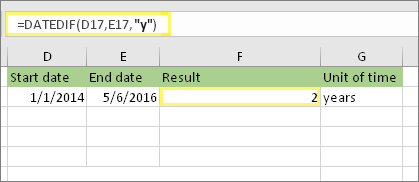
1. Use DATEDIF to find the total years.
In this example, the start date is in cell D17, and the end date is in E17. In the formula, the “y” returns the number of full years between the two days.
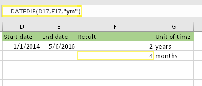
2. Use DATEDIF again with “ym” to find months.
In another cell, use the DATEDIF formula with the “ym” parameter. The “ym” returns the number of remaining months past the last full year.
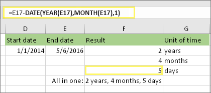
3. Use a different formula to find days.
Now we need to find the number of remaining days. We’ll do this by writing a different kind of formula, shown above. This formula subtracts the first day of the ending month (5/1/2016) from the original end date in cell E17 (5/6/2016). Here’s how it does this: First the DATE function creates the date, 5/1/2016. It creates it using the year in cell E17, and the month in cell E17. Then the 1 represents the first day of that month. The result for the DATE function is 5/1/2016. Then, we subtract that from the original end date in cell E17, which is 5/6/2016. 5/6/2016 minus 5/1/2016 is 5 days.
Warning: We don’t recommend using the DATEDIF «md» argument because it may calculate inaccurate results.
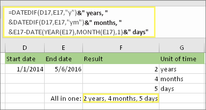
4. Optional: Combine three formulas in one.
You can put all three calculations in one cell like this example. Use ampersands, quotes, and text. It’s a longer formula to type, but at least it’s all in one. Tip: Press ALT+ENTER to put line breaks in your formula. This makes it easier to read. Also, press CTRL+SHIFT+U if you can’t see the whole formula.
Download our examples
Other date and time calculations
As you saw above, the DATEDIF function calculates the difference between a start date and an end date. However, instead of typing specific dates, you can also use the TODAY() function inside the formula. When you use the TODAY() function, Excel uses your computer’s current date for the date. Keep in mind this will change when the file is opened again on a future day.
Please note that at the time of this writing, the day was October 6, 2016.
Use the NETWORKDAYS.INTL function when you want to calculate the number of workdays between two dates. You can also have it exclude weekends and holidays too.
Before you begin: Decide if you want to exclude holiday dates. If you do, type a list of holiday dates in a separate area or sheet. Put each holiday date in its own cell. Then select those cells, select Formulas > Define Name. Name the range MyHolidays, and click OK. Then create the formula using the steps below.
1. Type a start date and an end date.
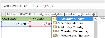
In this example, the start date is in cell D53 and the end date is in cell E53.
2. In another cell, type a formula like this:
Type a formula like the above example. The 1 in the formula establishes Saturdays and Sundays as weekend days, and excludes them from the total.
Note: Excel 2007 doesn’t have the NETWORKDAYS.INTL function. However, it does have NETWORKDAYS. The above example would be like this in Excel 2007: =NETWORKDAYS(D53,E53). You don’t specify the 1 because NETWORKDAYS assumes the weekend is on Saturday and Sunday.
3. If necessary, change the 1.
If Saturday and Sunday are not your weekend days, then change the 1 to another number from the IntelliSense list. For example, 2 establishes Sundays and Mondays as weekend days.
If you are using Excel 2007, skip this step. Excel 2007’s NETWORKDAYS function always assumes the weekend is on Saturday and Sunday.
4. Type the holiday range name.
If you created a holiday range name in the “Before you begin” section above, then type it at the end like this. If you don’t have holidays, you can leave the comma and MyHolidays out. If you are using Excel 2007, the above example would be this instead: =NETWORKDAYS(D53,E53,MyHolidays).
Tip: If you don’t want to reference a holiday range name, you can also type a range instead, like D35:E:39. Or, you could type each holiday inside the formula. For example if your holidays were on January 1 and 2 of 2016, you’d type them like this: =NETWORKDAYS.INTL(D53,E53,1,{«1/1/2016″,»1/2/2016»}). In Excel 2007, it would look like this: =NETWORKDAYS(D53,E53,{«1/1/2016″,»1/2/2016»})
You can calculate elapsed time by subtracting one time from another. First put a start time in a cell, and an end time in another. Make sure to type a full time, including the hour, minutes, and a space before the AM or PM. Here’s how:
1. Type a start time and end time.
In this example, the start time is in cell D80 and the end time is in E80. Make sure to type the hour, minute, and a space before the AM or PM.
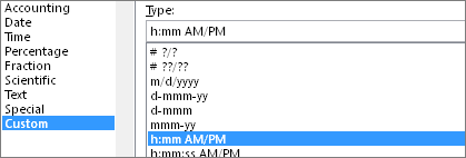
2. Set the h:mm AM/PM format.
Select both dates and press CTRL + 1 (or 
3. Subtract the two times.
In another cell, subtract the start time cell from the end time cell.
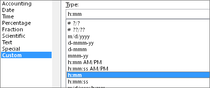
4. Set the h:mm format.
Press CTRL + 1 (or 
To calculate the time between two dates and times, you can simply subtract one from the other. However, you must apply formatting to each cell to ensure that Excel returns the result you want.
1. Type two full dates and times.
In one cell, type a full start date/time. And in another cell, type a full end date/time. Each cell should have a month, day, year, hour, minute, and a space before the AM or PM.
2. Set the 3/14/12 1:30 PM format.
Select both cells, and then press CTRL + 1 (or 
3. Subtract the two.
In another cell, subtract the start date/time from the end date/time. The result will probably look like a number and decimal. You’ll fix that in the next step.
4. Set the [h]:mm format.
Press CTRL + 1 (or 
Related Topics
DATEDIF function
NETWORKDAYS.INTL function
NETWORKDAYS
More date and time functions
Calculate the difference between two times
17 авг. 2022 г.
читать 1 мин
Мы можем использовать функцию DATEDIF() для вычисления разницы между двумя датами в Excel.
Эта функция использует следующий синтаксис:
=DATEDIF(Начальная_Дата, Конечная_Дата, Метрика)
куда:
- Start_Date: дата начала
- End_Date: Дата окончания
- Метрика: метрика для расчета. Варианты включают:
- «д»: дни
- «м»: Месяцы
- «г»: годы
Важно отметить, что эта функция не появится автоматически в Excel, пока вы полностью не введете =РАЗНДАТ( в одну из ячеек.
В следующих примерах показано, как использовать эту функцию для вычисления разницы между двумя датами в Excel.
Пример 1: разница в днях
На следующем изображении показано, как рассчитать разницу (в днях) между двумя датами:
Это говорит нам о том, что между 01.01.2018 и 01.02.2021 1127 полных дней.
Пример 2: разница в месяцах
На следующем изображении показано, как рассчитать разницу (в месяцах) между двумя датами:
Пример 3: Разница в годах
На следующем изображении показано, как рассчитать разницу (в годах) между двумя датами:
Пример 4: Разница в годах и месяцах
На следующем рисунке показано, как рассчитать разницу (в годах и месяцах) между двумя датами:
Вы можете найти больше руководств по Excel на этой странице .
Написано

Замечательно! Вы успешно подписались.
Добро пожаловать обратно! Вы успешно вошли
Вы успешно подписались на кодкамп.
Срок действия вашей ссылки истек.
Ура! Проверьте свою электронную почту на наличие волшебной ссылки для входа.
Успех! Ваша платежная информация обновлена.
Ваша платежная информация не была обновлена.
We can use the DATEDIF() function to calculate the difference between two dates in Excel.
This function uses the following syntax:
=DATEDIF(Start_Date, End_Date, Metric)
where:
- Start_Date: The start date
- End_Date: The end date
- Metric: The metric to calculate. Options include:
- “d”: Days
- “m”: Months
- “y”: Years
It’s important to note that this function won’t automatically appear in Excel until you completely type =DATEDIF( into one of the cells.
The following examples show how to use this function to calculate the difference between two dates in Excel.
Example 1: Difference in Days
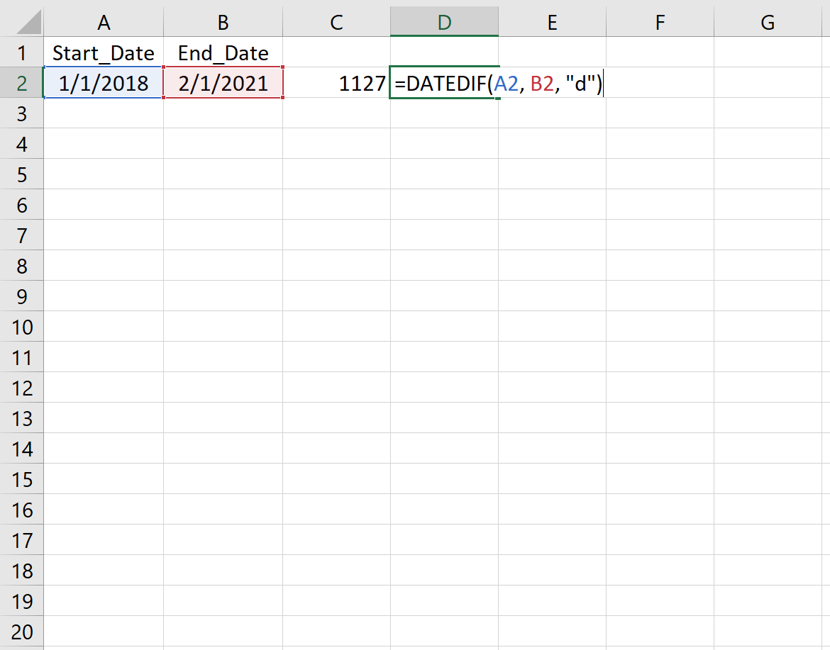
The following image shows how to calculate the difference (in days) between two dates:
This tells us that there are 1,127 full days between 1/1/2018 and 2/1/2021.
Example 2: Difference in Months
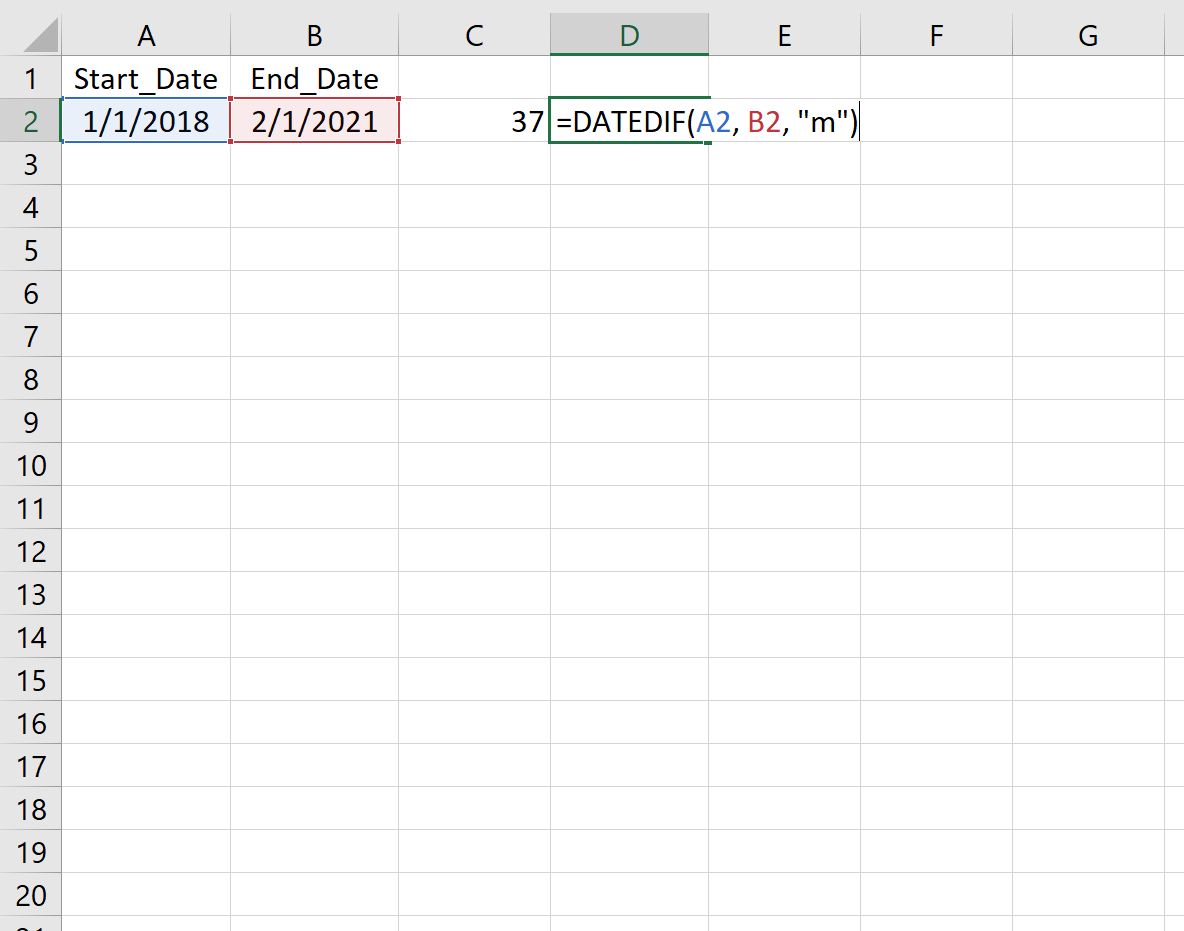
The following image shows how to calculate the difference (in months) between two dates:
Example 3: Difference in Years
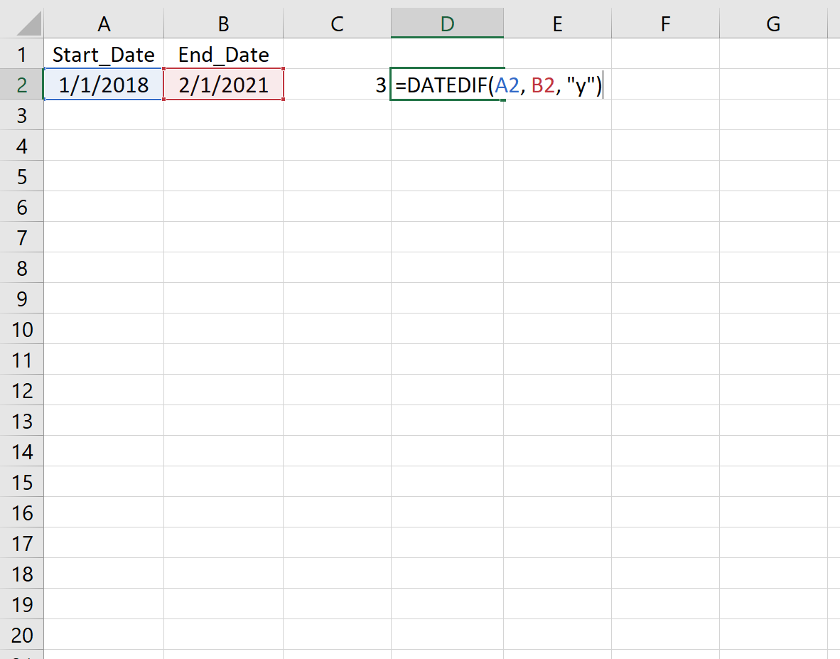
The following image shows how to calculate the difference (in years) between two dates:
Example 4: Difference in Years & Months
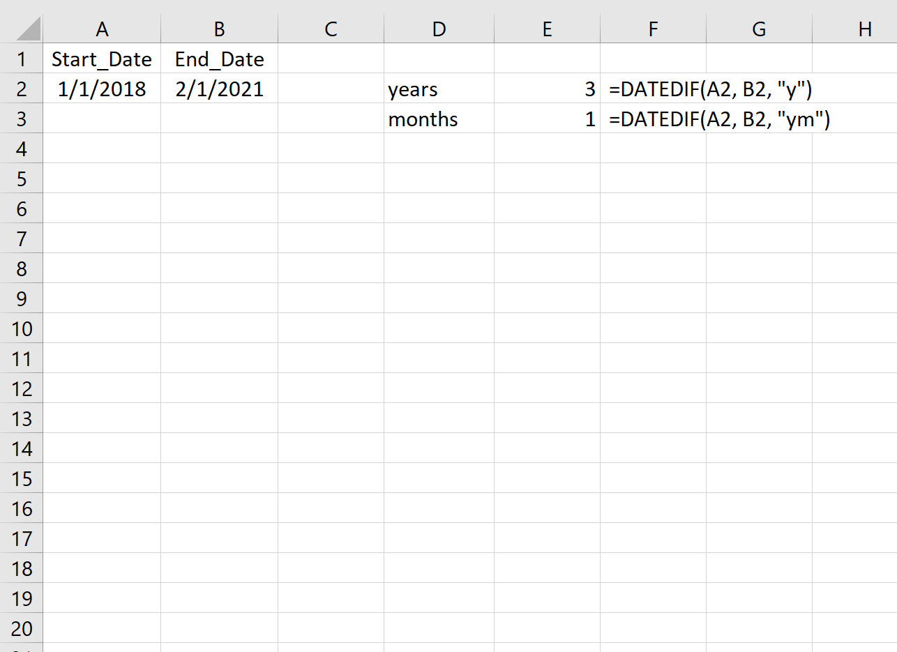
The following image shows how to calculate the difference (in years and months) between two dates:
You can find more Excel tutorials on this page.
The DATEDIF (Date + Dif) function is a «compatibility» function that comes from Lotus 1-2-3. For a long time, official documentation on DATEDIF was sparse. Even now (May 2021), Excel will not help you fill in arguments for DATEDIF like other functions. As the late Chip Pearson once wrote in his immortal words: DATEDIF is treated as the drunk cousin of the Formula family. Excel knows it lives a happy and useful life, but will not speak of it in polite conversation. Yet DATEDIF remains a very useful function for certain problems.
Time units
The DATEDIF function can calculate the time between a start_date and an end_date in years, months, or days. The time unit is specified with the unit argument, which is supplied as text. The table below summarizes available unit values and the result for each. Time units can be given in upper or lower case (i.e. «ym» is equivalent to «YM»).
| Unit | Result |
|---|---|
| «y» | Difference in complete years |
| «m» | Difference in complete months |
| «d» | Difference in days |
| «md» | Difference in days, ignoring months and years |
| «ym» | Difference in months, ignoring years |
| «yd» | Difference in days, ignoring years |
Example 1 — Basic usage
In the example shown above, column B contains the date January 1, 2016 and column C contains the date March 1, 2018. In column E:
E5=DATEDIF(B5,C5,"y") // returns 2
E6=DATEDIF(B6,C6,"m") // returns 26
E7=DATEDIF(B7,C7,"d")// returns 790
Example 2 — Difference in days
The DATEDIF function can calculate the difference between dates in days in three different ways: (1) total days, (2) days ignoring years, and (3) days ignoring months and years. The screenshot below shows all three methods, with a start date of June 15, 2015, and an end date of September 15, 2021:
The formulas used for these calculations are as follows:
=DATEDIF(B5,C5,"d") // total days
=DATEDIF(B6,C6,"yd") // days ignoring years
=DATEDIF(B7,C7,"md") // days ignoring months and years
Note that because Excel dates are just large serial numbers, the first formula does not need DATEDIF and could be written as simply the end date minus the start date:
=C5-B5 // end-start = total days
Example 3 — Difference in months
The DATEDIF function can calculate the difference between dates in months in two different ways: (1) total complete months, (2) complete months ignoring years. The screenshot below shows both methods, with a start date of June 15, 2015, and an end date of September 15, 2021:
=DATEDIF(B5,C5,"m") // complete months
=DATEDIF(B6,C6,"ym") // complete months ignoring years
DATEDIF always rounds months down to the last complete number of months. This means DATEDIF rounds the result down even when it is very close to the next whole month. In addition, DATEDIF may not work as expected when start and end dates are «end of month» dates. This example provides more information and alternatives.
Example 4 — Difference in years
The DATEDIF function can calculate the difference between dates in complete years with just one method, shown below:
=DATEDIF(B5,C5,"y") // complete years
=DATEDIF(B6,C6,"y") // complete years
=YEARFRAC(B7,C7) // fractional  years with YEARFRAC
Notice in row 6 the difference is almost 6 years, but not quite. Because DATEDIF only calculates complete years, the result is still 5. In row 7 we use the YEARFRAC function to calculate a more accurate result.
Example 5 — Age from birthday
The DATEDIF function can be used together with the TODAY function to calculate current age from a birth date. With a full birth date in A1, the formula is:
=DATEDIF(A1,TODAY(),"y")
Read a complete explanation here.
Notes
- Excel will not help you fill in the DATEDIF function like other functions.
- DATEDIF will throw a #NUM error if start_date is greater than the end_date. If you are working with a more complex formula where start dates and end dates may be unknown, or out of bounds, you can trap the error with the IFERROR function, or use MIN and MAX to sort out dates.
- Microsoft recommends not using the «MD» value for unit because it «may result in a negative number, a zero, or an inaccurate result».
DATEDIF Function in Excel
The DATEDIF is a date function used to find the difference between two given dates. Now, these differences can be in years, months, or days. It takes two dates as an argument and one keyword to specify which type of difference is desired for the output. The output for this function is an integer, and the method to use this function is as follows =DATEDIF(start_date, end_date, unit). However, this function is compatible with Excel 2000 and previous versions of Excel.
For example, suppose we have 1/1/2013 as a start date in column A5 and 31/7/17 as an end date in column B5. We want to know the difference between the two days in column C. In this scenario, we can use the DATEDIF function in Excel. The formula we can use as:
=DATEDIF(A5, B5,”C”)
As a result, it will give us 1,672 days.
Table of contents
- DATEDIF Function in Excel
- Syntax
- Number of Units Available
- How to use the DATEDIF Function in Excel? (with Examples)
- Example #1 – Number of days between the two dates
- Example #2 – Count the number of days ignoring years
- Example #3 – Count the number of months between the two dates
- Example #4 – Find the days excluding years and months.
- Example #5 – Find the days excluding days and years.
- Example #6 – Find the years.
- Advantages
- Disadvantages
- Things to Remember
- Recommended Articles
- Syntax
Syntax
DATEDIF(start_date, end_date, unit)
- Start_date – the initial date of the period you want to calculate.
- Unit: The time unit to utilize while ascertaining the difference between two dates.
- End_date – the ending date of the period.
Number of Units Available
- #1 – Y (Years): Y is used in a formula to find the number of complete years between beginning and end dates.
- #2 – M (Months): used in a formula to find the number of entire months between the dates.
- #3 – D (Days): D is used in a formula to see the number of days between the beginning and end dates.
- #4 – MD (Days barring years and months): MD is used in a formula to find the date contrast in days, disregarding months and years.
- #5 – YD (Days barring years): YD is used in a formula to find the date contrast in days, disregarding years.
- #6 – YM (Months barring days and years): YM is used in a formula to find the date contrast in months, ignoring days and years.
How to use the DATEDIF Function in Excel? (with Examples)
You can download this DATEDIF Function Excel Template here – DATEDIF Function Excel Template
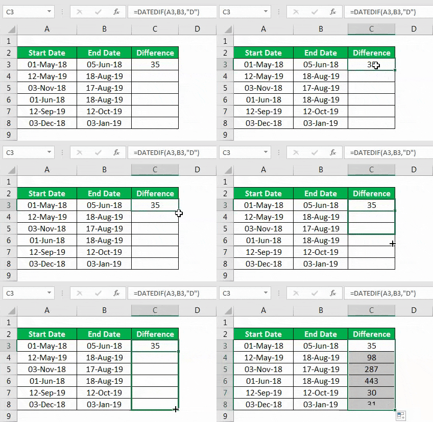
Example #1 – Number of days between the two dates
Follow the below steps to use the datedif function in Excel.
- We will use the following data to find the no. of days between 2 dates.
- Then, we will enter the DATEDIF formula in the first row and use “D” as a unit.
- Now, we should press the “Enter” key and find the difference in days between the two dates.
- If we drag the formula, we will get the result for all the dates. So please find the same in the figure shown below.
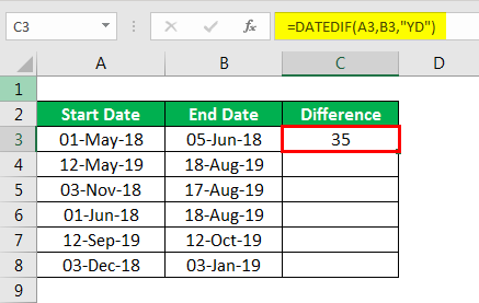
Example #2 – Count the number of days ignoring years
- Step 1: In this example, we will use the following data to find the no. of days, ignoring years.
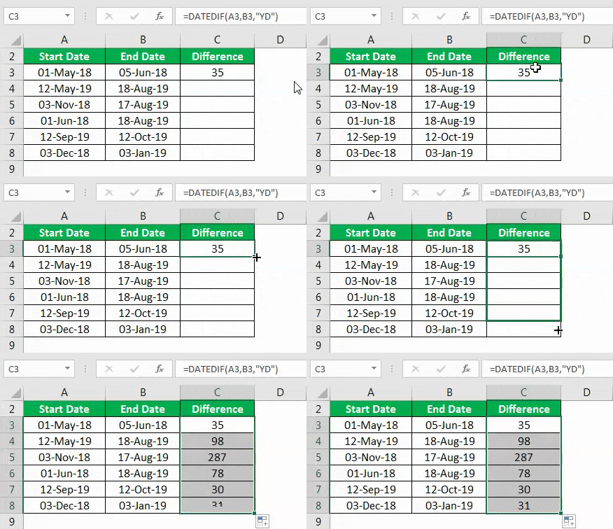
- Step 2: First, we must enter the DATEDIF formula in the first row and use “YD” as a unit in a formula.
- Step 3: Then, we need topress the “Enter” key, and we will find the difference in days between the two dates.
- Step 4: If we drag the formula, we will get the result for all the dates. Please find the same in the figure shown below.
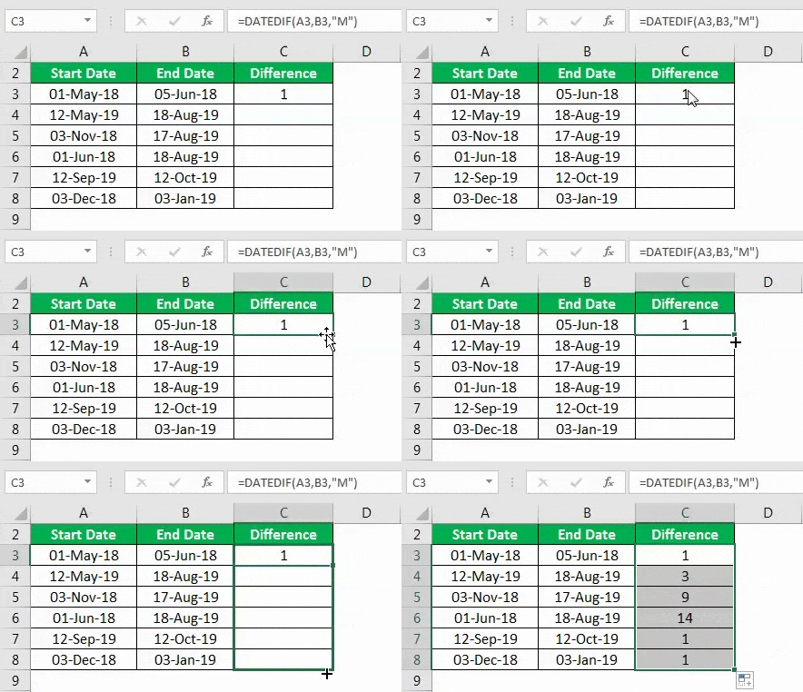
Example #3 – Count the number of months between the two dates
- Step 1: We will use the following data to find the number of months between the two dates.
- Step 2: Next, we will enter the DATEDIF formula in the first row and use “M” as a unit in a formula
- Step 3: Then, we should press the “Enter” key and find the difference in days between the two dates in excelThe date function in excel is a date and time function representing the number provided as arguments in a date and time code. The result displayed is in date format, but the arguments are supplied as integers.read more.
- Step 4: If we drag the formula, we will get the result for all the dates. Please find the same in the figure shown below.
Example #4 – Find the days excluding years and months.
- Step 1: We will use the following data to find the days, excluding years and months.
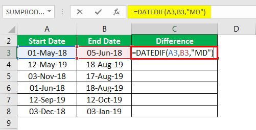
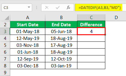
- Step 2: We must enter the DATEDIF formula in the first row, and use “MD” as a unit in a formula.
- Step 3: We will find the difference in days between the two dates. We will press the “Enter” key.
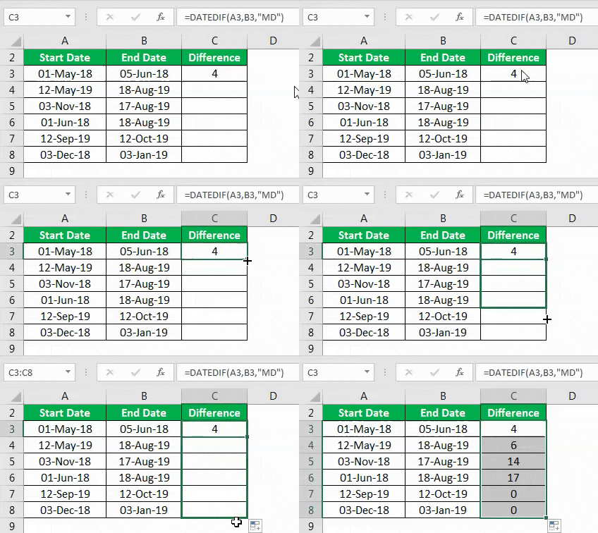
- Step 4: If we drag the formula, we will get the result for all the dates. Please find the same in the figure shown below.
Example #5 – Find the days excluding days and years.
- Step 1: We will use the following data to find the days, excluding days and years.
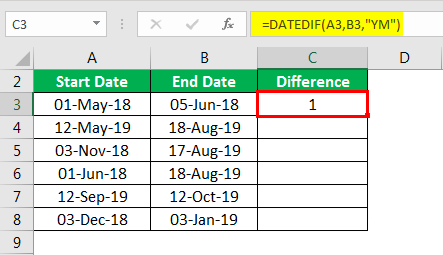
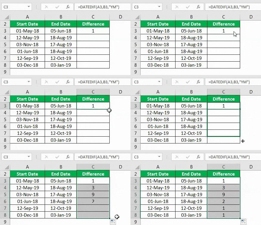
- Step 2: First, we must enter the DATEDIF Formula in the first row and use “YM” as a unit in a formula.
- Step 3: Then, press the “Enter” key, and we will find the days, excluding days and years.
- Step 4: If we drag the formula, we will get the result for all the dates. So, Please find the same in the figure shown below.
Example #6 – Find the years.
- Step 1: Suppose we use the following data to find the years between the two dates.
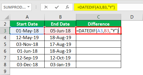
- Step 2: We must enter the DATEDIF formula in the first row first and use “Y” as a unit in a formula.
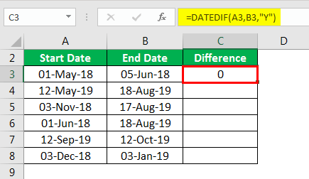
- Step 3: Next, we need to press the “Enter” key, and we will find the years between the two dates.
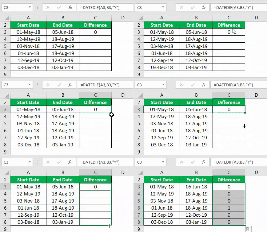
- Step 4: If we drag the formula, we will get the result for all the dates. Therefore, please find the same in the figure shown below.
Advantages
- The DATEDIF function in Excel is easy to use if we want to find the difference between the two dates.
- We can use this formula to see the difference between several days, weeks, or months.
- The DATEDIF function helps us to know the difference between the six parameters.
- The DATEDIF function is so simple. In many cases, we can use it if the unit is a day, year, or month.
- The user needs this function only when it requires more control.
Disadvantages
- The DATEDIF formula in Excel supports only six types of intervals or can help find the difference between only six types of units.
- It cannot control so many types of units like the first day of the week.
- Sometimes this function leads to complexity if we only want to find the difference between days, months, or years.
- Sometimes it may lead to confusion because of many parameters used in one formula.
- The DATEDIF formula in Excel only gives you the formula if you use the correct date format in excelThe date format in Excel can be changed either from the “number format” of the Home tab or the “format cells” option of the context menu.read more.
Things to Remember
- For the DATEDIF formula in Excel to figure months accurately, the end date should be greater than the start date; otherwise, the formula may give the #NUM error.
- The outcomes returned by DATEDIF and YEAR/MONTH formulas are not constantly indistinguishable because they work dependent on various standards. For example, the Excel DATEDIF work restores the number of whole calendar months between the dates, while the YEAR/MONTH equation works on months’ numbers.
- We must always select the correct unit in a formula.
- Excel cannot help us give instructions to fill the DATEDIF formula like other functions.
- It is also recommended not to use “MD” as units because sometimes it gives a negative value.
- Always make sure to use data format while calculating the difference between the values.
- The DATEDIF formula in Excel is also useful while calculating the age.
- When Excel does not recognize the date given, it results in the #Value! Error because Excel cannot understand the data argument.
Recommended Articles
This article has been a guide to DATEDIF in Excel. We discuss using the DATEDIF function and Excel examples, and downloadable Excel templates here. You may also look at these useful functions in Excel: –
- VBA Date Function
- Excel Insert Date
- Concatenate Date in Excel
- Today’s Date in Excel
Reader Interactions









![Format Cells dialog, Custom command, [h]:mm type](https://support.content.office.net/en-us/media/2edbd461-d4c5-49a7-a5a2-b6d9329c0411.png)
