What is a dropdown list?
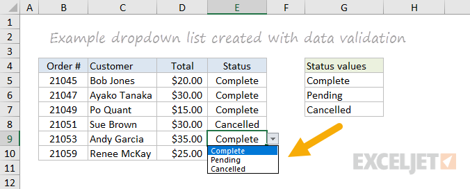
Dropdown lists allow users to select a value from a predefined list. This makes it easy for users to enter only data that meets requirements. Dropdown lists are implemented as a special kind of data validation. The screen below shows a simple example. In column E, the choices are Complete, Pending, or Cancelled, and these values are pulled automatically from the range G5:G7:
Dropdown lists are easy to create and use. But once you start to use dropdown menus in your spreadsheets, you’ll inevitably run into a challenge: how can you make the values in one dropdown list depend on the values in another? In other words, how can you make a dropdown list dynamic?
Here are some examples:
- a list of cities that depends on the selected country
- a list of flavors that depends on type of ice cream
- a list of models that depends on manufacturer
- a list of foods that depends on category
These kind of lists are called dependent dropdowns, since the list depends on another value. They are created with data validation, using a custom formula based on the INDIRECT function and named ranges. This may sound complicated, but it is actually very simple, and a great example of how INDIRECT can be used.
Read on to see how to create dependent dropdown lists in Excel.
Dependent dropdown example
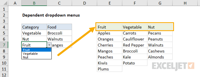
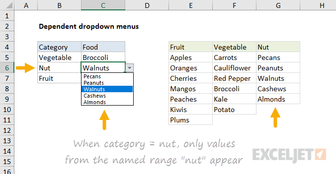
In the example shown below, column B provides a dropdown menu for food Category, and column C provides options in the chosen category. If the user selects «Fruit», they see a list of fruits, if they select «Nut», they see a list of nuts, and if they select «Vegetable», they see a list of vegetables.
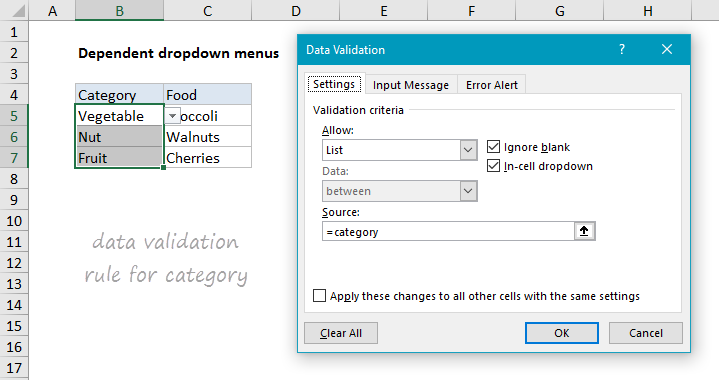
The data validation in column B uses this custom formula:
=category
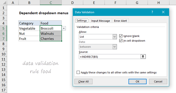
And the data validation in column C uses this custom formula:
=INDIRECT(B5)
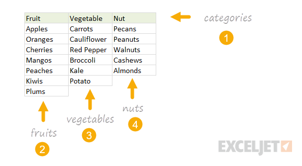
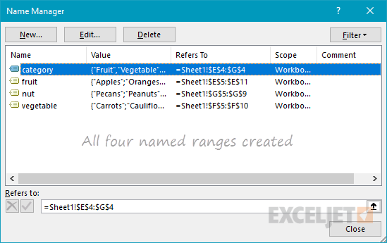
Where the worksheet contains the following named ranges:
category = E4:G4
vegetable = F5:F10
nut = G5:G9
fruit = E5:E11
How this works
The key to this technique is named ranges + the INDIRECT function. INDIRECT accepts text values and tries to evaluate them as cell references. For example, INDIRECT will take the text «A1» and turn it into an actual reference:
=INDIRECT("A1")
=A1
Similarly, INDIRECT will convert the text «A1:A10» into the range A1:A10 inside another function:
=SUM(INDIRECT("A1:A10")
=SUM(A1:A10)
At first glance, you might find this construction annoying, or even pointless. Why complicate a nice simple formula with INDIRECT?
Rest assured, there is a method to the madness 
The beauty of INDIRECT is that it lets you use text exactly like a cell reference. This provides two key benefits:
- You can assemble a text reference inside a formula, which is handy for certain kinds of dynamic references.
- You can pick up text values on a worksheet, and use them like a cell reference in a formula.
In the example on this page, we’re combining the latter idea with named ranges to build dependent dropdown lists. INDIRECT maps text to a named range, which is then resolved to a valid reference. So, in this example, we’re picking up the text values in column B, and using INDIRECT to convert them to cell references by matching existing named ranges, like this:
=INDIRECT(B6)
=INDIRECT("nut")
=G5:G9
B6 resolves to the text «nut» which resolves to the range G5:G9.
How to set up dependent dropdown lists
This section describes how to set up the dependent dropdown lists shown in the example.
1. Create the lists you need. In the example, create a list of fruits, nuts, and vegetables in a worksheet.
2. Create named ranges for each list: category = E4:G4, vegetable = F5:F10, nut = G5:G9, and fruit = E5:E11.
Important: the column headings in E4, F4, and G4 must match the last three named ranges above («vegetable», «nut», and «fruit»). In other words, you must make sure that the named ranges you created match the values in the Category dropdown list.
3. Create and test a data validation rule to provide a dropdown list for Category using the following custom formula:
=category
Note: just to be clear, the named range «category» is used for readability and convenience only – using a named range here is not required. Also note data validation with a list works fine with both horizontal and vertical ranges – both will be presented as a vertical dropdown menu.
4. Create a data validation rule for the dependent dropdown list with a custom formula based on the INDIRECT function:
=INDIRECT(B5)
In this formula, INDIRECT simply evaluates values in column B as references, which links them to the named ranges previously defined.
5. Test the dropdown lists to make sure they dynamically respond to values in column B.
Note: the approach we are taking here is not case-sensitive. The named range is called «nut» and the value in B6 is «Nut» but the INDIRECT function correctly resolves to the named range, even though case differs.
Dealing with spaces
Named ranges don’t allow spaces, so the usual convention is to use underscore characters instead. So, for example, if you want to create a named range for ice cream, you would use ice_cream. This works fine, but dependent dropdown lists will break if they try to map «ice cream» to «ice_cream». To fix this problem you can use a more robust custom formula for data validation:
=INDIRECT(SUBSTITUTE(A1," ","_"))
This formula still uses INDIRECT to link the text value in A1 to a named range, but before INDIRECT runs, the SUBSTITUTE function replaces all spaces with underscores. If the text contains no spaces, SUBSTITUTE has no effect.
Practice file
The example file is attached below – check it out to see how it works. If you want to learn the technique yourself, I’d recommend you build a file of your own. The best way to learn is by doing.
This example describes how to create dependent drop-down lists in Excel. Here’s what we are trying to achieve:
The user selects Pizza from a drop-down list.
As a result, a second drop-down list contains the Pizza items.
To create these dependent drop-down lists, execute the following steps.
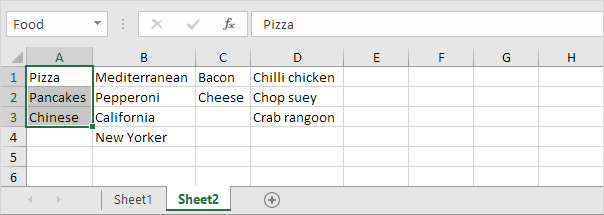
1. On the second sheet, create the following named ranges.
| Name | Range Address |
|---|---|
| Food | A1:A3 |
| Pizza | B1:B4 |
| Pancakes | C1:C2 |
| Chinese | D1:D3 |
2. On the first sheet, select cell B1.
3. On the Data tab, in the Data Tools group, click Data Validation.
The ‘Data Validation’ dialog box appears.
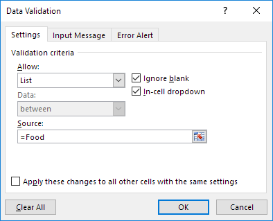
4. In the Allow box, click List.
5. Click in the Source box and type =Food.
6. Click OK.
Result:
7. Next, select cell E1.
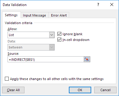
8. In the Allow box, click List.
9. Click in the Source box and type =INDIRECT($B$1).
10. Click OK.
Result:
Explanation: the INDIRECT function returns the reference specified by a text string. For example, the user selects Chinese from the first drop-down list. =INDIRECT($B$1) returns the Chinese reference. As a result, the second drop-down lists contains the Chinese items.
We begin with a table of Divisions where each Division contains a list of Apps.
The goal is to have the user select from the first drop down list a Division name. Next, the user will select an App from the second drop down list. The key is to only display the apps associated with the selected Division from the first drop down list.
NOTE: In the real world, the list of Divisions and Apps would likely be placed on a separate (possible hidden) sheet, or the list would be placed somewhere far away from the data entry portion of the sheet where the user is not likely to ever find. For this example, we are placing the list close to the user-area to make the demonstration easier to follow.
Creating the First Drop Down List (Division)
The first drop down list will allow the user to select a Division. This one is simple.
We begin by creating a Data Validation drop down list for cell A5 that points to the Divisions listed in cells F4 through H4.
- Select cell A5
- Select Data (tab) -> Data Tools (group) -> Data Validation
- In the Data Validation dialog box, set Allow to “List” and Source to “=$F$4:$H$4”
- Click OK
To get the drop down list to appear for multiple rows, select A5 and copy/paste the contents to adjacent cells (ex: A6:A20).
Creating the Second Drop Down List (App)
As stated earlier, we want the second list of Apps to only show items based on the selected Division from the first drop down list.
Using the OFFSET function
We will use the OFFSET function to select Apps from one of the three listed Divisions.
If you’re not familiar with the OFFSET function, it allows us to start from a defined point then moves away from that point by a set number of rows and/or columns. This establishes a new start point. From here, we can select a set number of rows and/or columns.
The OFFSET function has the following syntax:
OFFSET(reference, rows, cols, [height], [width])
- reference – the cell or range of cells you want to base the offset (e. the starting point).
- rows – the number of rows down or up you want to move. A positive number moves down; a negative number moves up.
- cols – the number of columns right or left you want to move. A positive number moves right; a negative number moves left.
- [height] – the number of rows you want returned. This must be a positive number.
- [width] – the number of columns you want returned. This must be a positive number.
NOTE: For an explanation of the OFFSET function, see this post/video.
Ultimately, we need to create this formula in the Data Validation dialog box.
Since the Data Validation dialog box does not possess the IntelliSense feature that is so helpful when writing formulas, we will write and test our formula in a standard Excel cell.
Once we have the formula working, we will transfer it to the Data Validation tool for its final test.
Establishing the Starting Point
We will always begin our search for Apps from the upper-left corner of our table (cell F4).
Start the OFFSET function as follows.
=OFFSET($F$4We need to make this reference to cell A4 as an absolute reference so each copied/pasted version begins from the same point.
Moving Down or Up
Next, we tell OFFSET how many rows to move down or up. The Apps list begins 1 row below our start point, so we assign a value of 1 to the rows argument.
=OFFSET($F$4, 1Moving Right or Left
Now we tell OFFSET how many columns to move right or left.
This is determined by the user’s Division selection from the first drop down list.
For this, we can use the MATCH function to locate the selected Division in cell A5 from the list of Division in cells F4 through H4. We also need to match exactly (0 in the last argument).
=OFFSET($F$4, 1, MATCH($A5, $F$4:$H$4, 0)NOTE: We only “locked” the “A” part of the “A5” reference because we don’t want to point to other columns when we replicate this to adjacent cells, but we do want to point to other rows when creating additional drop downs. If that’s a bit unclear, stick with us because it will become clearer very soon.
If we highlight the MATCH portion of the formula and press F9, we can see MATCH returns a number indicating the discovered position in the search range.
NOTE: Remember to press CTRL-Z to undo your formula back to its original structure.
The Problem with MATCH
A minor issue we have with MATCH is that it counts cells beginning with the value 1.
This means that “Productivity” is in the first column of the data, “Game” is in the second column, and “Utility” is in the third column.
Because we’re trying to inform OFFSET how many columns to move to the right, these values are incorrect.
If we want “Productivity”, we don’t want to move left or right. If we want “Game”, we want to move 1 column to the right, and if we want “Utility”, we want to move 2 columns to the right.
We need to reduce the returned value of MATCH by 1 to adjust for this discrepancy.
=OFFSET($F$4, 1, MATCH($A5, $F$4:$H$4, 0) – 1Selecting the Height to Return
We dropped 1 row from the start point to land on the first App. We also moved right to the proper Division column.
The tricky part is to determine the number of rows to select. This will be the list of Apps that will drives the second drop down list.
Notice that our three lists do not contain the same number of items.
Temporarily, we will treat each list as if they contained 15 items. This will allow us to see if the [height] argument is working. Later, we’ll make the height selection dynamic so it will return the perfect number of Apps for our second drop down list.
=OFFSET($F$4, 1, MATCH($A5, $F$4:$H$4, 0) – 1, 15For any columns that contain less than 15 Apps, this will produce empty slots in the Data Validation drop down list. If you’re okay with that, you can leave the [height] argument set to the largest expected list length. This could be a problem if one list has hundreds of items while another list has only dozens.
Like I said a moment ago, we’ll start statically then make it dynamic later, so we eliminate the empty slots.
Selecting the Width to Return
We only ever want a single column of Apps to be returned by the OFFSET function, so we will set the [width] argument to 1.
=OFFSET($F$4, 1, MATCH($A5, $F$4:$H$4, 0) – 1, 15, 1)Setting Up Data Validation
Now that we have completed our test formula, it’s time to use the logic in a Data Validation drop down list.
- Select cell B5
- Highlight the OFFSET/MATCH formula displayed in the Formula Bar
- Copy the formula to memory
- Press ESC to get out of Edit Mode
- Select Data (tab) -> Data Tools (group) -> Data Validation
- In the Data Validation dialog box, set Allow to “List”
- In the Source field, paste the recently copied OFFSET/MATCH formula
- Click OK
Testing the OFFSET/MATCH Formula
If we select a Division from the first drop down list (A5), we then see the list of related Apps in the second drop down list (B5).
Because we are using a fixed [height] argument, we see blank slots for any Division where the Apps list is less than 15.
Getting the Perfect Height
To get a list of Apps that do not display blank slots at the bottom, we need to calculate the height of the selected Division’s Apps.
We need to take the previously hard-coded “15” for the [height] argument and make it dynamic.
Enter the COUNTA Function
A perfect way to determine the number of Apps in a give Division is to use the COUNTA function.
As a test, we select an unused cell in our sheet and write the following formula:
=COUNTA(F5:F19)This yields a result of 15.
If we point the COUNTA function to G5:G19, we get 12, and if we point the COUNTA function to H5:H19, we get 13.
We don’t want to hard-code the count range, we want the range to be based on the selected Division.
We can replace the hard-coded range with the same OFFSET formula used earlier.
=COUNTA(OFFSET($F$4, 1, MATCH($A5, $F$4:$H$4, 0) – 1, 15, 1)NOTE: the “15” defined in the [height] argument represents the largest number of Apps we would expect to see in any given Division. You should set this value to whatever number you believe you would never reach, such as =COUNTA(OFFSET($F$4, 1, MATCH($A5, $F$4:$H$4, 0) – 1, 500, 1).
Testing the COUNTA Formula
In cell A5, if we select “Productivity” we are returned a value of 15. If we select “Game” we are returned a value of 12, and if we select “Utility” we are returned a value of 13.
Updating the Data Validation Formula
Our final step is to update the formula previously placed in the Data Validation tool for cell B5 to include this dynamic logic for [height] calculations.
- Select the cell that contains the temporary COUNTA formula
- Highlight the COUNTA/OFFSET formula displayed in the Formula Bar
- Copy the formula to memory
- Press ESC to get out of Edit Mode
- Select cell B5
- Select Data (tab) -> Data Tools (group) -> Data Validation
- In the Source field, remove the “15” from the original formula and paste the recently copied COUNTA/OFFSET formula
- Click OK
=OFFSET($F$4, 1, MATCH($A5, $F$4:$H$4, 0) – 1, COUNTA(OFFSET($F$4, 1, MATCH($A5, $F$4:$H$4, 0) – 1, 15, 1)), 1)Testing the Updated Formula
If we select a Division form cell A5 that has less than 15 Apps, we are no longer presented with empty slots at the bottom of the Apps drop down list (B5).
Copying the Data Validation to Adjacent Cells
To replicate the second Data Validation drop down list to the row cells below cell B5:
- Select cell B5
- Press Copy
- Select your destination cells (ex: B6:B15)
- Right-click the highlighted range and select “Paste Special…”
- In the Paste Special dialog box, select Validation and click OK
Final Test
You are now able to select a cell from the “Select Division” column, select a Division, then click the corresponding “Select App” cell to be presented with the Apps for the selected Division.
Granted, I did say that we would use a single formula. I never said it would be short and simple.
The nice thing is that with a small bit of practice, this formula is fairly easy to write. You could even copy/paste it form project to project, reusing it with just minor modifications.
I think it’s easier to stick to a single strategy for building these dependent drop down lists and get good at it, versus learning dozens of other techniques.
Yes, some of those other techniques may be more efficient or have more features, but unless you need fancy and exotic, this one will do just fine.
Practice Workbook
Feel free to Download the Workbook HERE.
Published on: March 26, 2020
Last modified: February 26, 2023
Leila Gharani
I’m a 5x Microsoft MVP with over 15 years of experience implementing and professionals on Management Information Systems of different sizes and nature.
My background is Masters in Economics, Economist, Consultant, Oracle HFM Accounting Systems Expert, SAP BW Project Manager. My passion is teaching, experimenting and sharing. I am also addicted to learning and enjoy taking online courses on a variety of topics.
Dependent Drop Down Lists allows you to validate the data and make the data entry and data filtering very smooth and time-saving. Dependent Drop Down Lists make chances of fewer errors in one’s worksheet. The prerequisites for learning Dependent Drop Down List is Create from Selection and Drop Down List.
Create From Selection
Create from selection helps you to create a named range of a cell. For Example, the Data set is Web Development, Data Structures and Data Analytics, and the skills required to master them.
Steps to Create Drop-Down Lists
Step 1: Go to the Formulas tab, you will find an option Clear from Selection.
Step 2: Select the column, you want to create a named range, here E6:E11.
Step 3: Click on the Create From Selection and a pop up appears.
Step 4: This pop up tells from which value you want to create a named range. More generally we will be using the Top row. The top row specifies that the name of the selected range will be the value written in the Top row. Click ok and a named range is obtained from E6:E11.
Step 5: Click on the Name box and you will find Web Development added to the Name box list.
Step 6: By clicking on the Web development in the Name box, you will be directed to E7:E9. With this, you could be redirected back to the name range despite you being anywhere in your worksheet.
Step 7: Similarly, create a named range for Data Structures and Data Analytics also.
Step 8: Currently, you might not be able to understand the benefit of Create from Selection but as soon as you will study Dependent Dropdown List in Excel, you will understand the power of Create from Selection.
Note: The Scope of Create with Selection is in a work book and not in an individual Worksheet. i.e. if you create multiple worksheets then also the list inside the Name Box will retain itself.
Drop Down List in Excel
Drop Down List in Excel helps to limit the data that you want to enter in your worksheet. For Example, A list of Students is given and we want to enter the data whether that particular student is Pass or Fail. This task can be achieved with help of Drop Down List in Excel.
Steps to Create
Step 1: Select the cells in which you want to apply Data Validation.
Step 2. Go to Data Tab, and click on the Data Validation.
Step 3: Three options appear, again click on Data Validation.
Step 4: A pop-up opens. Inside the Allow, select the type of data you want to allow in that Drop Down List. Most frequently, we use List. So, click on List.
Step 5: A Source Option appears. Now there can be two ways to fill the Source Option either write the Text that you want to allow inside that cell or select the cells inside the worksheet whose value you want to allow in your List. After that click Ok.
Step 6: Now the List looks like this. You could select any value from that list.
Step 7: This makes our work easier and faster.
Dependent Drop Down List in Excel
Now you know about Create From Selection and Drop Down List in Excel. Dependent Drop Down List is the advanced version of Drop Down List. In this, we have Dependencies of Dependencies. We could Create as many dependencies as we want.
Consider a data set with Name and Age.
Steps to Create
Step 1: Select the whole Data Set and go to the Formula tab and click on Create From Selection.
Step 2: A pop-up appears select Top-Row only. Click Ok.
Step 3: In the Name Box you have got Name and Age.
Step 4: Try going to any cell on which you want to apply Data Validation. For example E14. Then Go to Data Tab and click Data Validation. A pop-up appears.
Step 5: Select List in the Allow section.
Step 6: Select the Cells in which you want to have Data Validation. Click Ok. Your Drop Down List is Created.
Step 7: Select any other cell in which you want to apply the Dependent Drop Down List. For example E15. Again Go to Data Tab and click on Data validation and a pop-up appears.
Step 8: Select List in the Allow Section and Use =INDIRECT(REF_SRC) function in the source as shown in the image. For Example, =INDIRECT(E14). and click Ok.
INDIRECT function returns a valid cell reference from a given text String.
Step 9: Hence, you have Created the Dependent Drop Down List which changes with the Drop Down List.

